
Uncertainty Quantification in CO2 Trapping Mechanisms: A Case Study of PUNQ-S3 Reservoir Model Using Representative Geological Realizations and Unsupervised Machine Learning

Abstract
:1. Introduction
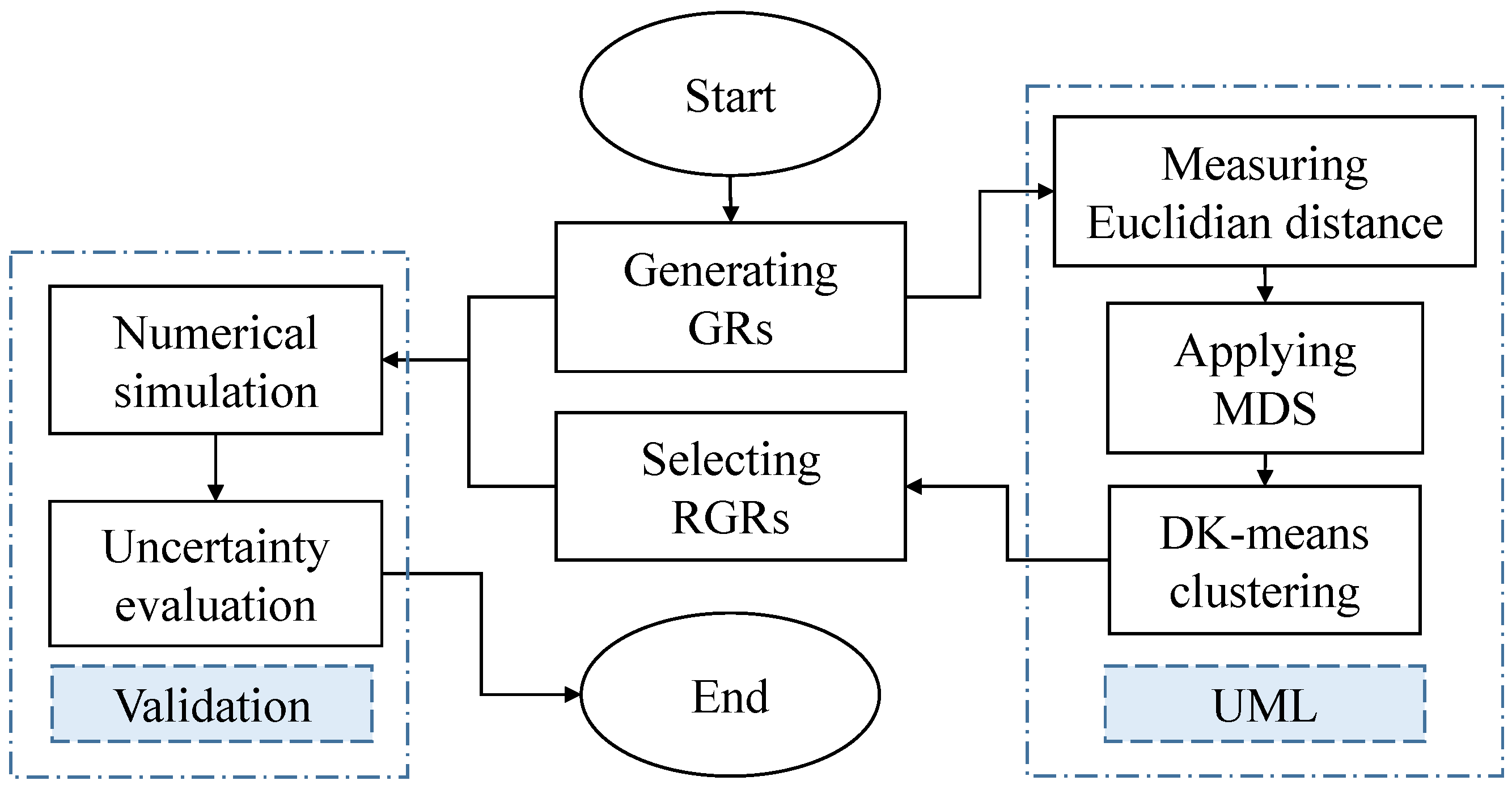
2. Methodology
2.1. Generate Multiple Geological Realizations (GRs)
2.2. Euclidean Distance Measurement between Realizations
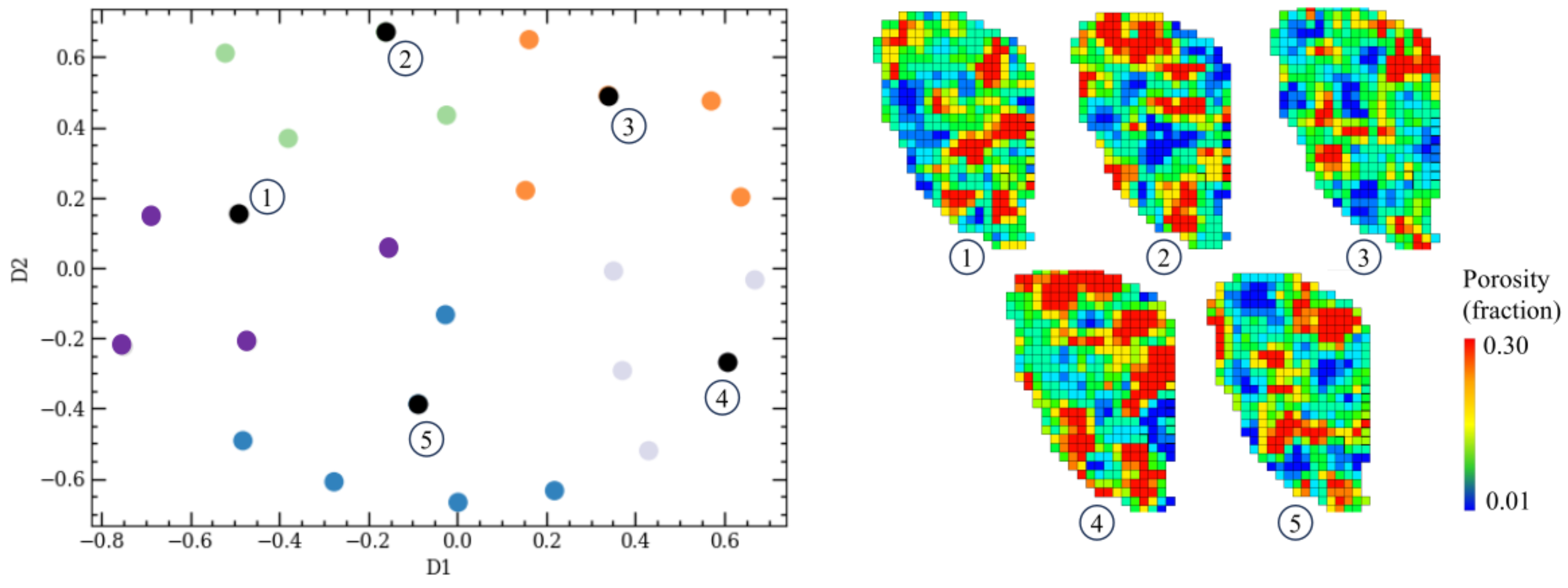
2.3. Multidimensional Scaling (MDS)
2.4. Deterministic K-Means (DK-Means) Clustering
2.5. Numerical Simulation and Uncertainty Evaluation
3. Model Description
3.1. Geometric Model
3.2. Well Control Configurations
3.3. Reference Simulation Outputs
4. Results
5. Conclusions
Author Contributions
Funding
Data Availability Statement
Conflicts of Interest
Abbreviations
| BHP | Bottom Hole Pressure |
| CCS | Carbon Capture and Storage |
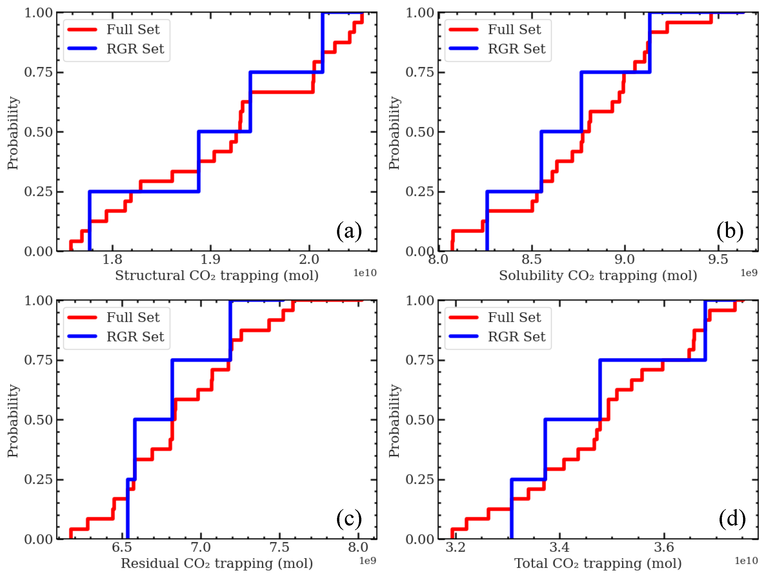
| CDF | Cumulative Distribution Function |
| CMG-GEM | Canada Modeling Group-Generalized Equation of State Model |
| DK-means | Deterministic K-means |
| GR | Geological Realization |
| GTT | Generalized Travel Time |
| IP | Injection Plan |
| KS | Kolmogorov–Smirnov |
| LHS | Latin Hypercube Sampling |
| MDS | Multidimensional Scaling |
| RGR | Representative Geological Realization |
| RQI | Reservoir Quality Index |
| STG | Surface Gas Rate |
| UML | Unsupervised Machine Learning |
References
- Tadjer, A.; Bratvold, R.B. Managing Uncertainty in Geological CO2 Storage Using Bayesian Evidential Learning. Energies 2021, 14, 1557. [Google Scholar] [CrossRef]
- Wilkinson, M.; Polson, D. Uncertainty in regional estimates of capacity for carbon capture and storage. Solid Earth 2019, 10, 1707–1715. [Google Scholar] [CrossRef]
- Harp, D.R.; Stauffer, P.H.; O’Malley, D.; Jiao, Z.; Egenolf, E.P.; Miller, T.A.; Martinez, D.; Hunter, K.A.; Middleton, R.S.; Bielicki, J.M.; et al. Development of robust pressure management strategies for geologic CO2 sequestration. Int. J. Greenh. Gas Control 2017, 64, 43–59. [Google Scholar] [CrossRef]
- Jin, L.; Hawthorne, S.; Sorensen, J.; Pekot, L.; Kurz, B.; Smith, S.; Heebink, L.; Herdegen, V.; Bosshart, N.; Torres, J.; et al. Advancing CO2 enhanced oil recovery and storage in unconventional oil play—Experimental studies on Bakken shales. Appl. Energy 2017, 208, 171–183. [Google Scholar] [CrossRef]
- Nilsen, H.M.; Lie, K.A.; Andersen, O. Analysis of CO2 trapping capacities and long-term migration for geological formations in the Norwegian North Sea using MRST-co2lab. Comput. Geosci. 2015, 79, 15–26. [Google Scholar] [CrossRef]
- Diao, Y.; Zhu, G.; Li, X.; Bai, B.; Li, J.; Wang, Y.; Zhao, X.; Zhang, B. Characterizing CO2 plume migration in multi-layer reservoirs with strong heterogeneity and low permeability using time-lapse 2D VSP technology and numerical simulation. Int. J. Greenh. Gas Control. 2020, 92, 102880. [Google Scholar] [CrossRef]
- Langhi, L.; Strand, J.; Ricard, L. Flow modelling to quantify structural control on CO2 migration and containment, CCS South West Hub, Australia. Pet. Geosci. 2021, 27, petgeo2020-094. [Google Scholar] [CrossRef]
- Shepherd, A.; Martin, M.; Hastings, A. Uncertainty of modelled bioenergy with carbon capture and storage due to variability of input data. GCB Bioenergy 2021, 13, 691–707. [Google Scholar] [CrossRef]
- Jia, W.; McPherson, B.; Pan, F.; Dai, Z.; Xiao, T. Uncertainty quantification of CO2 storage using Bayesian model averaging and polynomial chaos expansion. Int. J. Greenh. Gas Control 2018, 71, 104–115. [Google Scholar] [CrossRef]
- Sun, W.; Durlofsky, L.J. Data-space approaches for uncertainty quantification of CO2 plume location in geological carbon storage. Adv. Water Resour. 2019, 123, 234–255. [Google Scholar] [CrossRef]
- Mahjour, S.K.; Faroughi, S.A. Risks and uncertainties in carbon capture, transport, and storage projects: A comprehensive review. Gas Sci. Eng. 2023, 119, 205117. [Google Scholar] [CrossRef]
- Bueno, J.F.; Drummond, R.D.; Vidal, A.C.; Sancevero, S.S. Constraining uncertainty in volumetric estimation: A case study from Namorado Field, Brazil. J. Pet. Sci. Eng. 2011, 77, 200–208. [Google Scholar] [CrossRef]
- Mahjour, S.K.; Santos, A.A.S.; Correia, M.G.; Schiozer, D.J. Scenario reduction methodologies under uncertainties for reservoir development purposes: Distance-based clustering and metaheuristic algorithm. J. Pet. Explor. Prod. Technol. 2021, 11, 3079–3102. [Google Scholar] [CrossRef]
- Schiozer, D.J.; dos Santos, A.A.d.S.; de Graça Santos, S.M.; von Hohendorff Filho, J.C. Model-based decision analysis applied to petroleum field development and management. Oil Gas Sci. Technol. Rev. D’Ifp Energies Nouv. 2019, 74, 46. [Google Scholar] [CrossRef]
- Trehan, S.; Carlberg, K.T.; Durlofsky, L.J. Error modeling for surrogates of dynamical systems using machine learning. Int. J. Numer. Methods Eng. 2017, 112, 1801–1827. [Google Scholar] [CrossRef]
- Mahjour, S.K.; da Silva, L.O.M.; Meira, L.A.A.; Coelho, G.P.; dos Santos, A.A.d.S.; Schiozer, D.J. Evaluation of unsupervised machine learning frameworks to select representative geological realizations for uncertainty quantification. J. Pet. Sci. Eng. 2022, 209, 109822. [Google Scholar] [CrossRef]
- Faroughi, S.A.; Soltanmohammadi, R.; Datta, P.; Mahjour, S.K.; Faroughi, S. Physics-informed neural networks with periodic activation functions for solute transport in heterogeneous porous media. Mathematics 2023, 12, 63. [Google Scholar] [CrossRef]
- Faroughi, S.A.; Pawar, N.M.; Fernandes, C.; Raissi, M.; Das, S.; Kalantari, N.K.; Mahjour, S.K. Physics-Guided, Physics-Informed, and Physics-Encoded Neural Networks and Operators in Scientific Computing: Fluid and Solid Mechanics. J. Comput. Inf. Sci. Eng. 2024, 24, 040802. [Google Scholar] [CrossRef]
- Datta, P.; Faroughi, S.A. A multihead LSTM technique for prognostic prediction of soil moisture. Geoderma 2023, 433, 116452. [Google Scholar] [CrossRef]
- Vaziri, P.; Sedaee, B. A machine learning-based approach to the multiobjective optimization of CO2 injection and water production during CCS in a saline aquifer based on field data. Energy Sci. Eng. 2023, 11, 1671–1687. [Google Scholar] [CrossRef]
- Shirangi, M.G.; Durlofsky, L.J. A general method to select representative models for decision making and optimization under uncertainty. Comput. Geosci. 2016, 96, 109–123. [Google Scholar] [CrossRef]
- Lee, K.; Jung, S.; Lee, T.; Choe, J. Use of clustered covariance and selective measurement data in ensemble smoother for three-dimensional reservoir characterization. J. Energy Resour. Technol. 2017, 139. [Google Scholar] [CrossRef]
- Mahjour, S.K.; Correia, M.G.; Santos, A.A.d.S.d.; Schiozer, D.J. Using an integrated multidimensional scaling and clustering method to reduce the number of scenarios based on flow-unit models under geological uncertainties. J. Energy Resour. Technol. 2020, 142, 063005. [Google Scholar] [CrossRef]
- Haddadpour, H.; Niri, M.E. Uncertainty assessment in reservoir performance prediction using a two-stage clustering approach: Proof of concept and field application. J. Pet. Sci. Eng. 2021, 204, 108765. [Google Scholar] [CrossRef]
- Hinton, G.; Sejnowski, T.J. Unsupervised Learning: Foundations of Neural Computation; MIT Press: Cambridge, MA, USA, 1999. [Google Scholar] [CrossRef]
- Liu, Z.; Forouzanfar, F. Ensemble clustering for efficient robust optimization of naturally fractured reservoirs. Comput. Geosci. 2018, 22, 283–296. [Google Scholar] [CrossRef]
- Lee, K.; Jung, S.; Choe, J. Ensemble smoother with clustered covariance for 3D channelized reservoirs with geological uncertainty. J. Pet. Sci. Eng. 2016, 145, 423–435. [Google Scholar] [CrossRef]
- Park, J.; Jin, J.; Choe, J. Uncertainty quantification using streamline based inversion and distance based clustering. J. Energy Resour. Technol. 2016, 138, 012906. [Google Scholar] [CrossRef]
- Pinheiro, M.; Emery, X.; Miranda, T.; Lamas, L.; Espada, M. Modelling geotechnical heterogeneities using geostatistical simulation and finite differences analysis. Minerals 2018, 8, 52. [Google Scholar] [CrossRef]
- Mahjour, S.K.; Faroughi, S.A. Selecting representative geological realizations to model subsurface CO2 storage under uncertainty. Int. J. Greenh. Gas Control. 2023, 127, 103920. [Google Scholar] [CrossRef]
- Juanes, R.; Spiteri, E.; Orr Jr, F.; Blunt, M. Impact of relative permeability hysteresis on geological CO2 storage. Water Resour. Res. 2006, 42, 2005WR004806. [Google Scholar] [CrossRef]
- Pilger, G.; Costa, J.; Koppe, J. The benefits of Latin Hypercube Sampling in sequential simulation algorithms for geostatistical applications. Appl. Earth Sci. 2008, 117, 160–174. [Google Scholar] [CrossRef]
- Damblin, G.; Couplet, M.; Iooss, B. Numerical studies of space-filling designs: Optimization of Latin Hypercube Samples and subprojection properties. J. Simul. 2013, 7, 276–289. [Google Scholar] [CrossRef]
- Suzuki, S.; Caers, J.K. History matching with an uncertain geological scenario. In Proceedings of the SPE Annual Technical Conference and Exhibition, San Antonio, TX, USA, 24–27 September 2006. [Google Scholar] [CrossRef]
- Scheidt, C.; Caers, J. Representing spatial uncertainty using distances and kernels. Math. Geosci. 2009, 41, 397–419. [Google Scholar] [CrossRef]
- Mahjour, S.K.; Al-Askari, M.K.G.; Masihi, M. Identification of flow units using methods of Testerman statistical zonation, flow zone index, and cluster analysis in Tabnaak gas field. J. Pet. Explor. Prod. Technol. 2016, 6, 577–592. [Google Scholar] [CrossRef]
- Shan, L.; Cao, L.; Guo, B. Identification of flow units using the joint of WT and LSSVM based on FZI in a heterogeneous carbonate reservoir. J. Pet. Sci. Eng. 2018, 161, 219–230. [Google Scholar] [CrossRef]
- Oliveira, G.; Santos, M.; Roque, W. Constrained clustering approaches to identify hydraulic flow units in petroleum reservoirs. J. Pet. Sci. Eng. 2020, 186, 106732. [Google Scholar] [CrossRef]
- Yu, P. Hydraulic unit classification of un-cored intervals/wells and its influence on the productivity performance. J. Pet. Sci. Eng. 2021, 197, 107980. [Google Scholar] [CrossRef]
- Belhouchet, H.; Benzagouta, M.; Dobbi, A.; Alquraishi, A.; Duplay, J. A new empirical model for enhancing well log permeability prediction, using nonlinear regression method: Case study from Hassi-Berkine oil field reservoir–Algeria. J. King Saud Univ. Eng. Sci. 2021, 33, 136–145. [Google Scholar] [CrossRef]
- Faroughi, S.A.; Faroughi, S.; McAdams, J. A prompt sequential method for subsurface flow modeling using the modified multi-scale finite volume and streamline methods. Int. J. Num. Anal. Model. 2013, 4, 129–150. [Google Scholar]
- Bordbar, A.; Faroughi, S.; Faroughi, S.A. A pseudo-TOF based streamline tracing for streamline simulation method in heterogeneous hydrocarbon reservoirs. Am. J. Eng. Res. 2018, 7, 23–31. [Google Scholar]
- Soong, Y.; Crandall, D.; Howard, B.H.; Haljasmaa, I.; Dalton, L.E.; Zhang, L.; Lin, R.; Dilmore, R.M.; Zhang, W.; Shi, F.; et al. Permeability and mineral composition evolution of primary seal and reservoir rocks in geologic carbon storage conditions. Environ. Eng. Sci. 2018, 35, 391–400. [Google Scholar] [CrossRef]
- Xu, R.; Li, R.; Ma, J.; He, D.; Jiang, P. Effect of mineral dissolution/precipitation and CO2 exsolution on CO2 transport in geological carbon storage. Accounts Chem. Res. 2017, 50, 2056–2066. [Google Scholar] [CrossRef]
- George, N.J.; Ekanem, A.M.; Ibanga, J.I.; Udosen, N.I. Hydrodynamic implications of aquifer quality index (AQI) and flow zone indicator (FZI) in groundwater abstraction: A case study of coastal hydro-lithofacies in South-eastern Nigeria. J. Coast. Conserv. 2017, 21, 759–776. [Google Scholar] [CrossRef]
- Ontañón, S. An overview of distance and similarity functions for structured data. Artif. Intell. Rev. 2020, 53, 5309–5351. [Google Scholar] [CrossRef]
- Fouedjio, F. Multidimensional Scaling. In Encyclopedia of Mathematical Geosciences; Springer: Cham, Switzerland, 2023; pp. 938–945. [Google Scholar] [CrossRef]
- Borg, I.; Groenen, P.J. Modern Multidimensional Scaling: Theory and Applications; Springer: New York, NY, USA, 2005. [Google Scholar] [CrossRef]
- Jothi, R.; Mohanty, S.K.; Ojha, A. DK-means: A deterministic k-means clustering algorithm for gene expression analysis. Pattern Anal. Appl. 2019, 22, 649–667. [Google Scholar] [CrossRef]
- Nidheesh, N.; Nazeer, K.A.; Ameer, P. An enhanced deterministic K-Means clustering algorithm for cancer subtype prediction from gene expression data. Comput. Biol. Med. 2017, 91, 213–221. [Google Scholar] [CrossRef] [PubMed]
- Xue, B.; Oldfield, C.J.; Dunker, A.K.; Uversky, V.N. CDF it all: Consensus prediction of intrinsically disordered proteins based on various cumulative distribution functions. FEBS Lett. 2009, 583, 1469–1474. [Google Scholar] [CrossRef] [PubMed]
- Ferreira, C.J.; Davolio, A.; Schiozer, D.J. Evaluation of the Discrete Latin Hypercube with Geostatistical Realizations Sampling for History Matching Under Uncertainties for the Norne Benchmark Case. In Proceedings of the OTC Brasil, Rio de Janeiro, Brazil, 24–26 October 2017. [Google Scholar] [CrossRef]
- Floris, F.J.; Bush, M.; Cuypers, M.; Roggero, F.; Syversveen, A.R. Methods for quantifying the uncertainty of production forecasts: A comparative study. Pet. Geosci. 2001, 7, S87–S96. [Google Scholar] [CrossRef]
- Pan, B.; Liu, K.; Ren, B.; Zhang, M.; Ju, Y.; Gu, J.; Zhang, X.; Clarkson, C.R.; Edlmann, K.; Zhu, W.; et al. Impacts of relative permeability hysteresis, wettability, and injection/withdrawal schemes on underground hydrogen storage in saline aquifers. Fuel 2023, 333, 126516. [Google Scholar] [CrossRef]
- Killough, J. Reservoir simulation with history-dependent saturation functions. Soc. Pet. Eng. J. 1976, 16, 37–48. [Google Scholar] [CrossRef]
- Land, C.S. Calculation of imbibition relative permeability for two-and three-phase flow from rock properties. Soc. Pet. Eng. J. 1968, 8, 149–156. [Google Scholar] [CrossRef]
- Maalim, A.A.; Mahmud, H.B.; Seyyedi, M. Assessing roles of geochemical reactions on CO2 plume, injectivity and residual trapping. Energy Geosci. 2021, 2, 327–336. [Google Scholar] [CrossRef]


Disclaimer/Publisher’s Note: The statements, opinions and data contained in all publications are solely those of the individual author(s) and contributor(s) and not of MDPI and/or the editor(s). MDPI and/or the editor(s) disclaim responsibility for any injury to people or property resulting from any ideas, methods, instructions or products referred to in the content. |
© 2024 by the authors. Licensee MDPI, Basel, Switzerland. This article is an open access article distributed under the terms and conditions of the Creative Commons Attribution (CC BY) license (https://creativecommons.org/licenses/by/4.0/).
Share and Cite
Mahjour, S.K.; Badhan, J.H.; Faroughi, S.A. Uncertainty Quantification in CO2 Trapping Mechanisms: A Case Study of PUNQ-S3 Reservoir Model Using Representative Geological Realizations and Unsupervised Machine Learning. Energies 2024, 17, 1180. https://doi.org/10.3390/en17051180
Mahjour SK, Badhan JH, Faroughi SA. Uncertainty Quantification in CO2 Trapping Mechanisms: A Case Study of PUNQ-S3 Reservoir Model Using Representative Geological Realizations and Unsupervised Machine Learning. Energies. 2024; 17(5):1180. https://doi.org/10.3390/en17051180
Chicago/Turabian StyleMahjour, Seyed Kourosh, Jobayed Hossain Badhan, and Salah A. Faroughi. 2024. "Uncertainty Quantification in CO2 Trapping Mechanisms: A Case Study of PUNQ-S3 Reservoir Model Using Representative Geological Realizations and Unsupervised Machine Learning" Energies 17, no. 5: 1180. https://doi.org/10.3390/en17051180