Multi-Output Regression Algorithm-Based Non-Dominated Sorting Genetic Algorithm II Optimization for L-Shaped Twisted Tape Insertions in Circular Heat Exchange Tubes

Abstract

In this study, an optimization method using various multi-output regression models as model proxies within the NSGA-II framework was applied to determine the geometric parameters (P, W, D) of L-shaped twisted tape inserts for achieving the optimal overall heat transfer performance in a circular heat exchange tube. Herein, 4 multi-output regression models, namely, MOLR, MOSVR, MOGPR, and BPNN, were selected as proxy models and trained on a dataset containing 74 groups of data. The training results indicated that the MOGPR model, balancing high accuracy and low error conditions, exhibited moderate training times among the four algorithms. BPNN showed a comparatively lower comprehensive training effect, obtaining training accuracy close to that of the MOGPR algorithm but with approximately twice the training time. The worst fitting performance was gained with the MOSVR algorithm. Due to its fitting performance, the MOSVR algorithm was excluded from the subsequent NSGA-II model proxy. Through multi-objective optimization with NSGA-II, the optimal structural dimensions for three sets of L-shaped twisted tape inserts were obtained to achieve the best overall heat transfer efficiency within the tube.

1. Introduction

Heat exchangers, widely applied as heat exchange tools across various industries, play a significant role in reducing production costs and minimizing energy consumption for enterprises. Researchers worldwide have conducted diverse studies to enhance the thermal efficiency within heat exchangers. Among these investigations, the passive heat transfer enhancement method involving the insertion of twisted tape inserts within heat exchange tubes has been extensively researched. The incorporation of twisted tape inserts enhances heat transfer by prolonging heat exchange time, inducing fluid disturbance, and disrupting the laminar boundary layer on the tube wall. However, the introduction of twisted tape inserts concurrently increases fluid flow resistance. Consequently, determining the optimal and most efficient structure for twisted tape inserts to balance heat transfer enhancement and flow resistance has emerged as a valuable research topic.

Numerous studies have been conducted on the optimization and design of twisted tape inserts. For example, K. Hata [1] investigated the heat transfer effects of a plain twisted tape at three twist ratios (2.39, 3.39, and 4.45) on a short circular heat exchange tube. The experiments were conducted over a range of inlet fluid mass flow rates from 4022 to 15,140 kg/m² s. The study established empirical relationships between the Nusselt number, friction factor, and the inlet flow velocity and twist ratio, generating relevant empirical formulas based on the experimental results. K. Wongcharee [2] conducted heat transfer experiments in circular tubes using alternate clockwise and counter-clockwise twisted tapes (TAs) and plain twisted tapes (TTs). Three twist ratios (3, 4, and 5) were designed for both types of twisted tapes within the Re number range of 830–1990. The results indicated that the Nusselt number, friction factor, and thermal performance factor values for tubes with TA were higher than those for tubes with TT, with the maximum heat transfer efficiency observed at a twist ratio of 3. Similarly, the study concluded with empirical expressions regarding the Nusselt number, friction factor, and thermal performance factor relationships. S.P. Nalavade [3] utilized a novel thermally nonconductive material to manufacture twisted tapes and compared their heat transfer performance with smooth circular tubes at Reynolds numbers ranging from 7000 to 20,000. The experimental results demonstrated that this material helped restrict the thermal energy storage of the twisted tapes, resulting in higher heat transfer efficiency. M.M.K. Bhuiya [4,5] devised a novel configuration consisting of triple concentric twisted tapes, where three concentric twisted tapes were combined. This innovative structure was investigated for its heat transfer performance across four distinct twist ratios: 1.92, 2.88, 4.81, and 6.79. The experimental results revealed that all three parameters, namely, the Nusselt number, friction factor, and thermal enhancement efficiency, exhibited a positive correlation with increasing twist ratio. Additionally, the research established predictive relationships for the final heat transfer outcomes based on the parameters of the twist ratio (y), Reynolds number (Re), and Prandtl number (Pr). In a separate study, K. Nanan [6] explored the heat transfer effectiveness of perforated helical-twisted tapes (P-HTTs), which were created by perforating conventional helical-twisted tapes (HTTs). This innovative approach aimed to reduce fluid resistance in the heat exchange process. The study systematically investigated the heat transfer performance with variations in the perforation diameter ratio (d/w) and perforation pitch ratio (s/w). Empirical correlations for the Nusselt number, friction coefficient, and thermal performance coefficient were derived, demonstrating a remarkable predictive accuracy within a narrow margin of ±4%, ±6%, and ±3%, respectively. It has been shown that researchers commonly fit empirical formulas to experimental data to establish continuous relationships between input parameters and output parameters. However, these empirical formulas are often derived from linear or polynomial relationships. When the heat transfer process deviates from linear relationships, the accuracy and extensibility of empirical formulas are limited. Therefore, there is a need for more algorithms to fit these heat transfer results.

In statistics, the process of establishing a mapping relationship between input parameters and output parameters is referred to as regression. For heat transfer processes, output parameters typically include important factors, such as the Nusselt number and friction factor, characterizing the heat transfer effectiveness and fluid resistance in the heat exchange system. Thus, a regression analysis of heat transfer processes represents a type of multi-output regression problem. Multi-output regression problems are common in both daily life and engineering applications, prompting extensive theoretical and practical research by numerous scholars in this field.

In the realm of theoretical research and practical applications of multi-output regression algorithms, numerous scholars from both domestic and international backgrounds have contributed invaluable insights and experiences. In 1980, Van der Merwe and Zidek [7] introduced a method known as FICY REG (filtered canonical Y-variate regression) for the analysis of multi-output regression problems. Their research demonstrated that this approach outperforms the traditional LS (least squares) method in terms of performance. Xu, Shou [8], and their colleagues developed a multi-output regression machine based on least squares support vector regression, achieving commendable experimental results in the field of pattern recognition. Brudnak [9] proposed a vector-valued version of adaptive support vector regression, offering a novel approach to multi-output regression. Additionally, several other papers have enriched the theoretical foundations and practical algorithms in this field. For instance, Liu et al. [10] introduced the concept of local linear transformation, which transforms the output space of multi-output regression problems from Euclidean space to Riemannian geometric space, achieving notable results in support vector machine regression. Borchani [11] and his team conducted extensive research on multi-output regression, systematically elucidating the advancements and implementation methods in this domain. Focusing on the applications of multi-output regression algorithms across various domains, Xu [12] and colleagues summarized recent research in this area. D. Kocev et al. [13] applied single-objective and multi-objective regression trees with ensemble methods in vegetation studies. They established a comprehensive indicator model for vegetation conditions, enabling the prediction and assessment of vegetation status. E.S. De Lima [14] utilized multi-output regression algorithms in the field of game behavior research to model player behavior and personality, providing support for the implementation of interactive storylines in games. Lopez-Martin [15] employed deep convolutional neural networks in the field of fluid dynamics to construct a short-term fluid dynamics estimator for free models, demonstrating the potential of multi-output regression in the 3D modeling of fluid dynamics. The extensive application of multi-output regression algorithms was demonstrated across various domains in these studies.

In the application of multi-output regression problems in the field of heat transfer, researchers frequently employ machine learning algorithms to fit heat transfer outcomes. Shashwat Bhattacharya [16] constructed multi-output regression models and neural network models to predict Reynolds numbers and Nusselt numbers for turbulent convective heat transfer. These predictive models were compared with the predictions of the Grossmann–Lohse early convection models. The results revealed that while all models provided close predictions, the machine learning model developed in this work offered the best match with experimental and numerical results. Muhammed Zafar Ali Khan [17] utilized an artificial neural network model to regress 300 data points collected from 7 sources. The input parameters included the wing–width ratio (w/W), pitch ratio (P/W), attack angle (α), Reynolds number (Re), and tube length (L), while the output parameters consisted of the Nusselt number (Nu), friction factor (f), and thermal performance factor (η). The model achieved the lowest mean absolute error (MAE) with an intermediate layer structure of 5-10-10-10-1. Jyoti Prakash Panda [18] employed three machine learning methods, namely, polynomial regression (PR), random forest (RF), and an artificial neural network (ANN), for regression analysis of the Reynolds numbers (Re), twist ratio (t), percentage of perforation (p), and the number of twisted tapes (n) against the Nusselt numbers and friction factors inside tubes fitted with twisted tape inserts. The results indicated that the ANN model outperformed the other two. Muhammad Saeed [19] conducted a regression analysis of experimental results using four methods: Support Vector Regression (SVR), artificial neural network (ANN), random forest (RF), and decision tree (DT). After obtaining regression models, the RSM and MOGA methods were employed to optimize the structure of a C-type printed circuit heat exchanger. Nevin Celik’s [20] regression analysis involved the application of four well-known methods: support vector regression (SVR), Gaussian process regression (GPR), random forest (RF), and multilayer perceptron network (MLP) (a form of artificial neural network). Multiple linear regression (MLR) was also applied for comparison. Result analyses revealed that the MLR method yielded the highest R² value, followed by the GPR method. Morteza Esfandyari [21] performed a regression analysis of heat transfer results for a double-pipe heat exchanger using two models: artificial neural networks (ANNs) and adaptive neuro-fuzzy inference systems (ANFISs). The input parameters included the heat transfer rate, Nusselt number, and the number of transfer units (NTUs). Following the acquisition of regression models, the PSO method was used for optimization. The results indicated that the combination of ANN and the PSO method slightly outperformed the combination of ANFIS and the PSO method. Furthermore, researchers have applied machine learning models in various other heat transfer domains, such as nano-fluid microchannel heat sinks [22], spherical dimples [23] inside tubes, double-pipe heat exchangers [24], and helical plate [25] heat exchangers.

In the realm of research in these heat transfer enhancement areas, some researchers have chosen to treat the Nusselt number and friction factor as two separate variables, thereby decomposing the multi-output regression problem into two distinct single-output regression problems. This approach offers the advantage of reduced computational complexity and improved calculation speed. However, it may have shortcomings in terms of the regression results, as it overlooks the interrelationship between the Nusselt number and friction factor.

In this study, four multi-output regression methods (multi-output linear regression, multi-output support vector machine regression, multi-output Gaussian process regression, and BP neural networks) were applied to model the relationship between the geometric parameters of an L-shaped twisted tape insert and the two output parameters: Nusselt number and friction factor. Subsequently, after obtaining the optimal regression models, a multi-objective parameter optimization method, NSGA-II, was utilized to obtain the optimal geometric parameters for the twisted tape insert.

2. Numerical Simulation Preparation

2.1. Physical Model

Figure 1 presents a schematic diagram of the L-shaped twisted tape insert structure applied in this study. Both the overall view and the cross-sectional view of the structure are displayed. As observed in the figure, P refers to the linear distance between two consecutive identical points on the tape, which plays a crucial role in influencing the heat transfer performance of the twisted tape. Additionally, the distance from the inner wall of the twisted tape to the center of the circular tube is denoted as D, impacting the size of the twisted tape and its volume proportion within the heat exchange tube, thus affecting heat transfer performance. Another dimension studied as an input parameter was the width of the L-shaped twisted tape, denoted as W. Variations in this dimension influenced the disturbance and vortex generation effects of the twisted tape on the fluid, making it a significant parameter for investigation.

In addition to the input parameters P, D, and W, the figure also highlights other parameters affecting the twisted tape structure. These include the length of the L-shaped twisted tape (L0), set as a fixed value of 3 mm, and the total length of the twisted tape (L), fixed at 600 mm.

A case study was designed to demonstrate the impact of incorporating L-shaped twisted tape inserts on the heat transfer performance of a heat exchange tube under Re = 3750. The simulation software used for this case study, along with detailed parameter settings and validation progress, is presented in another publication by the same authors within the research field [26]. The simulation results can be observed in Figure 2.

From the streamline plot in Figure 2a, it is evident that the addition of L-shaped twisted tape forces fluid disturbance. The flow velocity is decomposed into two components: one along the flow direction and the other rotating around the twisted tape, thereby prolonging heat exchange time and enhancing fluid disturbance. In Figure 2b, along the flow direction, the fluid temperature gradually increases, but the temperature difference across the section decreases. This is attributed to the increased fluid flow resistance and reduced flow velocity. Consequently, designing an optimal structure to minimize flow resistance becomes essential. Figure 2c presents a detailed cross-sectional view of the L-shaped region of the twisted tape, illustrating fluid convergence in this area and significant disturbance, which is favorable for improving heat transfer efficiency.

2.2. Governing Equation

In the present study, a three-dimensional and steady calculation model was employed. The following assumptions were considered: (1) the working flow is both incompressible and constant, (2) the gravitational impact of water is negligible, and (3) the fluid is characterized as a Newtonian fluid. With these assumptions, the governing equations were formulated as follows:

Continuity equation:

$$\frac{\partial u_i}{\partial x_i}=0 (i=1\sim 3)$$

(1)

Momentum equation:

$$\rho u_i\frac{\partial u_j}{\partial x_i}=-\frac{\partial p}{\partial x_i}+\frac{\partial }{\partial x_i}\left(\mu \frac{\partial u_j}{\partial x_i}\right)(i,j=1\sim 3)$$

(2)

Energy equation:

$$\rho C_p{u}_i\frac{\partial T}{\partial x_i}=\frac{\partial }{\partial x_i}\left(k\frac{\partial T}{\partial x_i}\right)(i,j=1,2,3)$$

(3)

The BSL k-ω turbulent model was utilized in this study, acquired as follows:

$$\frac{\partial u_1}{\partial t}+u_j\frac{\partial u_1}{\partial x_j}=-\frac{1}{\rho }\frac{\partial p}{\partial x_i}+\frac{\partial }{\partial x_j}\left(\left(\nu +v_T\right)\frac{\partial u_1}{\partial x_j}\right)$$

(4)

where u = $u_1$, $\nu$ = $u_2$, x = x₁, and y = x₂. The variable $v_T$ presents the eddy viscosity and is calculated by k/ω, as determined by

$$\frac{\partial k}{\partial t}+u_j\frac{\partial k}{\partial x_j}=\frac{\partial }{\partial x_j}\left(\left(\nu +\sigma v_T\right)\frac{\partial k}{\partial x_j}\right)+{\tau }_{nj}\frac{\partial u_n}{\partial x_j}-{\beta }^{*}k\omega$$

(5)

$$\frac{\partial \omega }{\partial t}+u_j\frac{\partial \omega }{\partial x_j}=\frac{\partial }{\partial x_j}\left(\left(\nu +\sigma v_T\right)\frac{\partial \omega }{\partial x_j}\right)-{\beta }_1{\omega }^2+\lambda \frac{\omega }{k}{\tau }_{nj}\frac{\partial u_n}{\partial x_j}+2\left(1-F_1\right)\frac{\sigma }{\omega }\frac{\partial k}{\partial x_j}\frac{\partial \omega }{\partial x_j}$$

(6)

where $\omega$ denotes the specific dissipation rate, $k$ signifies the turbulent kinetic energy, and $\tau$ represents the residual stress tensor.

The associated constants are ${\beta }_1$ = 0.075, $\sigma$ = 0.5, ${\beta }^{*}$ = 0.09, and $\lambda$ = 0.556. The value of $F_1$ is detailed in [27].

The entirety of heat transfer occurring between the channel wall and water is encompassed by:

$${\dot{Q}}_{air}=\dot{m}{C}_{p,\mathrm{w}\mathrm{a}\mathrm{t}\mathrm{e}\mathrm{r}}\left(T_o-T_i\right)$$

(7)

where ${\dot{Q}}_{water}$ represents the heat gained by water during the heat transfer process, $C_{p,water}$ signifies the specific heat of water, and $T_i$ and $T_o$ denote the inlet and outlet temperatures of the water. The heat transfer occurring on the tube surface is described as:

$${\dot{Q}}_{conv}=h{A}_s\left(T_s-T_b\right)$$

(8)

where $T_b$represents the temperature of the fluid inside the tube, calculated as $T_b=\frac{T_o+T_i}{2}$. Given ${\dot{Q}}_{\mathrm{conv}}={\dot{Q}}_{\mathrm{air}}$, the average heat transfer rate $h$ can be defined as:

$$h=\frac{\dot{m}{C}_{p, \mathrm{water} }\left(T_o-T_i\right)}{A_s\left(T_s-T_b\right)}$$

(9)

Hence, the calculation of the average Nusselt number from $h$ can be performed using the following equation:

$$\overline{Nu}=\frac{hd}{k}$$

(10)

where $d$ represents the hydraulic diameter of the channel and can be calculated as follows:

$$d=\frac{4A_c}{P}=\frac{2\left(W-2r_t\right)(G-t)}{\left(W-2r_t\right)+(G-t)}$$

(11)

Then, the friction factor can be expressed by the following equation:

$$f=\frac{2}{l/d}\frac{\mathsf{\Delta }P}{\rho U^2}$$

(12)

A vital factor to consider is the performance evaluation criterion (PEC), which combines both the Nusselt number and friction factor to evaluate the efficiency of a design. PEC is defined as:

$$PEC=\frac{N{u}_1}{N{u}_0}{\left(\frac{f_1}{f_0}\right)}^{-1/3}$$

(13)

2.3. Dataset Preparation

In this study, three geometric parameters of the L-shaped twisted tape, namely, P, W, and D, were taken as input parameters. Based on this, a series of data were generated through a Latin hypercube experimental design. The value range for P was constrained within (60–100 mm), W within the range of (5–20 mm), and D limited to within (60–100 mm). In total, 74 sets of design points were generated. Once the design points were generated, numerical simulations were conducted by FLUENT 2023 R2, and the details of the calculation settings and simulation model arrangements were meticulously documented in a published study [26]. Some of the calculation results are presented in

Table 1. A part of the simulation results.

Order	D $\left(\mathbf{m}\mathbf{m}\right)$	W $\left(\mathbf{m}\mathbf{m}\right)$	P $\left(\mathbf{m}\mathbf{m}\right)$	$\mathit{N}\mathit{u}$	$\mathit{f}$
1	7.499	1.263	68.504	75.234	0.531
2	10.101	1.263	68.504	55.760	0.324
3	8.812	0.900	54.312	71.632	0.482
4	10.378	1.100	69.163	57.162	0.303
5	7.319	1.099	54.257	83.071	0.658
6	10.335	1.280	61.988	57.348	0.343
7	8.808	0.926	69.839	64.193	0.392
8	8.785	1.294	69.448	63.905	0.416
9	8.829	1.297	54.323	71.250	0.503
10	10.330	0.917	62.061	56.243	0.315
…	…	…	…	…	…
73	7.435	0.921	61.997	76.667	0.552
74	10.185	1.098	54.338	62.277	0.371

. The complete data were added to the Supplementary Information.

From Table 1, it can be observed that the magnitudes of Nu and f differ significantly. To expedite the convergence speed of the model and reduce the risk of overfitting, the regularization method was applied to Nu and f before training the model. On the other hand, due to the limited size of the dataset (74 sets), and to prevent the occurrence of overfitting, cross-validation was employed in the model fitting process. Considering that the dataset comprises 74 sets of data, this study utilized 5-fold cross-validation.

3. Multi-Output Regression and Multi-Objective Optimization

Multi-output regression, a supervised learning technique, was developed to model and predict multiple continuous target variables simultaneously. When provided with a dataset containing features denoted as $X$ and target variables as $Y$, where $Y$ forms a matrix with multiple columns, with each corresponding to a distinct output, the problem can be mathematically formulated as:

$$Y=f\left(X\right)+ϵ$$

(14)

where $Y$ represents the matrix of target variables, $X$ denotes the matrix of features, $f$ signifies the underlying mapping from features to targets, and $ϵ$ denotes the error term.

Multi-output regression models aim to estimate the mapping f to minimize the error term ϵ across all output variables. The four multi-output regression algorithms included in present study are multi-output linear regression, multi-output support vector regression, multi-output Gaussian process regression, and backpropagation neural network.

3.1. Multi-Output Linear Regression

Multi-output linear regression (MOLR), also known as multi-target linear regression, represents a variation of the conventional linear regression designed to handle situations involving the prediction of multiple target variables, as opposed to a singular variable. This approach proves beneficial, especially when the target variables exhibit correlation and shared common predictors.

Suppose $k$ dependent variables ($Y_1,Y_2,\dots ,Y_k$) and $p$ independent variables ($X_1,X_2,\dots ,X_p$) are involved in the problem, the objective of multi-output linear regression is to concurrently model the relationships between the independent variables and the multiple dependent variables. The model could be articulated as a system of linear equations [11]:

$$\begin{array}{l}{Y}_{\mathrm{L}\mathrm{R}1}={\beta }_{10}+{\beta }_{11}{X}_{\mathrm{L}\mathrm{R}1}+{\beta }_{12}{X}_{\mathrm{L}\mathrm{R}2}+\dots +{\beta }_{1p}{X}_{LRp}+{ϵ}_{\mathrm{L}\mathrm{R}1}\\ Y_{\mathrm{L}\mathrm{R}2}={\beta }_{20}+{\beta }_{21}{X}_{\mathrm{L}\mathrm{R}1}+{\beta }_{22}{X}_{\mathrm{L}\mathrm{R}2}+\dots +{\beta }_{2p}{X}_{LRp}+{ϵ}_{\mathrm{L}\mathrm{R}2}\\ ⋮\\ Y_{lRk}={\beta }_{k0}+{\beta }_{k1}{X}_{\mathrm{L}\mathrm{R}1}+{\beta }_{k2}{X}_{\mathrm{L}\mathrm{R}2}+\dots +{\beta }_{kp}{X}_{LRp}+{ϵ}_{\mathrm{L}\mathrm{R}k}\end{array}$$

(15)

where $Y_{\mathrm{L}\mathrm{R}1},Y_{\mathrm{L}\mathrm{R}2},\dots ,Y_{\mathrm{L}\mathrm{R}k}$ are $k$ dependent variables. $X_{\mathrm{L}\mathrm{R}1},X_{\mathrm{L}\mathrm{R}2},\dots ,X_{\mathrm{L}\mathrm{R}p}$ are $p$ independent variables. ${\beta }_{ij}$ represents the coefficients for the $i$-th dependent variable and the $j$-th independent variable. ${ϵ}_{\mathrm{L}\mathrm{R}1},{ϵ}_{\mathrm{L}\mathrm{R}2},\dots ,{ϵ}_{\mathrm{L}\mathrm{R}k}$ are the error terms for each dependent variable.

The primary task in multi-output linear regression is to estimate the coefficient matrix $\beta$, which contains all the coefficients for the different dependent variables and independent variables. This estimation is generally performed using a method akin to ordinary least squares (OLS), tailored for multi-output scenarios.

3.2. Multi-Output Support Vector Regression

Multi-output support vector regression (MOSVR) is an extension of support vector regression (SVR) designed for situations wherein the simultaneous prediction of multiple output variables is required. SVR, a regression technique, utilizes support vector machines (SVM) to model and predict continuous target variables. In the context of multi-output tasks, MOSVR is tailored to capture intricate relationships among these targets.

In the context of a multi-output regression problem with k output variables (Y₁, Y₂, $\dots$, Yₖ) and p features (X₁, X₂, $\dots$, Xₚ), the goal is to formulate a model that simultaneously predicts all k output variables. In MOSVR, the prediction is represented as a set of linear equations [28]:

$$\begin{array}{l}{Y}_{\mathrm{S}\mathrm{V}\mathrm{R}1}=⟨w_1,x⟩+b_1+{ϵ}_{\mathrm{S}\mathrm{V}\mathrm{R}1}\\ Y_{\mathrm{S}\mathrm{V}\mathrm{R}2}=⟨w_2,x⟩+b_2+{ϵ}_{\mathrm{S}\mathrm{V}\mathrm{R}2}\\ ⋮\\ Y_{\mathrm{S}\mathrm{V}\mathrm{R}k}=⟨w_k,x⟩+b_k+{ϵ}_{\mathrm{S}\mathrm{V}\mathrm{R}k}\end{array}$$

(16)

where $Y_{\mathrm{S}\mathrm{V}\mathrm{R}1},Y_{\mathrm{S}\mathrm{V}\mathrm{R}2},\dots ,Y_{\mathrm{S}\mathrm{V}\mathrm{R}k}$ are $k$ output variables to be predicted. $x$ represents the input data. $w_1,w_2,\dots ,w_k$ are the weight vectors for each output. $b_1,b_2,\dots ,b_k$ are bias terms for each output. ${ϵ}_{\mathrm{S}\mathrm{V}\mathrm{R}1},{ϵ}_{\mathrm{S}\mathrm{V}\mathrm{R}2},\dots ,{ϵ}_{\mathrm{S}\mathrm{V}\mathrm{R}k}$ are the error terms associated with each output variable. MOSVR aims to find the optimal weight vectors ($w_1,w_2,\dots ,w_k$) and bias terms ($b_1,b_2,\dots ,b_k$) that minimize the sum of the ε-insensitive loss function across all outputs.

Similar to SVR, MOSVR often employs kernel functions to transform the input data into a higher-dimensional feature space. Commonly used kernel functions include linear, polynomial, radial basis function (RBF), and sigmoid kernels. The selection of kernel can significantly impact the model’s ability to capture non-linear relationships in the data.

3.3. Multi-Output Gaussian Process Regression

Multi-output Gaussian process regression (MOGPR) is a versatile and probabilistic regression technique that extends Gaussian process regression (GPR) to situations that are needed to predict multiple correlated output variables simultaneously. MOGPR leverages the expressive power of Gaussian processes to model complex, non-linear relationships among multiple targets.

A multi-output regression problem with $k$ output variables ($Y_{\mathrm{G}\mathrm{P}1},Y_{\mathrm{G}\mathrm{P}2},\dots ,Y_{\mathrm{G}\mathrm{P}k}$) and $p$ features ($X_{\mathrm{G}\mathrm{P}1},X_{\mathrm{G}\mathrm{P}2},\dots ,X_{\mathrm{G}\mathrm{P}p}$) is considered in MOGPR. Each output variable $Y_i$ is associated with its own Gaussian process. The model can be represented as a collection of Gaussian processes [29]:

$$\begin{array}{l}{Y}_{\mathrm{G}\mathrm{P}1}\sim GP\left(m_{\mathrm{G}\mathrm{P}1}\left(x\right),k_{\mathrm{G}\mathrm{P}1}\left(x,x^{\prime }\right)\right)\\ Y_{\mathrm{G}\mathrm{P}2}\sim GP\left(m_{\mathrm{G}\mathrm{P}2}\left(x\right),k_{\mathrm{G}\mathrm{P}2}\left(x,x^{\prime }\right)\right)\\ ⋮\\ Y_{\mathrm{G}\mathrm{P}k}\sim GP\left(m_{\mathrm{G}\mathrm{P}k}\left(x\right),k_{\mathrm{G}\mathrm{P}k}\left(x,x^{\prime }\right)\right)\end{array}$$

(17)

where $Y_{\mathrm{G}\mathrm{P}1},Y_{\mathrm{G}\mathrm{P}2},\dots ,Y_{\mathrm{G}\mathrm{P}k}$ are $k$ output variables to be predicted, with each following its Gaussian process. $x$ represents the input data. $m_{\mathrm{G}\mathrm{P}i}\left(x\right)$ denotes the function for the $i$-th output variable. $k_{\mathrm{G}\mathrm{P}i}(x,x^{\prime })$ is the covariance (kernel) function for the $i$-th output.

Each Gaussian process captures the distribution of the associated output variable conditioned on the input data. MOGPR aims to learn the mean and covariance functions for each output to make predictions.

3.4. Backpropagation Neural Network

The backpropagation neural network [30] (BPNN), often denoted as a feedforward neural network or multilayer perceptron (MLP), represents a foundational and extensively employed artificial neural network architecture designed for tasks within the domain of supervised learning, particularly regression. Comprising interconnected layers of artificial neurons, the BPNN excels in capturing and representing intricate, non-linear relationships between input and output variables.

A typical BPNN structure encompasses multiple layers, including an input layer, one or more hidden layers, and an output layer. Each layer consists of numerous neurons, and the neurons within a given layer establish connections with those in the subsequent layer. These inter-neuronal connections are characterized by associated weights, which are iteratively adjusted during the training process.

The input layer of a BPNN comprises neurons representing the features of the data, with each neuron corresponding to a distinct feature or predictor. Hidden layers, situated between the input and output layers, serve as intermediate stages for complex transformations on the input data. These transformations are achieved through the application of activation functions. The configuration of hidden layers, including the number of layers and neurons within each layer, is adaptable and can be tailored to the complexity of the problem at hand. The output layer is responsible for furnishing the model’s predictions. In regression tasks, a customary arrangement involves having one neuron in the output layer for each target variable slated for prediction.

3.5. Multi-Objective Optimization Method NSGA-II

Multi-objective optimization constitutes a critical domain wherein the concurrent optimization of multiple conflicting objectives assumes paramount significance. Non-dominated sorting genetic algorithm II (NSGA-II) was initially proposed by Deb in the literature [31], representing a seminal approach within this field. Fundamentally, NSGA-II is grounded in three pivotal concepts: non-dominated sorting, crowding distance, and diversity preservation. Non-dominated sorting segregates solutions into distinct fronts, with the initial front denoting the coveted Pareto-optimal set. Crowding distance serves to preserve diversity by gauging the proximity of solutions in the objective space. The selection of solutions is contingent upon their affiliations with non-dominated fronts and their corresponding crowding distances, thereby deftly balancing convergence and divergence.

The operational workflow encompasses stages such as initialization, parent selection, crossover and mutation, offspring population creation, non-dominated sorting, and environmental selection. This intricate process ensures the exploration and maintenance of a diverse ensemble of Pareto-optimal solutions, thereby equipping decision makers with the capacity to make informed choices amid the intricate interplay of multiple objectives and their inherent trade-offs, as illustrated in Figure 3.

4. Results and Discussion

4.1. Visualization of Results

Firstly, this study conducted a visual analysis of the numerical simulation results (shown in Table 1) by presenting the relationships between the input parameters D, W, and P and the output parameters Nu and f in Figure 4. From (a) and (d) in the figure, it can be observed that the parameters D and W exhibit linear correlations with the output variables Nu and f. Similarly, (b) and (e) demonstrate that the relationships between D, P and Nu, f still exhibit an approximately linear relationship, although the linear relationship was weaker than that of the combination of D and W. On the other hand, the relationships between W, P and Nu, f appear more disordered. Since there may be linear correlations between input and output parameters, this was one of the reasons why multi-output linear regression was included in the algorithm selection in this study. As the scatter plots separate Nu and f, the mutual relationship between the two output parameters was also discarded. Therefore, multi-output regression methods were involved to simultaneously consider the interaction factors between the two output parameters.

4.2. Analysis of Various Multi-Output Regression Methods

4.2.1. Analysis of MOLR Algorithm

Due to the observed potentially linear relationships between input and output parameters in Figure 4, the multi-output linear regression method was initially applied for regression analysis. Figure 5 illustrates the relationship between the data predicted by the trained multi-output linear regression model and the actual data.

Table 2. Fitting evaluation metrics for the MOLR algorithm.

Method	MSE	R2	Training Time (s)
MOLR	1.126	0.974	0.081

provides a quantitative representation of the model’s performance metrics.

From the figures, it can be observed that MOLR had, overall, good fitting performance, as evidenced by the relatively low MSE and high R². These metrics imply smaller errors and higher accuracy obtained from the regression results. Additionally, it is noticeable that the fitting performance of MOLR was higher for the f parameter compared to the Nu parameter. As expected, due to the simplicity of the computational theory of the MOLR method, it incurred a low training time.

4.2.2. Analysis of MOSVR Algorithm

As mentioned in the previous section, the fitting performance of the MOSVR method was significantly influenced by the choice of the kernel function. Therefore, in this study, three different kernel functions, namely, the RBF kernel function, linear kernel function, and sigmoid kernel function, were applied to conduct a regression analysis of the MOSVR model. The validation results for the MOSVR method under these three kernel functions are presented in Figure 6, Figure 7 and Figure 8. The model’s performance metrics was showed in

Table 3. Fitting evaluation metrics for three MOSVR algorithms.

Method	MSE	R2	Running Time
MOSVR + RBF	6.749	0.657	0.084
MOSVR + sigmoid	2.135	0.803	0.084
MOSVR + linear	1.153	0.794	0.084

.

From the figures and tables, it is evident that the training performance of the model was not satisfactory, and there was a significant difference between the predicted and actual data. Even with the change in different kernel functions, the fitting performance of MOSVR remains unsatisfactory, with each kernel function yielding suboptimal results. Particularly, the application of the RBF kernel function resulted in a large MSE value and a small R², indicating poor results in both error and accuracy aspects for this design. The combination of MOSVR + sigmoid showed relatively better training performance, while the combination of MOSVR + linear achieved the optimal results among the MOSVR methods. This further confirmed the approximately linear relationship observed earlier between the input and output parameters. The suboptimal training results of the MOSVR model may be attributed to the fact that support vector methods are more suitable for classification problems. When applied to regression analysis, the margin set in the method serves the dual purpose of preventing overfitting and potentially leading to underfitting if too many training datasets fall within the margin, as they are not utilized in solving the minimum loss function.

4.2.3. Analysis of MOGPR Algorithm

Similar to the MOSVR algorithm, the fitting results of the MOGPR algorithm are also significantly influenced by the kernel function. Consequently, this study applied three different kernel functions to the MOGPR algorithm for a more comprehensive analysis of its performance. These functions are MOGPR + Matern, MOGPR + RBF, and a combination of MOGPR + Dotproduct + WhiteKernel. The predictive outcomes under these three combinations, compared with the original data, are presented in Figure 9, Figure 10 and Figure 11, while the model evaluation metrics are displayed in

Table 4. Fitting evaluation metrics for three MOGPR algorithms.

Method	MSE	R2	Running Time
MOGPR + Matern	1.258	0.977	0.285
MOGPR + RBF	5.170	0.903	0.249
MOGPR + Dotproduct + WhiteKernel	1.130	0.977	0.505

.

Compared to the MOSVR method, the MOGPR method employing kernel functions demonstrates superior performance, particularly when using the Matern kernel function and the combination of Dotproduct and WhiteKernel. The application of the Matern kernel achieved a lower MSE and satisfactory R² values. Although the combination of Dotproduct and WhiteKernel yielded an even smaller MSE and an equivalent R² compared to the Matern kernel, this combination increased computational complexity, resulting in a computation time approximately twice that of the Matern method. The fitting results using the RBF kernel function were less satisfactory, both in terms of error and accuracy, falling significantly short of the other two kernel functions.

4.2.4. Analysis of BPNN Algorithm

The neural network model inherently possesses the characteristics of multi-output regression since its output layer can include multiple neurons. Moreover, due to the presence of intermediate layers, the interrelationships among the neurons in the output layer were also considered during training, leading to excellent fitting results. The fitting results of this algorithm are presented in Figure 12, and the metrics results are shown in

Table 5. Fitting evaluation metrics for three BPNN algorithms.

Method	MSE	R2	Running Time
BPNN	1.053	0.965	0.963

.

As anticipated, the utilization of the BPNN model indeed yields impressive results. A comparison between predicted values and actual values is displayed in the graph, demonstrating precise predictions for both Nu and f. This observation is further reflected in the table containing the model evaluation metrics. Both the MSE and R² metrics were quite satisfactory. However, it is essential to consider the drawback of BPNN, namely, the relatively high training time compared to other methods. This aspect became more crucial with an increase in the size of the training dataset and the number of neurons in the hidden layer.

Taking into account the metrics of MSE, R², and running time, the MOGPR + model can be considered the most suitable training model. It exhibited not only minimal training error and high training accuracy but also lower training time compared to the BPNN model with similar training effectiveness.

Table 6. Validation results for evaluation metrics of regression models.

[22]’s Results			Present Study’s Results
	RMSE	R2		RMSE	R2
SVR model	0.0437	0.9994	MOSVR model	1.0738	0.794
GPR model	0.4182	0.9940	MOGPR model	1.0630	0.977
RF model	0.0437	0.9994	BPNN model	1.0262	0.965

compares the three algorithms, SVR, GPR, and RF, from reference [22] with the three algorithms, MOSVR, MOGPR, and BPNN, used in our study, based on the two evaluation metrics RMSE and R². It can be observed that the fitting results obtained in the present study are close to those calculated by the other study across both evaluation metrics, which validates the reliability of present computational results.

4.3. Optimization with NSGA-II

NSGA-II is an effective multi-objective optimization analysis method, which is well suited for the case of the Nu and f output parameters in this study. Utilizing the multi-output regression models trained in the previous section as surrogate models for NSGA-II, and due to the unsatisfactory training performance of MOSVR, this model was excluded from the multi-parameter optimization process, and only the MOLR, MOGPR, and BPNN models were employed for NSGA optimization. In the initialization of NSGA optimization, the population size was set to 80, and the maximum number of generations was set to 100. The Pareto results for the 1st, 50th, and 100th (representing the final generation) generations are depicted in Figure 13.

It was evident that all three algorithms exhibit robust convergence, reaching proximity quickly (results at the 50th and 100th generations were highly similar). From Figure 13a,b, it can be observed that the MOLR and MOGPR methods display similar convergence trends, with the Pareto solution sets for Nu and f exhibiting an approximately linear relationship. Similarly, the f factor in the Pareto solution sets for these two algorithms converge within the range of 0.25 to 0.7. In contrast, the convergence results for the BPNN algorithm revealed a Pareto solution set that approximates a curve, with the f factor converging within the range of 0.3 to 0.65. This demonstrates distinctive convergence characteristics compared to the other two algorithms.

The Pareto solution set comprising 80 solutions gained in the 100th generation can be considered optimal results. However, another method was still required to aid in selecting the best choice from these solutions. At this juncture, the PEC mentioned in Equation (15) played a crucial role. PEC values were calculated for each of the 80 optimal solutions, and the solution with the highest PEC value was selected as the optimal point (highlighted by red dots in the figure).

The final results for the three algorithms are recorded in

Table 7. The optimization results for different algorithms.

Methods	P (mm)	D (mm)	W (mm)	Nu	f	PEC
MOLR	50.50	6.000	0.833	85.01	0.677	1.643605
MOGPR	52.06	6.028	0.853	84.27	0.672	1.400016
BPNN	50.12	6.021	0.850	83.66	0.635	1.242743

. It is notable that all three methods exhibit a trend of selecting larger Nu values, despite this leading to higher f values. This indicates that when considering the comprehensive evaluation of the heat transfer coefficient and flow resistance using PEC, a higher weight can be attributed to the heat transfer coefficient. Furthermore, the geometric dimensions of the L-shaped twisted tape inserts corresponding to the three optimal points were remarkably similar, suggesting that this set of dimensions yields the optimal overall heat transfer performance.

5. Conclusions

In this study, 4 multi-objective regression models were applied to perform a regression analysis of 74 sets of numerical simulation results obtained from a heat exchanger tube equipped with L-shaped twisted tape inserts, aiming to identify the most suitable surrogate model. Subsequently, the NSGA-II method, driven by the multi-output regression model surrogate, was employed for the multi-objective optimization of the Nu and f objectives in the heat transfer results. This was conducted to determine the optimal geometric structure of the L-shaped twisted tape. The optimal structure gained was contingent upon the surrogate machine learning model employed. The training datasets for these models were obtained by special geometric configurations and boundary conditions. Consequently, the generalizability of the optimal solution was limited to this study. However, it is pertinent to note that the multi-objective optimization framework, driven by surrogate multi-output regression models, demonstrated the potential for broader applicability across different heat exchange structures and extension to various interdisciplinary domains.

Considering flow and heat transfer under more complex conditions, future research should expand the scope of analysis to encompass more complex flow and heat transfer scenarios. The emphasis should be on leveraging deep learning techniques to enhance the prediction and analysis of fluid heat transfer under these varied conditions. Deep learning models could offer significant advancements in understanding complex fluid dynamics and heat transfer phenomena in heat exchangers. One key area of focus will be the integration of convolutional neural networks (CNNs) and recurrent neural networks (RNNs) in the modeling process. CNNs, with their proven effectiveness in recognizing patterns in spatial data, could be instrumental in identifying intricate flow patterns and heat transfer characteristics within the heat exchanger. RNNs, on the other hand, are adept at handling sequential data, making them suitable for analyzing time-dependent behaviors in fluid flow and heat transfer processes. In conclusion, future research should aim to harness the power of deep learning to tackle more complex and realistic scenarios in heat exchanger analysis.

Moreover, the main conclusions could be summarized as follows:

1.

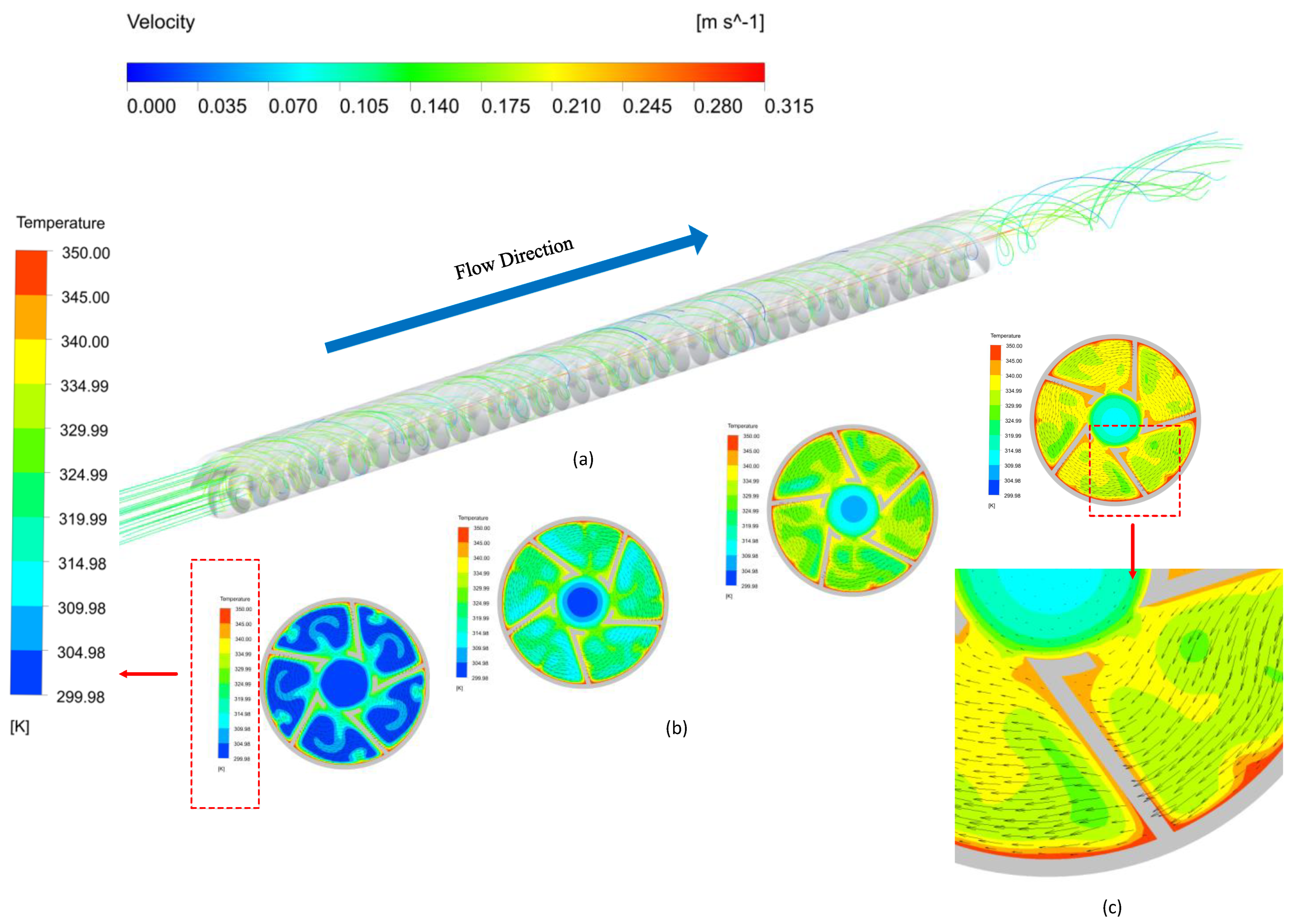
The addition of L-shaped twisted tape inserts was advantageous for enhancing fluid disturbance within the heat exchanger tube, reducing the boundary layer thickness near the tube wall, and promoting vortex formation in the L-shaped region, further enhancing heat transfer.

2.

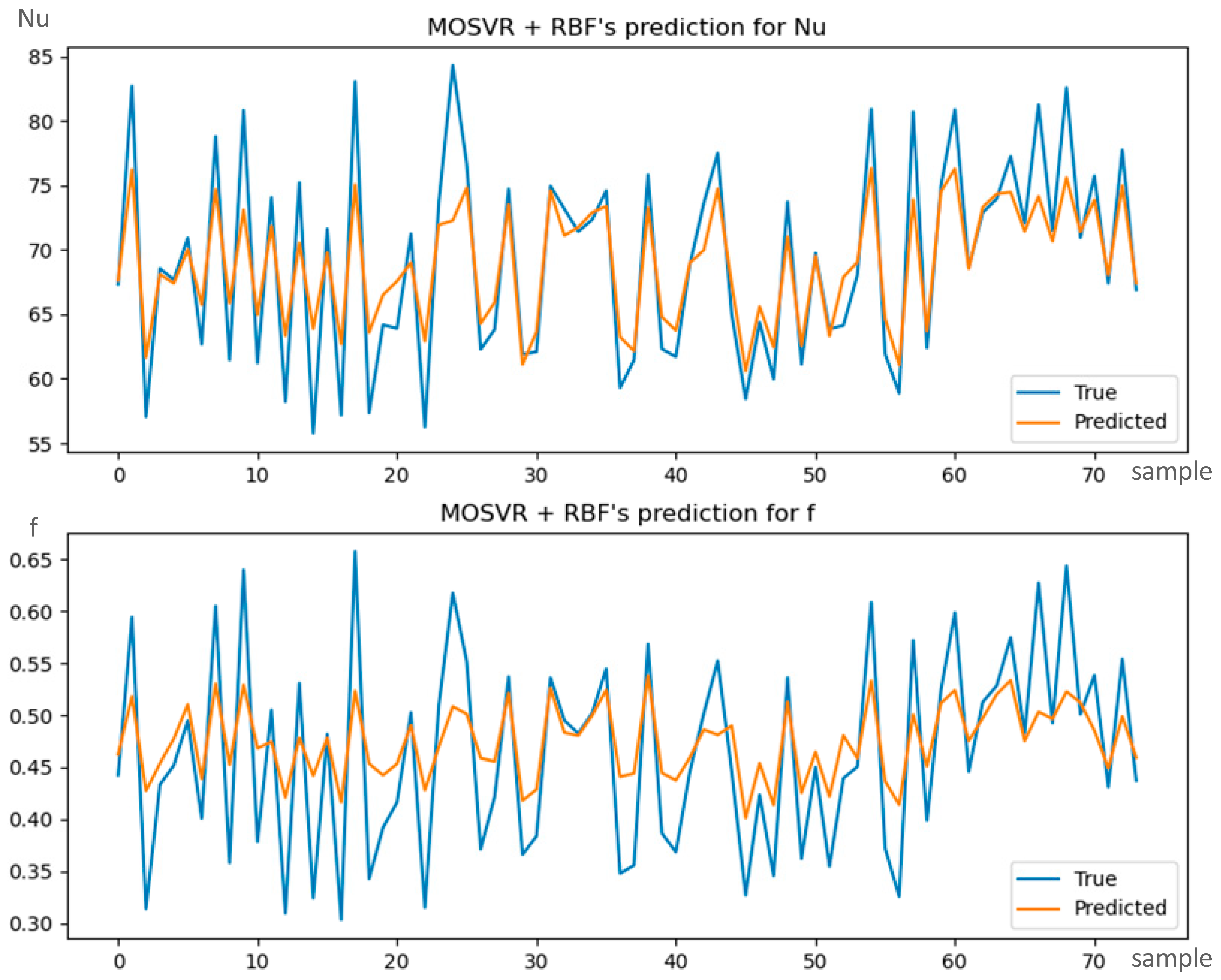
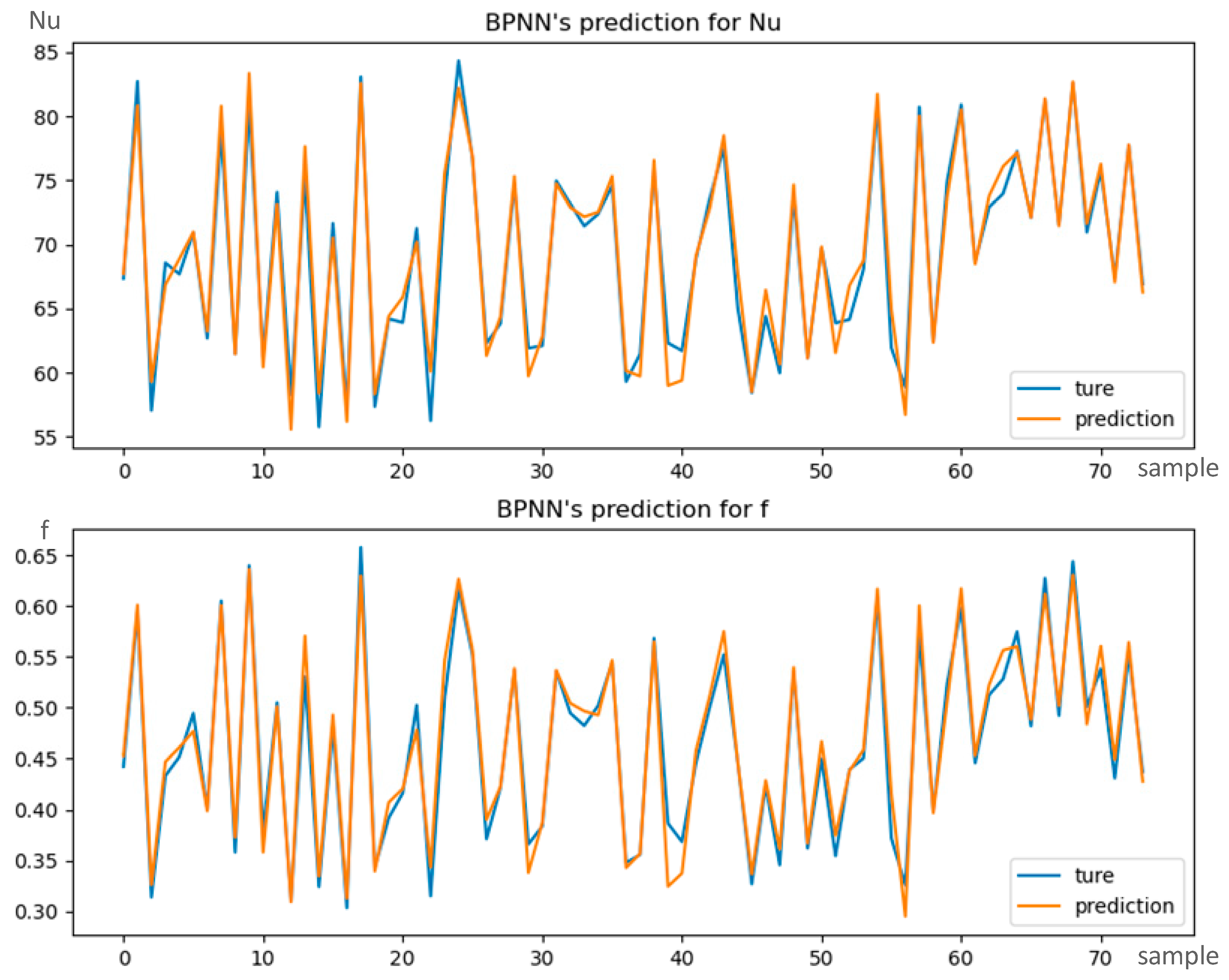
Among the four multi-output regression models, the MOGPR model yielded satisfactory results in terms of both MSE, R², and running time. The fitting performance of the BPNN model was similar to MOGPR, but with a running time twice that of MOGPR.

3.

The fitting performance of the MOLR model was inferior to the MOGPR and BPNN models, indicating that the relationship between input and output parameters was not simply linear. However, the MOLR model exhibited the lowest computational time. The MOSVR model yielded the poorest results, with performance, in terms of accuracy and error, significantly lower than the other models.

4.

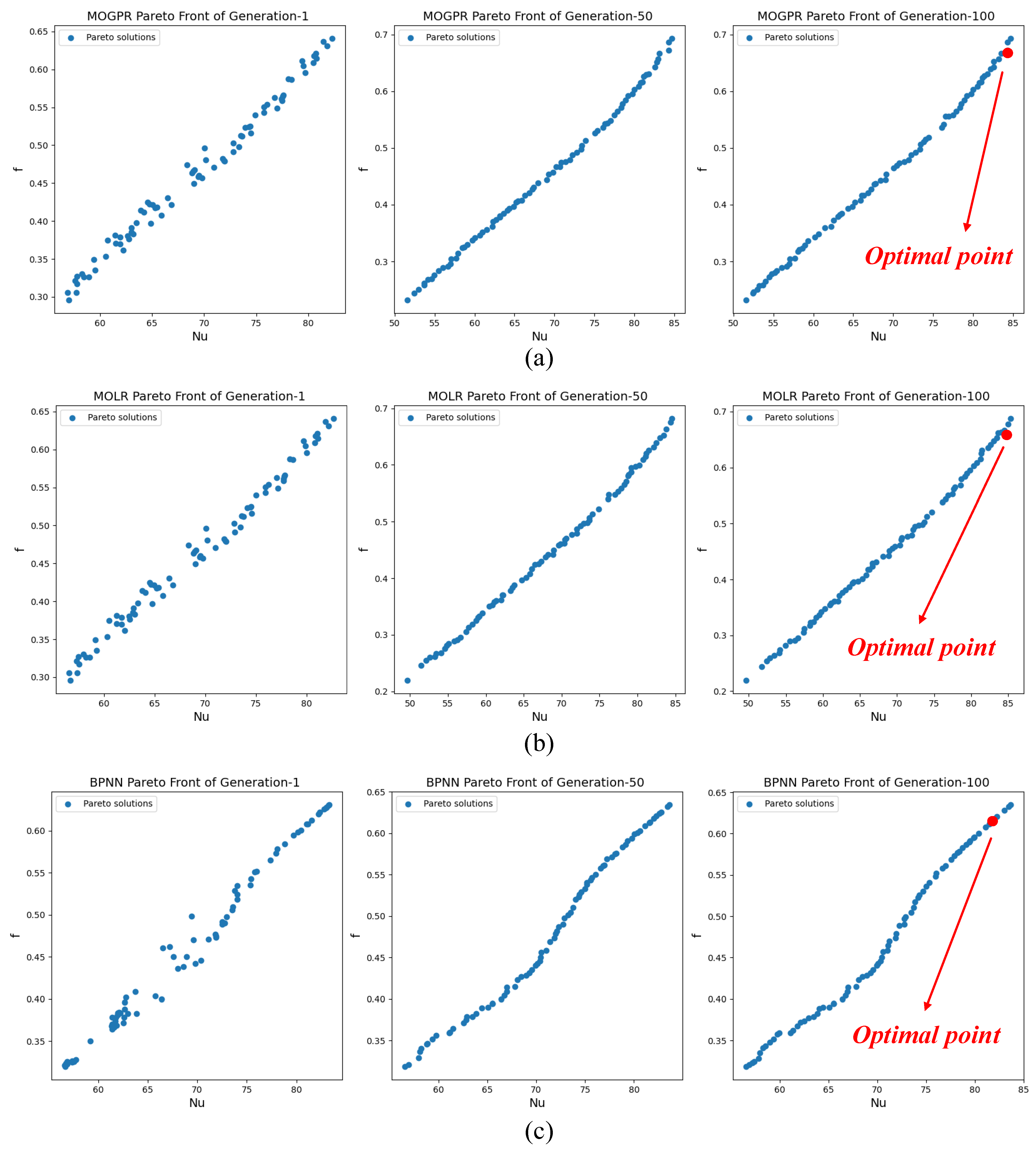
Under the guidance of various multi-output regression models, the NSGA-II method obtained a set of optimal Pareto frontier solutions, corresponding to twisted tape geometric dimensions of P = 50.50 mm, D = 6.00 mm, and W = 0.833 mm for the MOLR algorithm; P = 52.06 mm, D = 6.028 mm, and W = 0.853 mm for the MOGPR algorithm; and P = 50.12 mm, D = 6.021 mm, and W = 0.850 mm for the BPNN algorithm.

References

1. Hata, K.; Masuzaki, S. Twisted-tape-induced swirl flow heat transfer and pressure drop in a short circular tube under velocities controlled. Nucl. Eng. Des. 2011, 241, 4434–4444. [Google Scholar] [CrossRef]
2. Wongcharee, K.; Eiamsa-ard, S. Friction and heat transfer characteristics of laminar swirl flow through the round tubes inserted with alternate clockwise and counter-clockwise twisted-tapes. Int. Commun. Heat Mass Transf. 2011, 38, 348–352. [Google Scholar] [CrossRef]
3. Nalavade, S.P.; Deshmukh, P.W.; Sane, N.K. Heat transfer and friction factor characteristics of turbulent flow using thermally non conductive twisted tape inserts. Mater. Today Proc. 2022, 52, 373–378. [Google Scholar] [CrossRef]
4. Bhuiya, M.M.K.; Chowdhury, M.S.U.; Saha, M.; Islam, M.T. Heat transfer and friction factor characteristics in turbulent flow through a tube fitted with perforated twisted tape inserts. Int. Commun. Heat Mass Transf. 2013, 46, 49–57. [Google Scholar] [CrossRef]
5. Bhuiya, M.M.K.; Chowdhury, M.S.U.; Shahabuddin, M.; Saha, M.; Memon, L.A. Thermal characteristics in a heat exchanger tube fitted with triple twisted tape inserts. Int. Commun. Heat Mass Transf. 2013, 48, 124–132. [Google Scholar] [CrossRef]
6. Nanan, K.; Thianpong, C.; Promvonge, P.; Eiamsa-ard, S. Investigation of heat transfer enhancement by perforated helical twisted-tapes. Int. Commun. Heat Mass Transf. 2014, 52, 106–112. [Google Scholar] [CrossRef]
7. Van Der Merwe, A.; Zidek, J.V. Multivariate regression analysis and canonical variates. Can. J. Stat. 1980, 8, 27–39. [Google Scholar] [CrossRef]
8. Xu, S.; An, X.; Qiao, X.; Zhu, L.; Li, L. Multi-output least-squares support vector regression machines. Pattern Recognit. Lett. 2013, 34, 1078–1084. [Google Scholar] [CrossRef]
9. Brudnak, M. Vector-valued support vector regression. In Proceedings of the 2006 IEEE International Joint Conference on Neural Network Proceedings, Vancouver, BC, Canada, 16–21 July 2006; pp. 1562–1569. [Google Scholar]
10. Liu, G.; Lin, Z.; Yu, Y. Multi-output regression on the output manifold. Pattern Recognit. 2009, 42, 2737–2743. [Google Scholar] [CrossRef]
11. Borchani, H.; Varando, G.; Bielza, C.; Larranaga, P.; Discovery, K. A survey on multi-output regression. Wiley Interdiscip. Rev. Data Min. Knowl. Discov. 2015, 5, 216–233. [Google Scholar] [CrossRef]
12. Xu, D.; Shi, Y.; Tsang, I.W.; Ong, Y.-S.; Gong, C.; Shen, X. Survey on multi-output learning. IEEE Trans. Neural Netw. Learn. Syst. 2019, 31, 2409–2429. [Google Scholar] [CrossRef] [PubMed]
13. Kocev, D.; Džeroski, S.; White, M.D.; Newell, G.R.; Griffioen, P. Using single-and multi-target regression trees and ensembles to model a compound index of vegetation condition. Ecol. Model. 2009, 220, 1159–1168. [Google Scholar] [CrossRef]
14. de Lima, E.S.; Feijó, B.; Furtado, A.L. Player behavior and personality modeling for interactive storytelling in games. Entertain. Comput. 2018, 28, 32–48. [Google Scholar] [CrossRef]
15. Lopez-Martin, M.; Le Clainche, S.; Carro, B. Model-free short-term fluid dynamics estimator with a deep 3D-convolutional neural network. Expert Syst. Appl. 2021, 177, 114924. [Google Scholar] [CrossRef]
16. Bhattacharya, S.; Verma, M.K.; Bhattacharya, A. Predictions of Reynolds and Nusselt numbers in turbulent convection using machine-learning models. Phys. Fluids 2022, 34, 025102. [Google Scholar] [CrossRef]
17. Khan, M.Z.A.; Khan, H.A.; Aziz, M. Performance optimization of heat-exchanger with delta-wing tape inserts using machine learning. Appl. Therm. Eng. 2022, 216, 119135. [Google Scholar] [CrossRef]
18. Panda, J.P.; Kumar, B.; Patil, A.K.; Kumar, M.; Kumar, R. Machine learning assisted modeling of thermohydraulic correlations for heat exchangers with twisted tape inserts. Acta Mech. Sin. 2022, 39, 322036. [Google Scholar] [CrossRef]
19. Saeed, M.; Berrouk, A.S.; Al Wahedi, Y.F.; Singh, M.P.; Dagga, I.A.; Afgan, I. Performance enhancement of a C-shaped printed circuit heat exchanger in supercritical CO2 Brayton cycle: A machine learning-based optimization study. Case Stud. Therm. Eng. 2022, 38, 102276. [Google Scholar] [CrossRef]
20. Celik, N.; Tasar, B.; Kapan, S.; Tanyildizi, V. Performance optimization of a heat exchanger with coiled-wire turbulator insert by using various machine learning methods. Int. J. Therm. Sci. 2023, 192, 108439. [Google Scholar] [CrossRef]
21. Esfandyari, M.; Amiri Delouei, A.; Jalai, A. Optimization of ultrasonic-excited double-pipe heat exchanger with machine learning and PSO. Int. Commun. Heat Mass Transf. 2023, 147, 106985. [Google Scholar] [CrossRef]
22. Wang, Q.; Zhang, S.; Zhang, Y.; Fu, J.; Liu, Z. Enhancing performance of nanofluid mini-channel heat sinks through machine learning and multi-objective optimization of operating parameters. Int. J. Heat Mass Transf. 2023, 210, 124204. [Google Scholar] [CrossRef]
23. Shi, C.; Zhu, Y.; Yu, M.; Liu, Z. Arrangement optimization of spherical dimples inside tubes based on machine learning for realizing the optimal flow pattern. Therm. Sci. Eng. Prog. 2023, 44, 102065. [Google Scholar] [CrossRef]
24. Sammil, S.; Sridharan, M. Employing ensemble machine learning techniques for predicting the thermohydraulic performance of double pipe heat exchanger with and without turbulators. Therm. Sci. Eng. Prog. 2024, 47, 102337. [Google Scholar] [CrossRef]
25. Mudhsh, M.; El-Said, E.M.S.; Aseeri, A.O.; Almodfer, R.; Abd Elaziz, M.; Elshamy, S.M.; Elsheikh, A.H. Modelling of thermo-hydraulic behavior of a helical heat exchanger using machine learning model and fire hawk optimizer. Case Stud. Therm. Eng. 2023, 49, 103294. [Google Scholar] [CrossRef]
26. Li, S.; Qian, Z.; Wang, Q. Optimization of thermohydraulic performance of tube heat exchanger with L twisted tape. Int. Commun. Heat Mass Transf. 2023, 145, 106842. [Google Scholar] [CrossRef]
27. Menter, F. Improved two-equation k-omega turbulence models for aerodynamic flows. NASA STI/Recon Tech. Rep. N 1992, 93, 19930013620. [Google Scholar]
28. Argyriou, A.; Evgeniou, T.; Pontil, M. Multi-task feature learning. In Advances in Neural Information Processing Systems; The MIT Press: Cambridge, MA, USA, 2007; pp. 41–48. [Google Scholar]
29. Alvarez, M.A.; Rosasco, L.; Lawrence, N.D. Kernels for vector-valued functions: A review. Found. Trends® Mach. Learn. 2012, 4, 195–266. [Google Scholar] [CrossRef]
30. Rumelhart, D.E.; Hinton, G.E.; Williams, R.J. Learning representations by back-propagating errors. Nature 1986, 323, 533–536. [Google Scholar] [CrossRef]
31. Deb, K.; Pratap, A.; Agarwal, S.; Meyarivan, T. A fast and elitist multiobjective genetic algorithm: NSGA-II. IEEE Trans. Evol. Comput. 2002, 6, 182–197. [Google Scholar] [CrossRef]
Figure 1. Geometrical model of heat exchange tube and twisted tape insert.
Energies 17 00850 g001
Figure 2. Velocity streamline distributions of working flow at Re = 3750. (a) temperature distributions of four selected representative cross-sections, (b) velocity streamline and temperature distributions of L region (c).
Energies 17 00850 g002
Figure 3. A whole flowchart of NSGA-II.
Energies 17 00850 g003
Figure 4. A scatter plot of the simulation results.
Energies 17 00850 g004
Figure 5. Fitting performance of the MOLR algorithm.
Energies 17 00850 g005
Figure 6. The fitting performance of the MOSVR + RBF algorithm.
Energies 17 00850 g006
Figure 7. Fitting performance of the MOSVR + Sigmoid algorithm.
Energies 17 00850 g007
Figure 8. The fitting performance of the MOSVR + linear algorithm.
Energies 17 00850 g008
Figure 9. The fitting performance of the MOGPR + Matern algorithm.
Energies 17 00850 g009
Figure 10. The fitting performance of the MOGPR + Dotproduct + WhiteKernel algorithm.
Energies 17 00850 g010
Figure 11. The fitting performance of the MOGPR + RBF algorithm.
Energies 17 00850 g011
Figure 12. The fitting performance of the BPNN algorithms.
Energies 17 00850 g012
Figure 13. Pareto solution sets for different algorithms at the 1st, 50th, and 100th generations for MOGPR algorithm (a), MOLR algorithm (b), BPNN algorithm (c).
Energies 17 00850 g013