2. Equations of Motion and Development of a Time-Domain Model
This paper focuses on developing linear, stable models for the radiation force effects in single and multiple floating marine structures, such as wave energy converter (WEC) arrays, that can be used for model-based control strategies. The viscous drag forces can be ignored for the compact and sparse arrays analyzed in this work as they are small compared to radiation damping [
31]. The equations of motion shown here can be used for both hydrodynamically coupled and uncoupled arrays. A WEC array is hydrodynamically coupled when the motion of a WEC is affected by the motion of other WECs in the array. An array can be considered hydrodynamically uncoupled when its members are far enough apart to have minimal mode-couplings, the motion of any WEC in the array is independent of the motion of any other WEC.
The motion of WECs is commonly described by Equation (
1), which is the Cummins equation [
1,
2]. The viscous drag forces can be ignored for large marine structures as they are small compared to radiation damping [
2].
where the
are generalized motion coordinates, and the coefficient of
is the summation of the inertia of the system and the asymptotic added mass. That is, for an n degrees-of-freedom system,
is the inertia matrix, and
is the added mass matrix at infinite frequency. The second term is the convolution operation needed to calculate the radiation force,
. Also,
is the hydrostatic and gravitational stiffness matrix, and the
contains the Froude–Krylov, diffraction, PTO, and friction generalized forces. For a rigid body moving in six DOFs (degrees of freedom), the
are surge, sway, heave, roll, pitch, and yaw modes, and the matrices
, and
are
matrices. For multiple bodies forming an array of N rigid bodies, each moving in six DOFs, these matrices become
matrices, and the off-diagonal terms contain the appropriate coupling terms.
The linear assumptions entail that the incoming waves have small amplitude and steepness and that the body motions are also small. For the dynamics model discussed in later sections, it is assumed that no PTO or control forces are acting on the system, so the right-hand side of Equation (
1),
, will be replaced with just the excitation force,
, for the remainder of this paper. Note, in this section the excitation force coefficients and the radiation function are represented as
and
to emphasize that they are complex functions.
The excitation force is the input to the system, as shown in Equation (
2). The excitation force impulse response function (IRF) is expressed as Equation (
3). Therefore, the convolution in Equation (
2) models the excitation force acting on the system for a known wave elevation time history
, as shown in Equation (
4). The excitation force can be calculated in advance without affecting the real-time dynamic model because the excitation force depends on the incoming wave profile. However, for irregular wave inputs, with wave profiles changing in real time, prediction of the incoming wave profile becomes critical.
where
and
The second term in Equation (
1), together with the
term, corresponds to the radiation force. This term is the convolution of the radiation force IRF with the body’s velocity. This follows from defining the radiation FRF
, using the hydrodynamic radiation effects of the body, i.e., added mass
and radiation damping
, which are obtained using numerical solvers like WAMIT. The radiation FRF can therefore be expressed as
where
, such that the asymptotic added mass that converges to a constant
at higher frequencies is subtracted from the radiation function
and added to the inertia matrix
, as shown in Equation (
1). The inverse Fourier transform of
in Equation (
5) results in the radiation IRF, as shown in Equation (
6):
which becomes
Note, the radiation function
itself is a complex function; however, the corresponding IRF is a real function. This is physically justified by associating the added mass with local, evanescent, and non-propagating modes, represented by the imaginary part of the complex radiation function; while the radiation damping part propagates with the real part such that the radiation force,
, is a causal real force experienced in the vicinity. This can be shown mathematically by observing that sine is an odd function, while cosine is an even function, and that both the
and
are even functions [
2]. Therefore, the imaginary part of Equation (
7) is an odd function, thus vanishes, while the real part, being an even function, is twice its value when the lower limit is
and the upper limit is ∞. Changing the lower limit of Equation (
7) to
and doubling the real part gives
The Kramers–Kronig relations relate the added mass
and radiation damping
. The Ogilvie equations use the Kramers–Kronig relations to simplify (
8) such that
can be expressed as either a cosine transform of the radiation damping FRF
or the sine transform of the FRF of the added mass
[
32].
Therefore, the radiation IRF is real-valued and causal. Motion-dynamics modeling of a marine structure requires the convolution of Equation (
9) with the body velocity to calculate the radiation force in real time. Physically, this means the body will only experience the radiation force after a wave has hit it, and the body generates a radiation field around it that, in turn, becomes the radiation force experienced by the body. The expression for the radiation force in the time domain can, therefore, be expressed as
such that
for
. When numerically integrating Equation (
10), the limits of the integral can go from the
to
t, where
is the duration of the radiation IRF (i.e., the radiation IRF is zero for
).
3. Passivity Properties of the Radiation Function, , Radiation IRF, , and Estimated LTI System,
In its simplest high-level form, the Cummins equation is analogous to a mass–spring–damper system, where the hydrostatic forces act as a spring force while the radiation forces contribute to the damping force and the overall inertia of the system. Equation (
11) shows the equation of motion for such a 1-DOF system:
where
represents the system’s effective inertia,
z represents motion in some arbitrary mode,
the hydrostatic stiffness, followed by the convolution integral used to calculate the radiation forces, in which
is the impulse response function of the wave field radiated by the system. The right-hand side of the equation encapsulates all external forces, such as the power take-off (PTO) forces and the excitation forces. The focus of this work is identifying a linear time-invariant system that can replicate the convolution integral needed to calculate the radiation forces. This equivalent LTI system is represented hereafter as the transfer function
, where
. The Laplace transform of Equation (
11) is
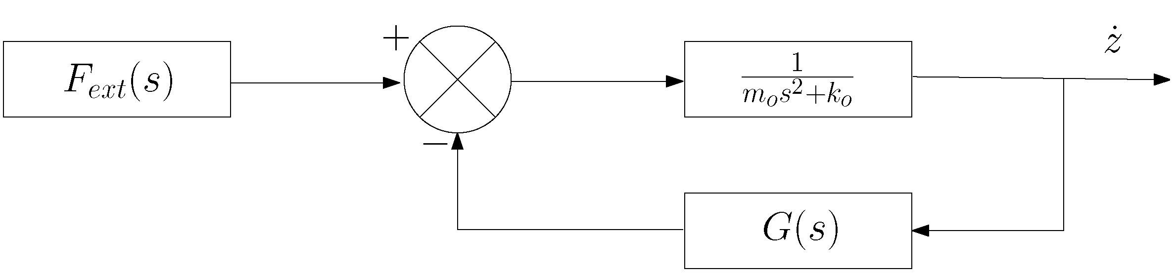
In Equation (
12), and the block diagram shown in
Figure 1, the WEC is represented as
, and is the plant of the system composed of a mass–spring system, such that
represents the mass of the simplified WEC model and
is the hydrostatic coefficient. The radiation forces serve as the negative feedback to the system, and are represented as
. The external forces, shown as
, represent the excitation forces composed of the incident Froude–Krylov forces and the diffraction forces that serve as the input to the system, and the WEC’s velocity is the output. The computation of the radiation forces requires the convolution of the body’s velocity and the radiation force impulse response function (IRF).
The radiation force is causal and needs the body’s velocity information in real time for the convolution. The radiation force in the time domain is calculated using the frequency-domain hydrodynamic coefficients, solved using a boundary element method (BEM) solver, such as commercial software packages like Wave Analysis MIT (WAMIT v7.4). The frequency-domain hydrodynamic coefficients are then used to calculate an IRF. Convolving the IRFs with the buoy velocity gives the radiation force in real time. This convolution operation makes model-based motion control difficult because motion control of a dynamic system requires the knowledge of its poles and zeros [
4,
24].
This work circumvents the convolution operation by proposing an algorithm to generate a transfer function between the radiation force and body velocity. Modeling the dynamics using a linear time-invariant (LTI) model provides the knowledge of the system’s dynamical characteristics and facilitates various motion-control strategies based on the system’s motion dynamics. Note that the model-based control schemes, whether for analysis or implementation, often rely on reduced-order models, which further necessitate system identification of the radiation forces. For instance, model-predictive control (MPC) of a WEC array is computed based on running an optimization problem at each control update step.
The motion dynamics matrices need to encapsulate all possible mode couplings. A time-domain model of a multibody system is a multiple input multiple output (MIMO) system. Estimating a linear time-invariant (LTI) MIMO system is challenging in terms of accuracy and stability. The estimated radiation force transfer function array (hereafter ) has to ensure the stability of the closed-loop multibody dynamics system. The is in the negative feedback of the overall dynamics model. A passivity-based estimation algorithm for can, therefore, ensure the stability of the overall dynamics model. A passivity-based approach also ensures fidelity to the physical system because radiation forces are dissipative in nature. The Nyquist stability criteria used for single input single output (SISO) systems can be extended to a multiple intput multiple output (MIMO) system by assessing the input passivity index () of .
The properties of radiation effects are encapsulated in the radiation function
; therefore, the estimated LTI system,
, should preserve the physical phenomenon being approximated. The boundary conditions of the radiation function
, and its time-domain counterpart radiation IRF,
, are summarized in
Table 1.
Table 1 is similar to the properties discussed by Duarte et al. and Perez and Fossen [
6,
33].
In
Table 1, properties
, and 3 are a consequence of the Riemann–Lebesgue lemma, while the BIBO stability condition in property 4 establishes the input–output stability of the convolution for radiation forces [
4,
33].
Property 5 in
Table 1 entails the dissipativity property of the radiation function
, since it starts as 0 and then converges to 0 since the radiation forces are dissipative. The Ogilvie equations indicate that the radiation IRF,
, can be calculated using the radiation damping coefficients
[
32]. The
also starts from 0 and converges to 0 since the hydrodynamic theory dictates that the
. It can be therefore said that the radiation forces are passive, since radiation forces are dissipative and they generate no energy. For linear systems, the passivity property is equivalent to positive realness [
4,
5].
The estimated transfer functions are used to calculate the radiation force and are used in the negative feedback of the complete dynamic system. A challenging property of linear systems is that even if a system such as a transfer function is stable on its own when used in the closed loop of the complete system, it can result in making the overall system unstable. Therefore, system stability can be assessed by looking into its passivity property. Passivity implies that the physical system does not generate energy and can only store or dissipate energy. Therefore, the estimated transfer function array should be passive, i.e., positive real. This stability criterion has been recognized by various researchers, such as in [
4,
6,
14,
24,
27].
The passivity condition essentially requires that the estimated LTI system,
, or the radiation force transfer function array, populated by transfer functions between body velocity and radiation force,
, is positive semi-definite, which implies that the real part of the transfer function array is positive. Formally, the passivity condition for a transfer function array, which is a multiple input multiple output (MIMO) system, can be stated as discussed by Khalil [
5].
Lemma 1. Let G(s) be a proper rational transfer function matrix, and suppose is not identically zero. Then, G(s) is strictly positive real if and only if:
- 1.
G(s) is Hurwitz; that is, the poles of G(s) have negative real parts;
- 2.
is positive definite for all ;
- 3.
Either is positive definite; or it is positive semi-definite and the terms are positive definite for any full-rank matrix M, such that the term , where . Additionally, if , then , which is the case for radiation damping.
The passivity of the estimated radiation transfer functions using the input passivity index, , is such that , where are the minimum eigenvalues of the magnitude of . For SISO LTI systems, the input passivity index corresponds to the horizontal distance of the Nyquist plot from the imaginary axis, or in other words, the real part of the Nyquist plot, since for a SISO LTI system, results in , making . Note, the passivity corresponds to the Nyquist criterion for feedback systems, requiring the phase of the LTI system in question to be within .
Classical control methods such as the Nyquist plot can be used to assess the robustness of stability and passivity. However, assessing stability through a passivity-index-based approach, as proposed here, has certain advantages, including:
Satisfying robust stability criteria such as stability, and more generally, dissipativity;
Using passivity ensures mapping the estimated LTI system to the physical properties of the system being modeled;
Passivity-based stability analysis can be extended to a MIMO system, such as a multiple-degrees-of-freedom (MDOFs) analysis of a single-body or multiple-body arrays.
Note, the evaluation of stability is based on a real quantity—the input passivity index. Interestingly, the analytic property of the radiation function is preserved when using the passivity-index-based system estimation because the estimation method matches both the magnitude and phase of the radiation function. The estimated system does eventually converge because a passive system is also dissipative, thereby preserving the analytic property of the radiation function [
34,
35]. There is, however, a trade-off between the stability of the estimated models and their fidelity to the physical system. While estimating, it must be kept in mind that, in general, increasing the order of the estimated model may result in a better fit but sacrifice passivity (and thus, stability) and also risk overfitting. Overfitting results in the estimated system having high-frequency poles (typically higher than 10
) that do not correspond to the actual physical system because marine systems are relatively very slow (typically operate within 0 to 4 rad/s). On the contrary, reducing the order of the estimated system will enhance passivity but sacrifice fidelity to the physical system being estimated.
It is proposed that the passivity property can be checked for, and the orders of the estimated transfer functions can be chosen through iterations, as discussed in [
4,
24]. Many researchers, therefore, start with the smallest order possible, i.e., relative degree 1, and then increase the order while checking for model fidelity and passivity [
4,
24]. The current state-of-the-art methods, therefore, check for passivity but do not enforce or guarantee the passivity in the estimated transfer functions [
4,
9,
20,
24].
5. Case Studies
The proposed algorithm is demonstrated using a single cylindrical buoy and a nine-buoy WEC array. The cylindrical WEC buoy represents a prototype that can be tested at a typical wave-tank facility. The incoming waves were set parallel to the
-direction. An axisymmetric body makes for a good candidate for a simpler hydrodynamic analysis. This section compares the accuracy and passivity characteristics of the estimated transfer function’s frequency response function (FRF). Falnes et al. and Folley used the non-dimensionalized hydrodynamic coefficients while discussing the radiation FRF and IRF characteristics [
31,
38]. The cylindrical WEC discussed here was modeled as a cylinder of radius 1 m and draft 1 m, such that the radius to draft ratio was unity. Therefore, for a cylinder of similar radius-to-draft ratio, the estimated transfer function can be scaled by a factor of
if the characteristic length for the cylinder of radius 1 m and draft 1 m is set to unity.
For a single WEC, the estimation process generates a
transfer function matrix
, whose diagonal elements correspond to self-interacting modes and off-diagonal elements correspond to coupled modes. This work shows the
heave mode only, but similar analyses can be carried out for other modes and mode couplings. For the single WEC case, the proposed algorithm is demonstrated using a frequency-domain route and two time-domain routes (see
Section 4.1). Henceforth, the estimated transfer function matrix will be denoted by
. The accuracy of the estimated transfer function matrix,
, is demonstrated by comparing its FRF with the radiation function
matrix constructed purely with the
heave modes and their couplings. The passivity characteristics are quantified using the input passivity index
, such that
, where
are the minimum eigenvalues of
. The accuracy of the FRF is assessed using the normalized root mean square error (NRMSE) fitness percentage, such that
where
y is the validation data, which is the magnitude of the radiation function
, while
is the FRF of the
being assessed.
5.1. A Single WEC
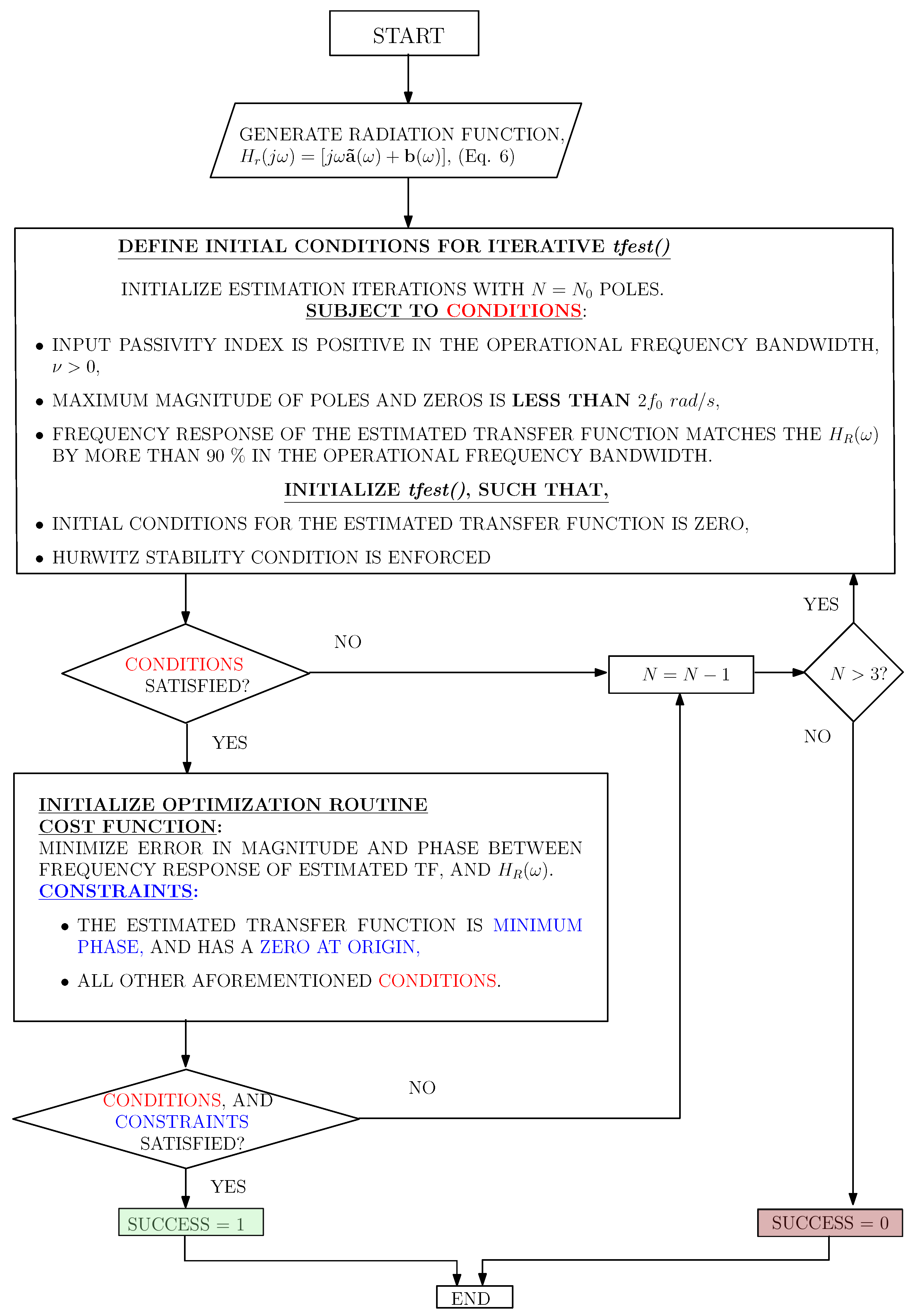
The single WEC was modeled as a cylinder of radius of 1 m and draft of 1 m, such that the radius-to-draft ratio is unity. The algorithm was initiated with
poles (see
Section 4.2 and
Figure 2). The higher-order transfer functions had high accuracy but did not satisfy the passivity requirements, while the converse was true for lower-order transfer functions. The final estimated transfer functions had satisfactory accuracy and had a positive input passivity index,
, for the frequency bandwidth in which radiation damping data from WAMIT were greater than 0.
5.1.1. Comparison of Frequency Response of Estimated Transfer Functions
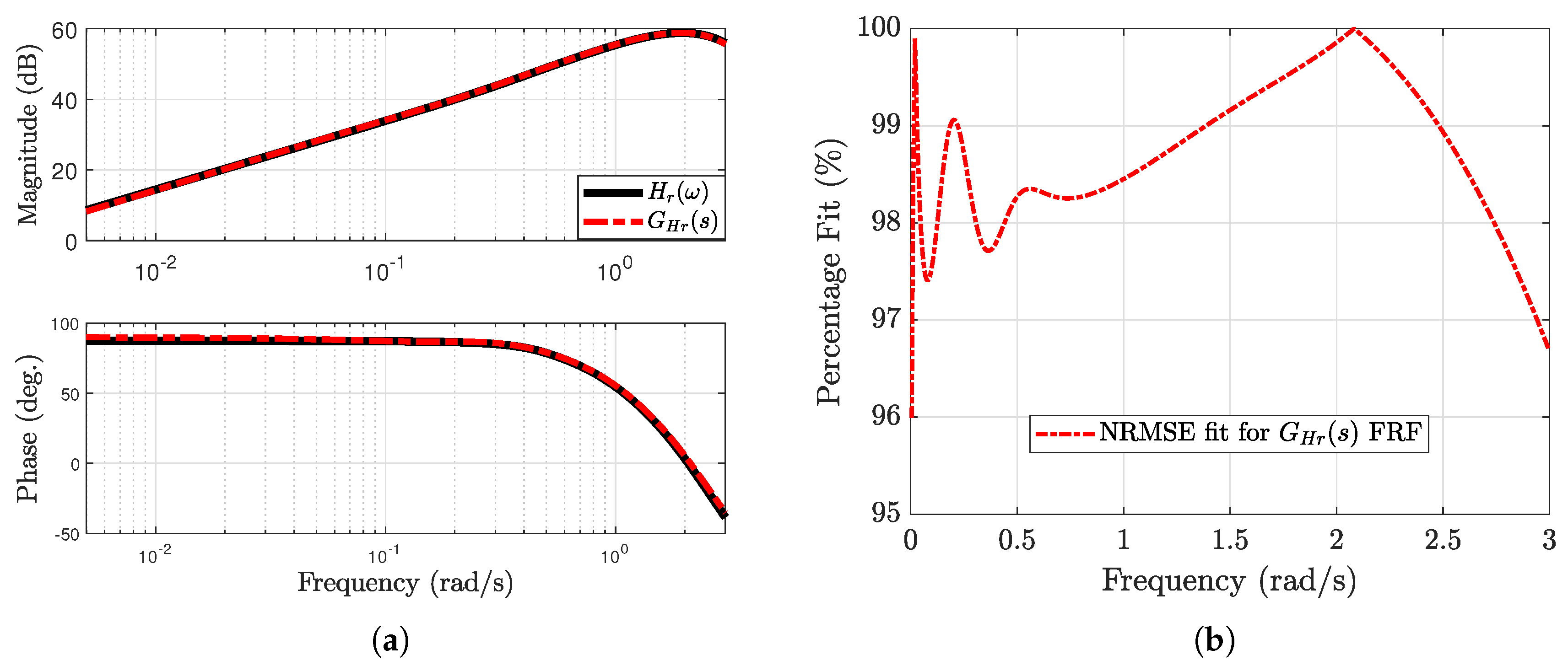
Figure 4 shows the comparison of the frequency response characteristics of
. Notice that the estimated transfer function is minimum-phase. The phase plot shows that the phase for the transfer functions stays between
, which suggests positive realness and passivity. This corresponds to the Nyquist plot being in the right-hand plane for a SISO system. The FRF of the estimated transfer functions is compared to the
. Also, the estimated transfer function has its phase plot between
. The NRMSE fit percentage as a function of frequency was calculated by comparing the radiation function
and the FRF of
.
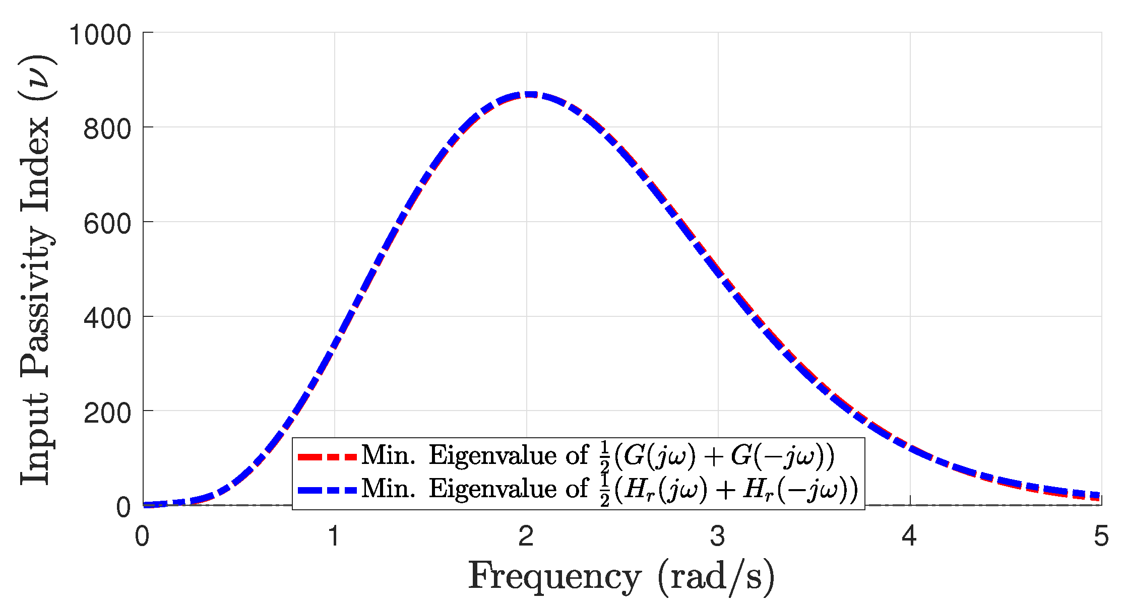
5.1.2. Comparison of Input Passivity Index of Estimated Transfer Functions
Figure 5 shows that the estimated transfer functions have a positive input passivity index between 0 and 5 rad/s. Therefore, the estimated transfer functions will have passivity for the frequency bandwidths where
is positive. Since this work is only using the heave mode, the transfer function system is a single transfer function corresponding to that mode, and therefore, the input passivity index reduces to the FRF of the corresponding estimated
. In other words,
for SISO LTI systems. Note that for multi-mode analyses such as MDOFs systems or multibody systems, the transfer function system will be a MIMO transfer function matrix and, therefore, will not reduce to
. As discussed in
Section 3, stability analyses can also be performed using the Nyquist criterion; however, it is limited to SISO systems. As described in
Section 4, the final optimization routine ensured that the estimated transfer function had a positive input passivity index in the operational bandwidth, had high accuracy with respect to the corresponding radiation function, and had a
zero at the origin (see
Table 1). The input passivity index analyses shown here make the stability analyses simpler, especially for MDOFs and multibody systems, as shown in the following subsection.
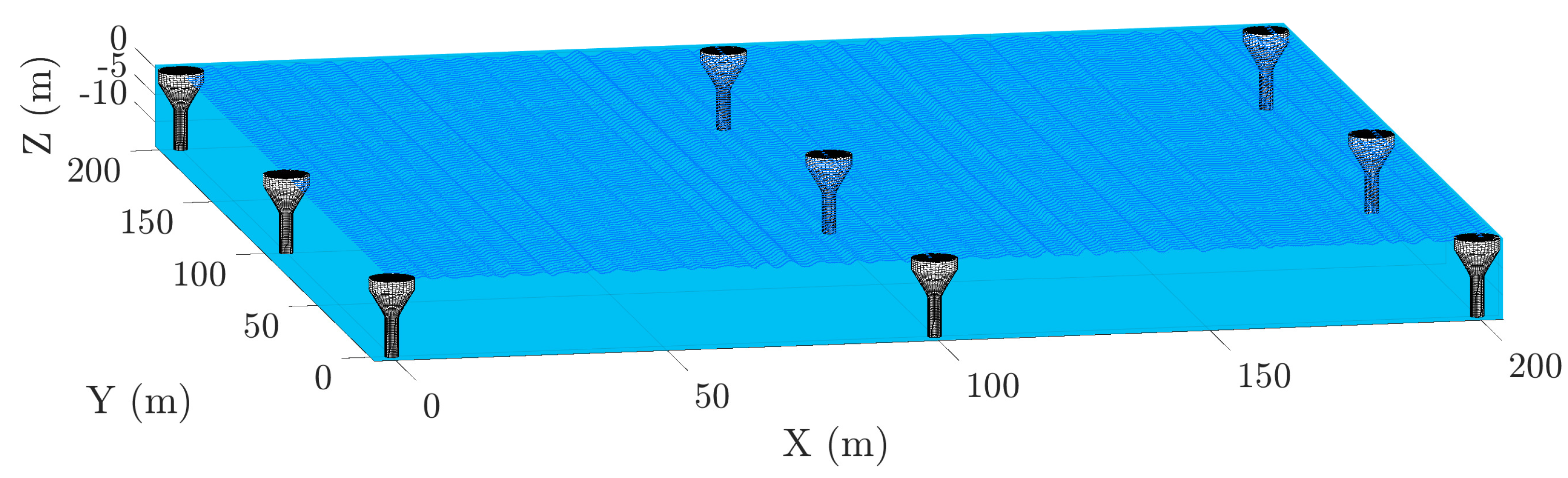
5.2. A Homogeneous WEC Array of CorPower Devices
The algorithm will now be demonstrated using a homogeneous array comprised of nine CorPower devices laid out in a square array of three rows and three columns (see
Figure 6). The CorPower is a heaving point absorber device being developed by the Swedish company CorPower Ocean and its device specifications can be found at [
39]. The device can be described as a combination of three shapes: a cylinder of diameter
m and height
m over an inverted-truncated cone with top radius
m, bottom radius
m, and height
m. The third and bottom-most part of the device extends as a cylinder of radius
m for a length of
m. The draft of the device is
m.
This homogeneous WEC array was designed to represent a realistic deployable compact array. The distance between any two neighboring bodies was 100 m along the
directions. The hydrodynamics were calculated assuming plane-progressive waves propagating along the positive
X-axis.
Figure 6 shows the homogeneous WEC array’s spatial layout. For a WEC array, the self-interacting modes and their mutual couplings result in a
radiation function matrix (where
for the current array). For this work, only the
heave modes and their mutual couplings are considered, such that the radiation function matrix was an
matrix.
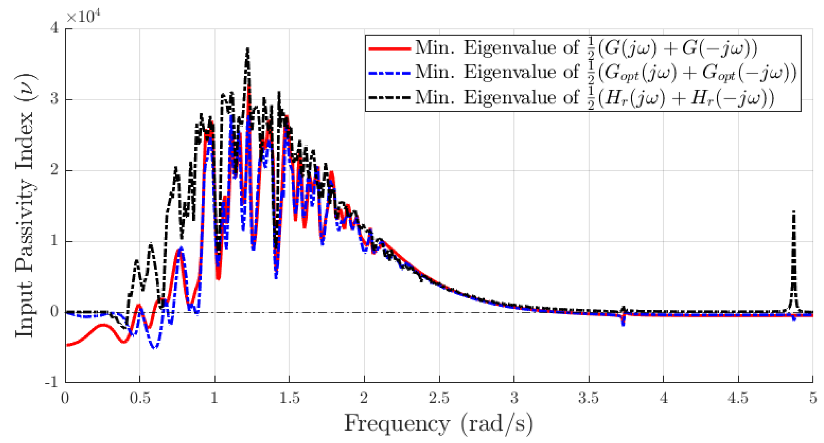
5.3. Passivity Index, , for the Homogeneous WEC Array
The WECs in the homogeneous array had a much higher volume (16 times that of the cylinder in the previous case), and the WECs in the array interacted with each other such that the motion of one WEC affected another due to hydrodynamic coupling. The multiple peaks in the passivity index of the homogeneous array in
Figure 7 indicate hydrodynamic couplings in the system.
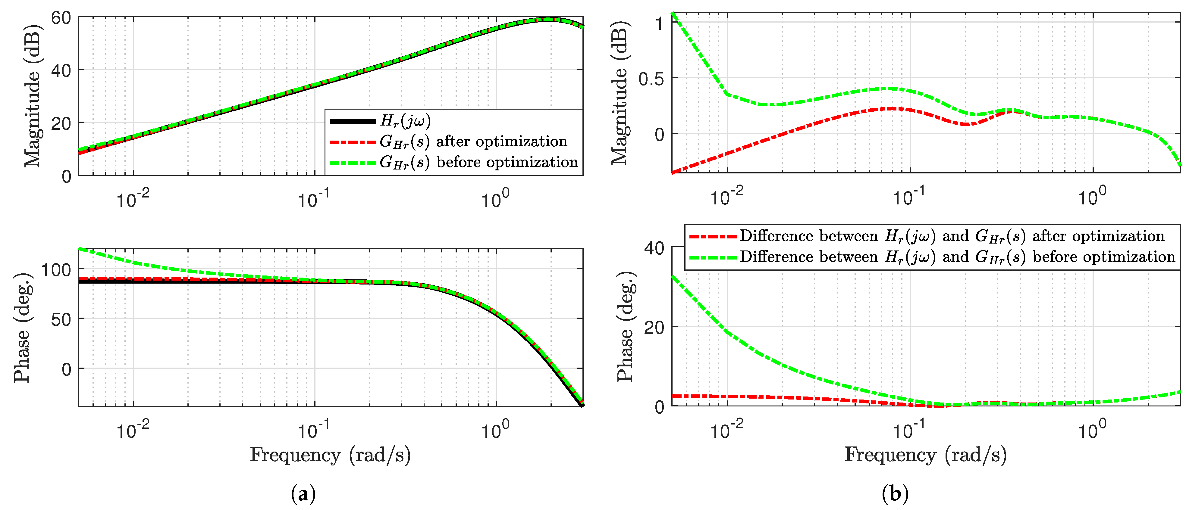
It can be observed in
Figure 7 that the optimized transfer function matrix represented by
shows an increase in the input passivity index, especially at lower frequencies. The optimization also ensured that the phase at 0 rad/s was
for all transfer functions in the transfer function matrix. Note, a phase of
at 0 rad/s indicates a zero at the origin. All estimated transfer functions matched with the corresponding reference radiation function by more than 90 % in terms of NRMSE error defined in the previous case. The asymptotic convergence to
zero indicates that the estimated transfer function matrix represents a dissipative system. The input passivity index characteristics shown can be used to inform WEC array design and optimize a control strategy that can maximize the energy extracted. The properties mentioned in
Table 1 were, therefore, achieved by the proposed system identification algorithm.
7. Discussion
The frequency domain was used to estimate transfer functions between body velocity and radiation forces. Frequency-domain estimation methods are the most direct route to generate the desired time-domain models. Marine systems operate at relatively low-frequency bandwidths. For instance, JONSWAP and Bretschneider wave spectra have most of their energy concentrated between 0 and
rad/s [
1,
2,
31]. Due to the relatively slow nature of marine dynamics and very narrow bandwidth of marine systems, the FRF of a marine system encapsulates critical information about the said marine system’s dynamics at each data point in the FRF. Direct estimation methods, like the frequency-domain estimation method shown here, can reduce the potential numerical artifacts that multi-stage time-domain estimation methods may have due to truncation and round-off errors. The proposed algorithm can achieve highly accurate transfer functions using the direct estimation or frequency-domain route despite its sensitivity, while having a positive input passivity index across most of the operational bandwidth.
As discussed in
Section 4.2, the proposed algorithm tries to strike a balance between the accuracy of the estimated transfer function and its passivity characteristics by iterating upon the order of the estimated transfer function system. Empirically, increasing the order of the estimated transfer function system increases its accuracy while decreasing its passivity and vice versa.
The estimated models were assessed based on two metrics; firstly, how well the estimated models replicated the FRF of the radiation functions, and secondly, how well was the body motion replicated when the radiation force was calculated using the estimated models as opposed to calculating the radiation force using the convolution approach. Significantly, the estimated LTI systems presented here did not have high-frequency poles, despite being high-order systems. Low-order estimation methods compromise the fidelity of fit in favor of stability and robustness, resulting in underfitting, as was the case in [
4,
24]. Conversely, high-order estimation methods compromise guaranteeing stability and robustness because they have poles faster than the physical system’s properties due to overfitting [
4,
24]. The proposed estimation algorithm succeeded in preventing underfitting and overfitting while guaranteeing Hurwitz stability and ensuring passivity. Although Taghipour et al. observed that the body motions tend to be less sensitive to the otherwise sensitive LTI system estimation process [
4], an effective and optimal motion-control design requires that the model-based controller be based on the physical phenomenon’s most accurate representation. Therefore, sacrificing accuracy in favor of passivity should be assessed based on the particular case being considered.
The case studies that are shown here demonstrate that the proposed algorithm can model accurate and stable motion-dynamics models of MDOFs marine systems with various degrees of hydrodynamic coupling. The off-diagonal terms representing the coupled modes of the radiation function are highly oscillating but have relatively low magnitudes. These terms were modeled with relatively higher-order transfer functions due to the sensitivity of the coupled modes. Their low magnitude and highly oscillatory behavior make the transfer function estimation more challenging. It could be argued that the low magnitude and highly oscillatory behavior of these terms is non-physical and due to numerical issues in the calculation of the hydrodynamic coefficients corresponding to the inter-body hydrodynamic couplings.
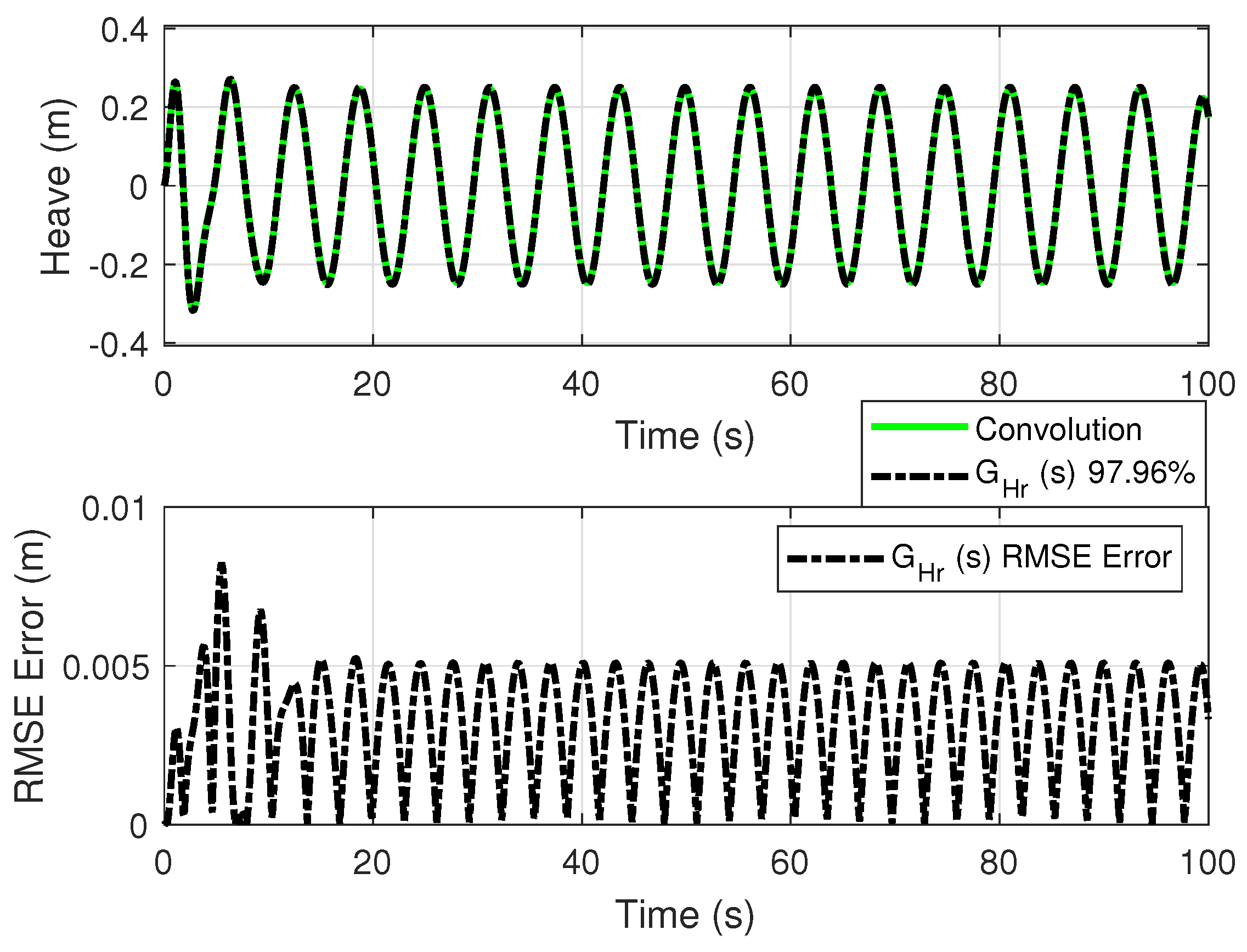
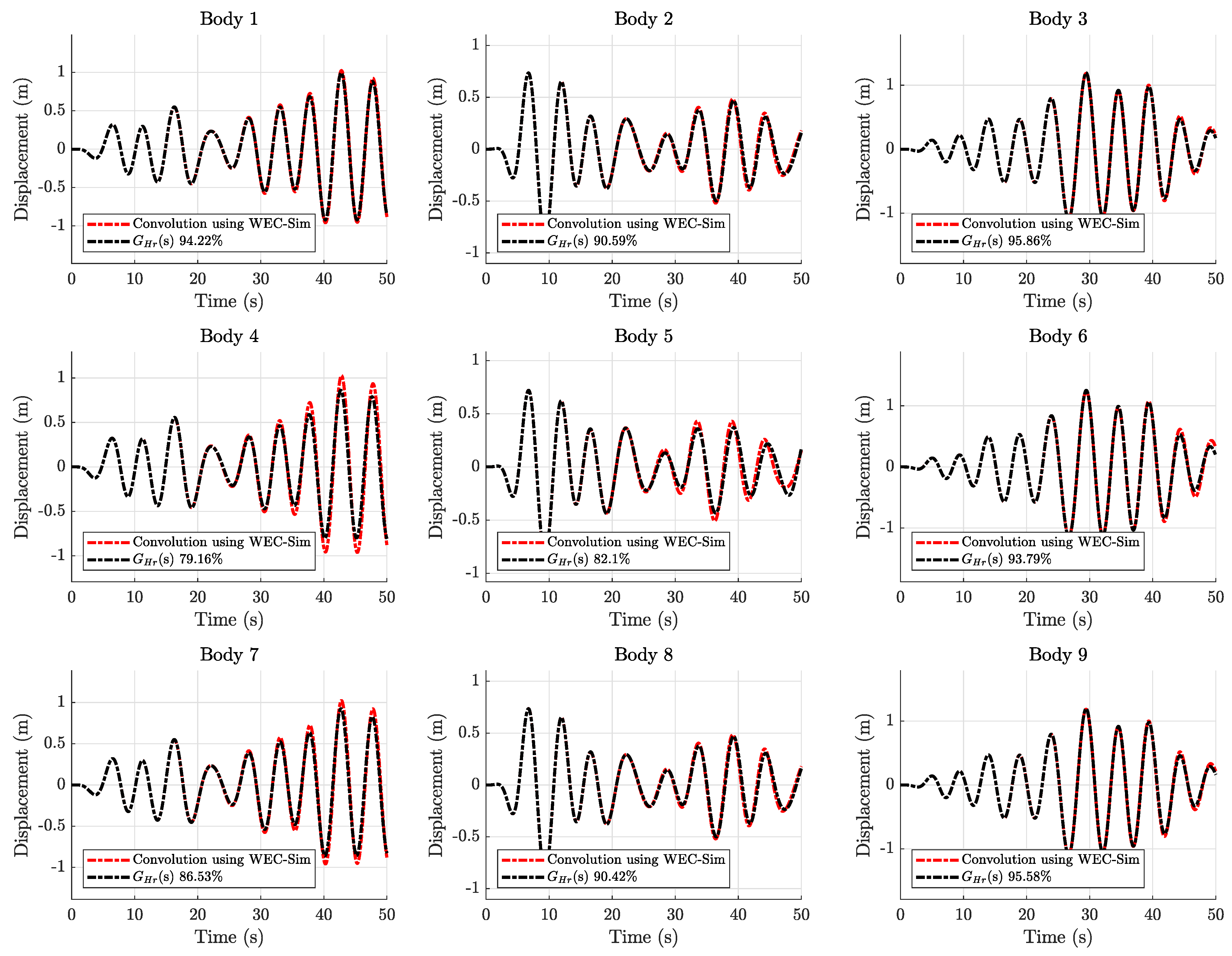
The motion time histories from the models using the convolution-based radiation forces were used as the reference for the time-domain performance of the models using the estimated transfer function array to calculate the radiation force. Ultimately, the body motion characteristics should replicate the motion characteristics calculated using Cummins’ equation. As shown in
Section 6, all cases resulted in very accurate motion characteristics while staying stable. A numerically stable time-domain model that can be analyzed in the Laplace domain using the estimated LTI systems can eventually be used to investigate the multibody dynamics of more complicated models with the necessary control.


