Article

Potential Analysis and Feasibility Study on the Hydrothermal Utilization of Rivers—Using Marburg on the Lahn River as Case Study

Department of Civil and Environmental Engineering, Technical University of Darmstadt, 64287 Darmstadt, Germany
*
Author to whom correspondence should be addressed.
Energies 2024, 17(1), 36; https://doi.org/10.3390/en17010036
Submission received: 22 November 2023 / Revised: 13 December 2023 / Accepted: 18 December 2023 / Published: 20 December 2023
(This article belongs to the Topic Sustainable Thermal Energy Technologies and Processes)

Abstract

:
Due to their high specific heat capacity and constant thermal regeneration through flow, rivers are a promising renewable environmental heat source. The suitability of a river for hydrothermal use depends on river section-specific and site-specific factors. This paper presents a methodological proposal for a river section-specific potential analysis and site-specific feasibility study. The presentation of measured values in the form of hydrographs and duration curves as well as the use of suitable mean values and confidence intervals are central steps in the evaluation. The application of the potential analysis showed that the discharge in particular influences the size of the heat potential, while the water temperature determines whether and how the hydrothermal use is possible. The focus of this work was on the analysis of water temperature. Its significance for hydro-thermal use is multi-layered, and an assessment should be carried out at different levels. Using two specific sites on the Lahn river as a case study, the feasibility study method is demonstrated in this paper.

1. Introduction

Heat pumps are used to harness renewable heat from the environment for heating purposes and to provide hot water. They can raise the temperature level of the extracted environmental heat to the required temperature level by supplying electrical energy. Due to the high specific heat capacity of water (cp,water ≈ 4.2 kJ/(kg·K)), rivers offer an efficient way of utilizing environmental heat. This means that more heat can be extracted per Kelvin of cooling from water than from air (cp,air ≈ 1.0 kJ/(kg·K)) and most other natural fluids. For the same reason, water temperatures react more slowly than air temperatures and have higher average values in winter [1]. The continuous flow of water ensures the regeneration of the heat source. The heat potential of a river can be described by the following formula [2]:
Q ˙ t h = ϱ w · c p , w · Q r i v · T
  • Q · t h : Thermal output in kW;
  • ϱ w : Density of water in kg/m3;
  • c p , w : Specific heat capacity in kJ/(kg∙K);
  • Q r i v : Discharge of the river in m3/s;
  • T : Difference between original and changed water temperature in K.
The choice of temperature reduction is decisive for the type of heat potential. In principle, the physically available, the permissible, and the utilized heat potential can be differentiated (see Figure 1). A body can be cooled down to absolute zero. From the physical point of view, cooling to the freezing point is interesting, as this is heat extraction from a body of water with a liquid medium (physically available heat potential). As cooling to freezing point carries the risk of damage to the system due to ice formation and as the temperature difference should be limited for ecological reasons, the permissible potential (see Section 3.1.3 and Section 3.10) reflects the heat extraction that is legally and technically feasible. Heat extraction systems do not fully utilize the permissible potential, as the heat extraction rate of the systems are not sufficient, and not all of the heat potential is required. The amount of heat actually extracted is the utilized potential.
There are basically two heat extraction systems (see Figure 2): the open system and the closed system [3]. The open system extracts water from the river, passes it through the heat pump’s evaporator, and then returns it. This system has low energy losses but is only suitable for bodies of water with high water quality and a low risk of ice formation. The closed system separates the evaporator from the river and uses a heat exchanger with a heat transfer circuit to absorb the heat and transport it to the heat pump. Due to the system separation, this system has higher energy losses (approx. 1 K heat loss [2]) but is more resistant to contamination and ice formation.
The suitability of a river for thermal use depends on factors specific to the river section and site, which are shown in Table 1. The influencing factors are summarized in three categories:
  • The macroscopic level, where the heat potential of the river section is considered (potential analysis);
  • The microscopic level, where the usability of the river heat at the individual site is concretized (feasibility study);
  • The economic level, where the feasibility of the supply targets is assessed on the heat sink side.
A comprehensive analysis of these factors is necessary in order to assess the usability of river heat. There is literature in which heat potentials are determined. In particular, the researcher Adrien Gaudard from the ETH Zurich (Water Research Department) and his colleagues developed a general framework for the use of surface water heat and, based on this, also determined heat potentials in Switzerland, both over large areas [2] and at specific locations such as Lake Walen [5], Lake Brienz, Lake Thun, and Lake Biel [6]. The British Department of Energy and Climate Change also carried out a large-scale potential analysis on England’s rivers [7]. The Department of Economic, Social, and Environmental Affairs in Basel-Stadt determined the heat potential of the Rhine [8]. The heat potential of the Danube was investigated at two locations as part of a master’s thesis at the University of Freiburg [3]. As part of a district heating study for Berlin North Neukölln, the river heat potential of the Landwehr Canal was investigated [9], referring to the information sheet for the water law approval of the city of Deggendorf [10]. The conditions for heat extraction, such as the minimum temperature after heat extraction, the maximum temperature change in the river, and the assumed discharge, varied in each case. The paper addressed the different conditions and propose a comprehensive approach. In addition, the paper aimed to include the feasibility study alongside the potential analysis. This involves other parameters of the river and the river environment than water temperature and discharge. These parameters influence whether river heat utilization is even possible at the respective location. Gaudard [11] and Marotz [1,12] also dealt with other parameters in passing.

2. Materials and Methods
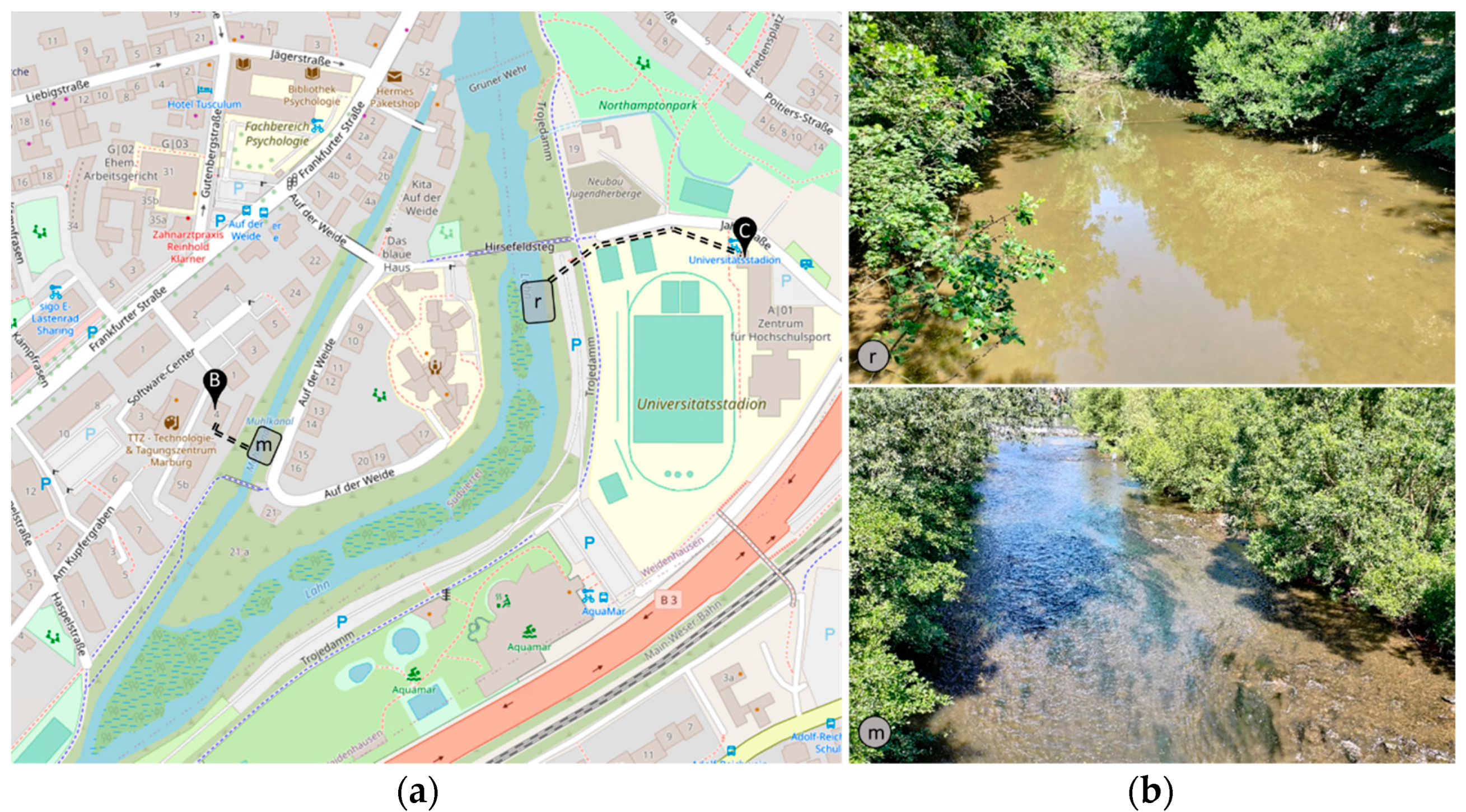
2.1. Case Example

The influencing factors on the heat potential of the river section (macroscopic level) are generally dealt with for the Lahn river in Marburg. The influencing factors at the microscopic level and the level of the heat sink require specific sites in order to be able to carry out an analysis of the feasibility of river heat utilization. As a case study, sites on the Lahn river in Marburg, Germany (see Figure 3) were analyzed for their suitability for hydrothermal utilization. The Lahn river stretches a distance of 242 km, navigating through three federal states of North Rhine-Westphalia, Hesse, and Rhineland-Palatinate, where it finally drains into the Rhine river. The river section under consideration is assigned to the barbel region (epipotamal, summer-warm).
Site 1. “Wehrda waterworks” (see Figure 4): The Wehrda waterworks of Stadtwerke Marburg GmbH are located in Wehrda. As part of the construction of the new waterworks, transport pipelines for the extraction of river water heat can be considered. Upstream of the waterworks is the Wehrda weir, which dams up the Lahn river, originally to generate electricity from a hydroelectric power plant. The turbine has been shut down and the associated siphon system is no longer active. This means that there is practically no current in the millrace.
Site 2. “Softwarecenter heat network” (see Figure 5): This site is located downstream of the Grüner weir. The operational areas are in the millrace and in the main channel of the river. Connection points B and C for heat extraction are intended to feed the river heat into the local heat network of the public utilities.

2.2. Data Procurement

If a feasibility study on hydrothermal energy is to be carried out, the data required to analyze the influencing factors in Table 1 must first be obtained. A basic distinction is made here between measurement data recorded over a period of time and static information. The measurement data for the Marburg case study is located in Figure 6 and listed in Table 2.

2.3. Statistical and Further Analysis Methods

2.3.1. Averaging the Measurement Data
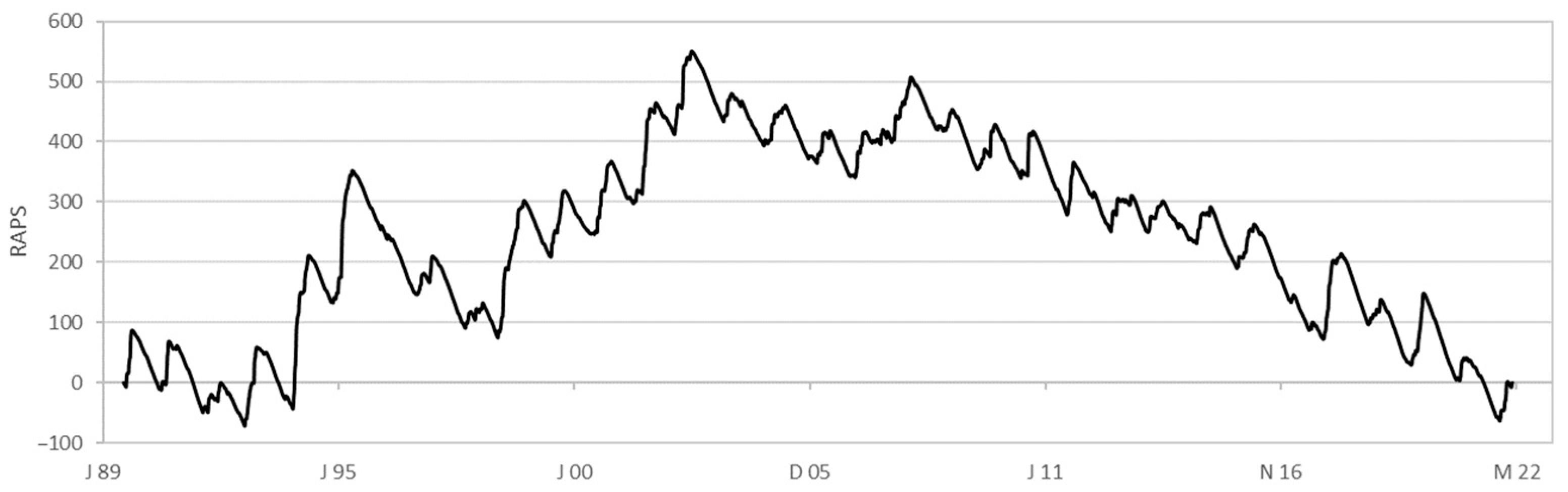
Two options are available for averaging measured values: The median is suitable for short observation time series with possible extreme values in order to reflect the average behavior of the population [13]. The arithmetic mean is suitable for longer series. The reliability of statistical statements is closely related to the length of the observation period, whereby periods of 20 years or more are considered useful in the statistical analysis of flood discharges (20 to 30 years = conditionally suitable; >30 years = suitable) [14]. In this paper, the median was used for periods of less than 20 years and the arithmetic mean for periods of 20 years or more. The 15th and 85th percentiles were used for the lower and upper confidence intervals, based on the German Climate Atlas of the DWD. The percentiles can also be used as future change corridors when considering climate ensembles [15].

2.3.2. RAPS Method

Where trends and irregularities of time series are not visible in their representation over time, particular time series analysis methods help. The Rescaled Adjusted Partial Sums (RAPS) method is appropriate for time series analysis in hydrology, like for river flow and water temperatures [16]. This method eliminates the concealing effect of the mean and variability of the data by rescaling the variable and summing the resulting departures about the mean over time [17]. Due to the summation of consistent small departures spanning several time increments, large cumulative departures can be recognized. The following equation defines the RAPS values:
X k = j = 1 k Y j Y ¯ S Y ; k = 1 , , n
  • X k : RAPS value of current summation;
  • Y j : Value of time series at time point j;
  • Y ¯ : Sample mean;
  • S Y : Standard derivation;
  • k : Counter limit of current summation.

2.3.3. Cross-Correlation

The similarity between two time series is expressed by the cross-correlation coefficient as a function of the time shift τ. If the values of the two time series are similar but shifted by the time interval τ, then the cross-correlation for τ will show a maximum. The correlation coefficient |Rxy| has a value of 1 for a complete dependency. If the value is 0, however, then there is no dependency [13].

2.3.4. Duration Curve (Underrun Days)
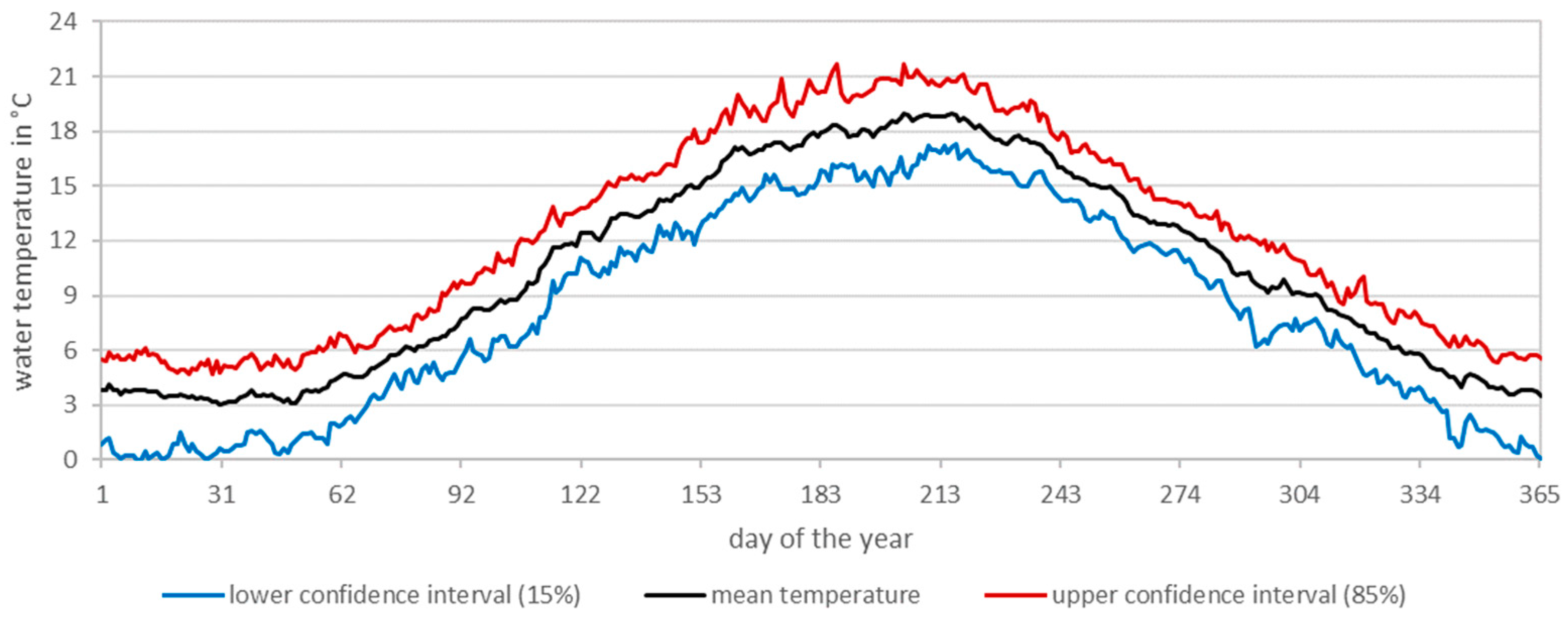
The duration curve represents measured values (individual values or classes) in ascending or descending order and corresponds to the cumulative frequency polygon. The area under the duration curve is equal to the mean value for the period under consideration. The duration number (value of the abscissa) indicates how often a certain value is underrun (underrun duration) or overrun (overrun duration). Annual duration curves of daily water levels and discharges are published in yearbooks.

2.3.5. Typical Year

The so-called test reference years represent location-specific time-averaged meteorological parameters over a year and are thus intended to represent a typical weather condition for the year. Based on this, a typical year was determined in this paper using the measurement data of a parameter (e.g., water temperature). The long-term measurement data were averaged for each day of the year, and their upper (85%) and lower (15%) confidence intervals were specified. This is intended to describe a typical average annual pattern with probable fluctuations for the respective parameter.

2.3.6. Contribution of Heat Consumption

Heat consumption in private households depends on the outdoor temperature. In order to map an annual profile of the heat consumption, the degree days and the sum of degree days were determined in accordance with German VDI Guideline 3807, Sheet 1 (Verein Deutscher Ingenieure/Association of German Engineers, Düsseldorf, Germany) (20 °C standard indoor temperature, 15 °C heating limit temperature). The daily ratio of degree day to the sum of degree days then indicates the percentage of daily heat consumption.

3. Conducting the Potential Analysis and Feasibility Study

In this section, the influencing factors according to Table 1 are explained and applied to the case study. The first two influencing factors relate to the entire river section in Marburg (macroscopic level), while the other influencing factors are explained on the basis of specific sites (microscopic level) or in general. The focus of this work is on water temperature.

3.1. Water Temperature (Macroscopic)

The evaluation of water temperature for the use of river heat is complex and takes place at different levels. Figure 7 shows the levels and in which subchapter the aspects are dealt with (generally from left to right).

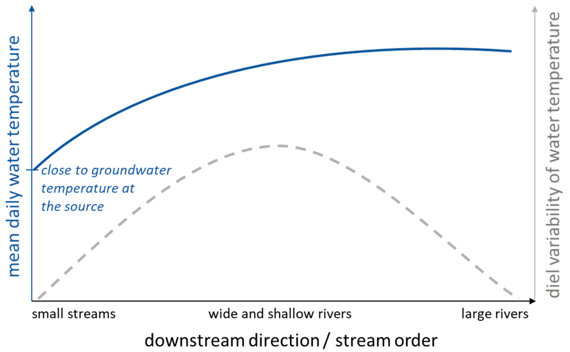
3.1.1. Characteristics: General Changes

Characteristic changes in water temperature can be seen both temporally and spatially, the cause of which lies in the thermal balance of rivers (see Figure 8). Topography, atmospheric conditions, streambed, and stream discharge as influencing groups affect the heat exchange processes involved and thus influence the thermal regime of rivers [18]. Figure 9 shows the resulting temporal and spatial variability of the water temperature.
Near the river source, the water temperatures roughly correspond to the groundwater temperature. The average daily water temperatures rise in the direction of flow, although this increase varies depending on the river (see Figure 9). For smaller streams, it is about 0.6 K/km, while for larger rivers, the increase is slower, about 0.1 K/km. In addition, the temperature varies depending on the shape of the river [18]. In terms of time, a distinction can be made between the annual and daily cycle. Within a day, the water temperature reaches its minimum in the early morning, rises until late afternoon, and then falls again (see Figure 9). Daily temperature fluctuations vary depending on the river shape. The annual cycle shows a sinusoidal course; in the moderately cool climate zone, the daily mean temperature rises from spring to its peak and falls again from early fall.
In addition to natural fluctuations, water temperature also changes due to climate change. In 2013, a study using simulations of the IPCC emission scenario SRES B1-A2 and a global physically based hydrological-water temperature modeling framework concluded that the global average temperature of rivers for the period 2071–2100 will rise by an average of 0.8 K to 1.6 K compared to the period 1971–2000 (0.08 K to 0.16 K per decade) [19]. The highest temperature increases are expected for the USA, Europe, eastern China, and parts of Africa and Australia [19]. Another study found that the temperature of rivers in England and Wales rose by an average of 0.52 K between 1990 and 2006 (0.3 K per decade) [20]. The European Environment Agency analyzed the temperature changes of the three major European rivers Rhine, Meuse, and Danube over the last century and observed an increase in water temperature of around 1 K to 3 K (0.1 K to 0.3 K per decade) [21]. In the 21st century, a temperature rise of 3 K to 3.5 K is expected in the Rhine (0.3 K to 0.35 K per decade) [21].
Various measuring stations along the Lahn river in Marburg were used to analyze the temperature curve (see Figure 10). These measuring stations showed similar seasonal patterns, with water temperatures generally rising from spring to August and falling from August to February. The measuring stations showed a close correlation of R = 0.94. They showed smaller temperature increases than indicated by Caissie [18] (see Table 3).
The temperatures measured at the Wehrda waterworks were plausible according to Figure 10 and were highly representative due to a high measurement interval and a large amount of data. The temperature differences along the Lahn river were relatively small. Therefore, the water temperatures at the Wehrda waterworks were used as representatives for the entire study area. Using the RAPS method, it can be seen that the temperatures show a trend (see Figure 11). The parabolic shape of the RAPS values indicates a continuous unidirectional temperature trend caused, for example, by urbanization or a gradually changing environment, like one affected by climate change [17]. Here, temperatures rose over time. From spring 2011, the RAPS values rose faster than they previously fell. This indicates a slight shift [17]. There may have been a change in instrumentation here or climate change could no longer only be reflected in a linear rise in temperature.
The characteristic course of the year showed an increase in the mean water temperature from the minimum tmin = 3.0 °C in February to the maximum tmax = 19.0 °C in August (see Figure 12). The coldest values of the lower confidence interval were at the freezing point in winter, while the upper confidence interval showed a minimum of 4.7 °C.
A British study produced a heat map (surface waters), not on the basis of daily averages but of three-month averages from December to February [7]. Although this may be adequate for comprehensive studies, it does not consider any underrun days (see Section 3.1.4), which can be decisive in assessing the usability of river heat. Furthermore, the water temperatures were interpolated along the watercourse and further calculated with the interpolated temperature values at the gauge for discharges. For Marburg, it was assumed that the spatial temperature changes within Marburg were not significant and were therefore considered constant (see Figure 10 and Table 3).

3.1.2. Characteristics: Thermal Discharge

Anthropogenic factors, such as thermal wastewater and water extraction, play an important role in the heat balance of rivers (see Section 3.1.1). This includes wastewater from sewage treatment plants, commercial and industrial operations, power plants, as well as mine and sump water. The discharge of heat into rivers can increase their temperature level and thus make them more suitable for hydrothermal uses. However, when planning river heat plants, it must be taken into account that a future reduction or cessation of thermal discharges can lead to the cooling of the water, which could have a negative impact on the economic operation of the plants.
In this case study, it was investigated whether thermal discharges are present along the river section under consideration and whether they have a thermal impact on the river. There is one known thermal discharger in Marburg: a manufacturer of aluminum and plastic products. Compared to the heat potential of the Lahn river, the heat input from the wastewater is negligible (see Table 4). Based on the lowest heat potential of the Lahn river in the summer months (50 MW), the heat input corresponds to only 1.6% of the Lahn river heat potential in the extreme scenario and just 0.1% in the medium scenario. Therefore, it is expected that shutting down the heat input will not have a significant impact on the downstream heat extraction. Numerical simulations using LARSIM-WWM support this expectation [22]. In contrast, it was assumed for the Rhine that 2 K of the 3 K temperature increases in the last 100 years are due to thermal discharges from large power plants [23].

3.1.3. Preliminary Considerations: Ecological and Technical Limit Values

The permissible heat potential of a river is based on ecological and technical limits of temperature changes. Globally, there are currently only a few legal requirements for ecologically permissible cooling in water bodies, and they are described as follows:
  • In Switzerland, the thermal energy use of lakes is established, and changes in water temperature are enshrined in law. The Regulation of Water Protection (Gewässerschutzverordnung, GSchV) allows a maximum temperature change of 3 K in rivers due to heat input or extraction and 1.5 K in the trout region (see GSchV Annex 2, Chapter 1.2, Sentence 4). Several potential studies are based on the limit values [2,8,11]. However, the limit values can be tightened due to the requirement that the water quality should be such that the temperature conditions are close to natural (see GSchV Annex 1, Chapter 1, Sentence 3a) and due to the indication that water discharges must not change the temperature conditions of the water body in such a way that its self-purification capacity is reduced or the water quality is no longer conducive for the biotic communities typical of the water body to thrive (see GSchV Annex 2, Chapter 1.2, Sentence 3).
  • In the United Kingdom, the UK Technical Advisory Group on the Water Framework Directive (WFD UK TAG) is based on the European Water Framework Directive, but it deviates from the maximum temperature increase or decrease of 1 K recommended here (see Table 5). The recommendations of the WFD UK TAG were applied as part of the creation of a national heat map [7].
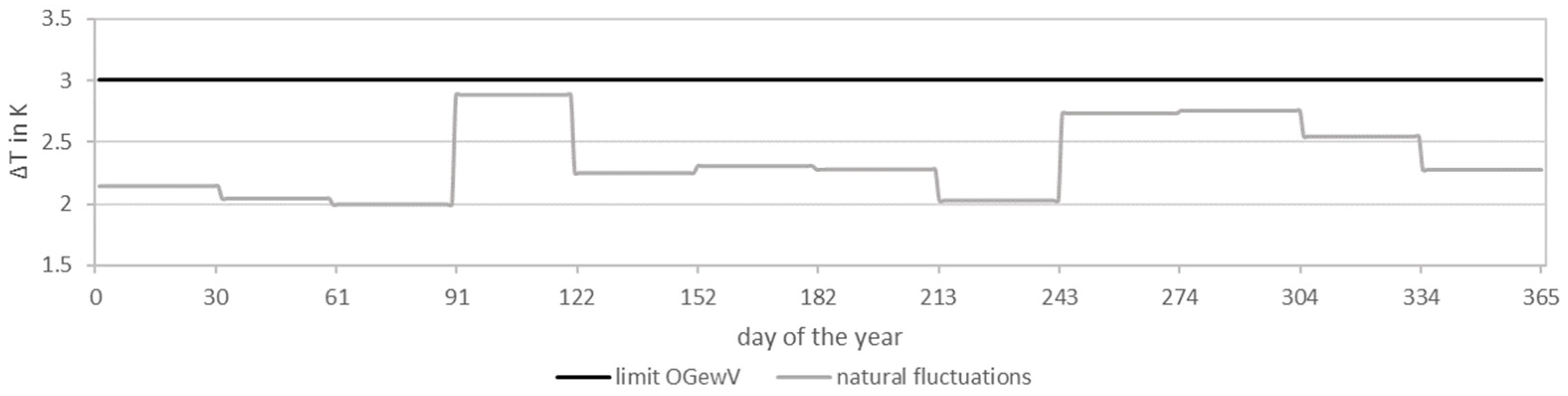
  • In Germany, the Regulation of Surface Waters (Oberflächengewässerverordnung, OGewV) sets limits for warming in water bodies, depending on the fish region, in order to ensure good water body status (see Table 6). To estimate a maximum temperature reduction, the maximum temperature increase prescribed in the OGewV can be assumed as the difference for cooling. As temperature increases are considered to be ecologically more serious than temperature decreases, the approach is considered justifiable at this point and is recommended by the Deggendorf Water Management Office [10], among others. To determine the river heat potential for district heating, a study by the IÖW assumed a general temperature change of 1 K [9], possibly to avoid uncertainties in the large-scale potential assessment.
Alternative approaches move away from blanket limit values and instead focus on the natural fluctuations in water temperatures or the warming trends caused by climate change. With global warming, temperatures in water bodies are also rising on average. This trend can be mitigated by the hydrothermal use of the water bodies. If the effects of climate change on water bodies can be quantified, then the permissible cooling of water bodies can be aligned with the temperature increase caused by climate change. A brief overview of the climate trend has already been provided (see Section 3.1.1); the following applies to the KLIWA regions and also to Marburg. Measurement data are currently being collected as part of a KLIWA study, but the scope and evaluation status of these data are not yet sufficient to make reliable statements on long-term effects caused by climate change [25]. It is also possible to limit the cooling to the natural fluctuations of the water [26]. For the natural fluctuations, the standard deviation or the confidence interval between the 15th and 85th percentile can be used as the average deviation from the long-term mean value (e.g., per day of the year).
Limit values are shown regardless of whether the minimum temperature for heat extraction is maintained in the water.
In Marburg, standard deviation is used for restriction to the natural fluctuations. Restricting the temperature change to natural fluctuations is the stricter approach here compared to the orientation of the OGewV (see Figure 13). This approach follows the recommendations of the GSchV to select stricter limit values with regard to the naturalness of temperature conditions, water quality, and self-purification capacity. One advantage of this restriction is the mild reduction in water temperature. Even if the climate trend is countered by cooling, the moderate change allows the ecosystem to acclimatize gently to this change. At locations with significant temperature increases due to heat input, a greater reduction in temperature may be more compatible with the ecology. This must be examined on a site-specific basis.
Limit values with regard to ecological compatibility refer to the difference between the unaffected water temperature and the mixing temperature. In order to mitigate local influences by temperature flags, individual restrictions have so far been set. In Germany, the responsible approval authorities decide on the extent of local temperature changes. These decisions have a direct impact on the maximum utilized heat potential. A maximum temperature change of 5 K for the extracted volume flow was specified in the approval notice by the approval authority for the Lauterecken local heat network [3] and for the IÖW district heating study [9]. The AGFW states a minimum cooling of 3 K in order to ensure economic efficiency [27].
In addition to ecological considerations, the technical and economic implementation of the system must also be taken into account. According to [1], the economic operation of the heat pump system is no longer guaranteed if the temperature falls below 4 °C. Lower temperatures are technically possible. In this case, there is a risk of ice forming on the system’s components. Various studies assume cooling to a minimum temperature of 1 °C [11], 2 °C [3,8,11], 3 °C [9,24], and 4 °C [27]. Overall, there is a trade-off between more days below the minimum temperature at high minimum temperatures (more challenging in terms of sufficient supply) and larger volume flows at low minimum temperatures (economically more critical) [11]. The demand for electrical heat pump power is also higher at low minimum temperatures.

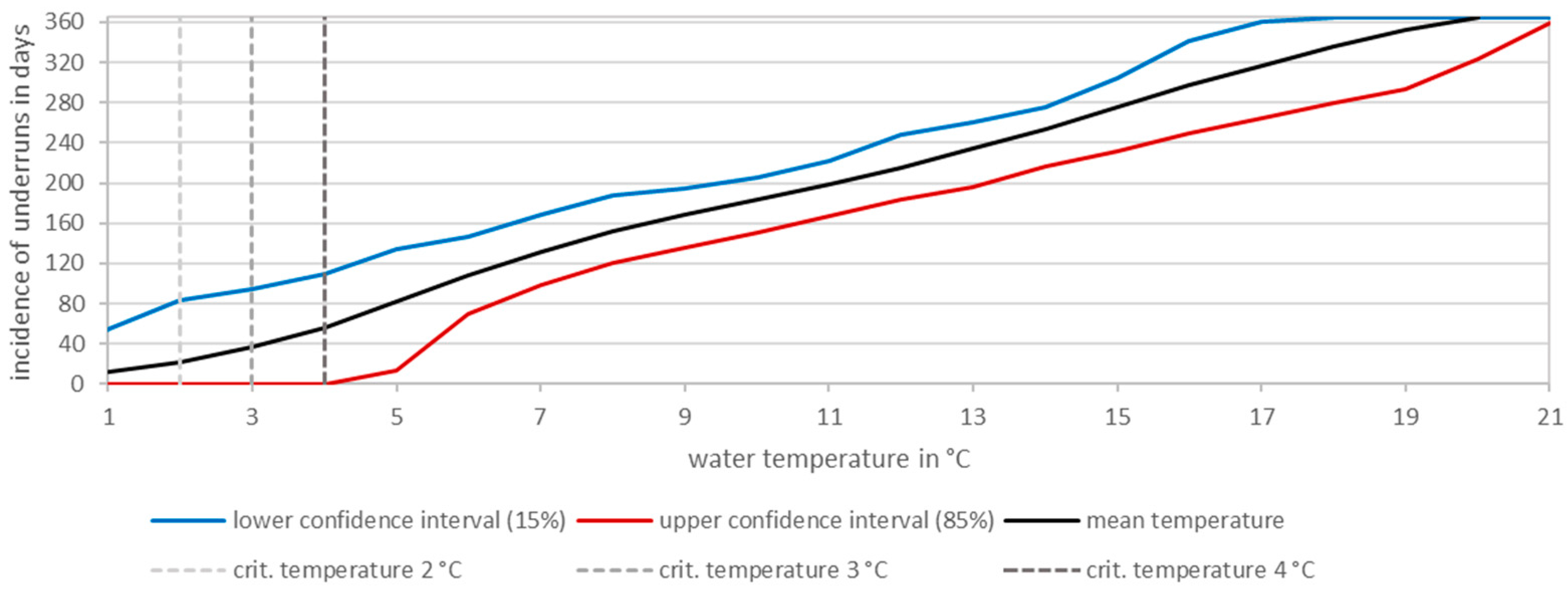
3.1.4. Analysis Parameters: Underrun Days

The selected critical temperature in the water, up to which the hydrothermal heat pump system is to be operated, influences both the economic efficiency of the system, because low critical temperatures mean higher volume flows and electrical heat pump power, and the supply stability, because the higher the critical temperature is set, the more frequently it is underrun and heat supply via river heat is no longer possible. Therefore, it is necessary to check whether the heat extraction rate compensates for the electrical power used under the specific conditions.
If heat demand cannot be covered by river heat alone due to water temperatures that are too low, due to very high supply temperatures or due to the provision of high peak outputs, a bivalent heat supply should be used. In order to have an overview of the effects of the choice of critical temperature on the number of underrun days, the incidence of underruns of the individual temperature values can be shown in the form of a duration curve (see Figure 14 for case study). It is not sufficient to evaluate the typical year based on monthly averages, as was performed, for example, to determine the renewable energy self-sufficient rate [28]. This is because the monthly average value does not imply anything about how many days (in a row) in a month the heat pump cannot be operated, which can become critical without heat storage. Instead, daily values are required, meaning both mean values and values in the lower confidence interval.
Table 7 shows the proportion of the heating period during which the heat demand must be covered by an alternative source or a purely electrically driven heat pump. Whether it is more economical to set a low critical temperature, to implement a bivalent operation by setting a higher critical temperature, or to use a heat storage tank must be examined individually. Germany is located in a moderately cool climate zone in the transitional area between the maritime climate of Western Europe and the continental climate of Eastern Europe. While the northern part of North Rhine-Westphalia is still more strongly influenced by the Atlantic, with rainy and mild winters, the continental influence is increased to the south. Marburg is close to the continental south of North Rhine-Westphalia, which is characterized by cold winters and low precipitation [29].
A closed heat extraction system is recommended because the temperatures fall below the critical temperatures. In practice, the temperature difference between the river water and the heat transfer medium (water hardness) is between 4 K and 6 K at the inlet [30]. This is intended to achieve a temperature spread of 3 K to 5 K in the heat transfer medium circuit [31]. If heat is to be extracted from the water even at temperatures at the freezing point, the heat transfer medium itself must already be frost-resistant (e.g., carbon dioxide) or be mixed with an antifreeze agent (e.g., ethylene glycol). In Germany, it is advisable to decide on the heat transfer medium and the implementation of the corresponding heat exchanger in close consultation with the approval authorities.

3.1.5. Analysis Parameters: Hydrothermal Coverage

If the correlation between water and air temperature is known, then future water temperatures can be derived on the basis of projected air temperature data. The IPCC produces international climate forecasts and climate projections at an international level, while the German Weather Service (Deutscher Wetterdienst, DWD, Offenbach, Germany) focuses on Germany. As the climate represents the long-term average state of weather conditions and the weather describes the current state of the atmosphere [32], forecasts for air temperature are more frequently available than those for water temperature. Local correlations between water and air temperatures also make it possible to estimate future water temperatures. In addition, an average annual profile of heat consumption can be created using the heating limit temperature and air temperature data, which are particularly informative in conjunction with the water temperature curve.
Figure 15 compares the water temperature with the annual profile of the contribution of heat consumption (space heating) according to VDI 3807-1. The contribution refers to the air temperatures in Marburg. There is an incoherence between heat supply and heat demand. While the water temperatures are high in summer and low in winter, the heat consumption is conversely high, especially in winter, but low or partially non-existent in summer. In rivers, the lower temperature values in winter are partially compensated for by higher flow rates (see Section 3.2). However, this effect does not occur if the discharge is regulated, as it is in the case of draining off the water. If, for example, a heat network with storage options and various supply points is operated, then the discrepancy can be reduced. In view of this discrepancy, it is important to determine the hydrothermal coverage ratio for different time periods and load types (base load, peak load) in order to select the appropriate operating mode (monovalent, monoenergetic, or bivalent).

3.1.6. Preliminary Considerations: Thermal Efficiency

The increased use of renewable heat sources plays a decisive role in reducing the use of fossil fuels and achieving global climate targets. Heat pumps are of great importance here, as they make environmental heat usable. Most environmental heat sources cannot be utilized everywhere or only on a limited scale. In addition to availability, the efficiency of the environmental heat source is also decisive in determining whether the source can be used economically. The thermal efficiency of the heat supply depends on the temperature difference between the heat sink and the heat source. The comparison of different heat sources is independent of efforts to reduce the supply temperatures on the heat sink side. This means that the guaranteed temperature level of the environmental heat source determines the efficiency of the heating system. Average temperatures that occur per environmental heat source are shown in Figure 16 and serve as an overview. Site-specific value ranges must be considered individually.

3.1.7. Analysis Parameters: Performance Factors (COP, SPF, SCOP)

The coefficient of performance COP and the seasonal performance factor SPF are interesting for quantifying the efficiency of heat sources. The COP indicates the ratio between the useful heat output and the electrical power; thus, it measures the current efficiency of the heat pump:
C O P = Q ˙ u s e P e l = η · T s i n k T s i n k T s o u r c e
  • C O P : Coefficient of performance;
  • Q ˙ u s e : Useful heat output in W;
  • P e l : Electrical power of heat pump in W;
  • η : Grade for heat source;
  • T s i n k : Temperature of heat sink in K;
  • T s o u r c e : Temperature of heat source in K.
The COP takes into account losses due to auxiliary drives from the heat source to the heating distribution system. The losses vary with the heat source (see Table 8). For each heat exchanger, a heat loss of 1 K can be added to Tsink [2]. The COP calculations for the Lahn river in Marburg were carried out for supply temperatures from Table 9. Supply temperatures of up to 70 °C should still be possible in the context of hydrothermal energy [11].
For a supply temperature of 55 °C, Figure 17 shows that the values over the entire year are between 3.0 and 4.6, with an average of 3.7 ± 0.7. During the heating period, the values are between 3.2 and 3.8, with an average of 3.4 ± 0.4. The comparison shows that the COP values above 4.0 occur exclusively outside the heating period.
The comparative analysis of the COP values for different supply temperatures (45 °C, 55 °C and 65 °C) shows that the COP values increase as the supply temperature decreases (see Figure 18). The frequency of the COP values generally decreases as the COP value increases. As the heat supply is particularly relevant during the heating period, only values from the heating period were used for the comparative analysis.
With otherwise constant variables, the COP depends solely on the water temperature and, like the water temperature in the hydrograph, showed a sinusoidal curve over the year (see Figure 19). While the COP reached its peak in the middle of the year (COP55,max = 4.5), it had its lowest values (COP55,min = 3.2) in the cold months of December to February. Regarding the contribution of heat consumption (space heating), it was noticeable that the high COP values can hardly be utilized in summer, as no space heating is required during this period, while heat consumption is high in the heating period and the COP values are low. In order to take the proportionate heat consumption into account, the COP was weighted and averaged. It was 3.4 for the provision of space heating and 3.5 for the combined provision of space heating and hot water. The weighted COP was slightly higher with the provision of hot water, as hot water is also required in the summer; therefore, high COP values in summer were taken into account.
While the COP indicates the current efficiency of a heat pump, the seasonal performance factor SPF examines the efficiency of the heat pump over the entire year and takes into account the energy used in relation to the heat generated. It is used to compare the efficiency of heat pump systems. The SPF is determined under real conditions and depends on various factors, such as the operating mode and ventilation habits. It can only be determined after a heating system has been commissioned. In the planning phase, a calculated seasonal coefficient of performance (SCOP) can be determined based on standardized boundary conditions (according to German VDI Guideline 4650, Sheet 1) [34]. The guideline does not explicitly list surface water as a heat source. The calculation rule for groundwater comes closest to it. For Marburg, the SCOP is 3.7 (correction values FΔϑ = 1.0, Fϑ = 0.902, and FP = 1.035; standardized COPN = 4.3).
As several studies [35,36,37,38] have compiled the seasonal performance factors of heat pump systems, the determination of the SPF or SCOP for the planned hydrothermal system is a good way of comparing the calculated performance. However, since the seasonal performance factor not only takes into account the heat source but is also influenced by the usage behavior and the insulation properties of the heat sink, comparability is limited. A careful analysis of the COP is therefore recommended. The average COP values for the heating period and the weighted COP values are more meaningful for assessing efficiency than the SPF values. The weighted COP values are more meaningful than the average values for the heating period. The following applies to Marburg: as the value deviations between the two methods are not large (ΔCOPm,45 °C = 0.1; ΔCOPm,55 °C = 0; ΔCOPm,65 °C = 0), averaging the values from the heating period is sufficient here for reasons of practicability.

3.2. Discharge (Macroscopic)

Flow measurement data are crucial for calculating the permissible heat potential. Equation (1) shows that both the temperature and the discharge determine how much heat can be extracted. While temperatures in moderate climate zones are on average lower in winter than in summer, the average discharge in pluvial rivers is higher in winter than in summer. To ensure that the calculations of the heat potential not only refer to the area of the measuring level (flow) but also apply to the corresponding site, there should be no water inflows or outflows between the site and the level used for the flow values. If water from a bypass is used for heating purposes, then not all of the water body’s heat can be utilized. The maximum utilized heat potential is therefore limited by the discharge in the bypass. The possible heat extraction rates depend on the discharge as follows:
  • Open heat extraction system: Up to 20% of the discharge can be extracted from the water body by means of suction extraction [39]. For higher extraction rates, separate extraction structures in the form of side, front, or bottom extraction make sense.
  • Closed heat extraction system: If the geometric conditions and water depths are known, then the discharge can be used to determine the flow velocity, which influences the efficiency of the closed heat extraction system and biofilm formation.
The flow data also provide information on whether there is sufficient cover for the suction pipe (open system) or the heat exchanger (closed system) in the event of low water.
For this case study, the time series of RAPS for the discharge values over time showed a trend with several smaller irregularities (see Figure 20). The parabolic shape of the RAPS values indicates a continuous unidirectional discharge trend. As described in Section 3.1.1, the trend can be caused, for example, by a gradually changing environment, like one affected by climate change [17]. Here, discharges decreased over time. An irregularity can be found from 1994 to 1997.
For this case study, the characteristic course of the discharge is shown via a hydrograph (see Figure 21). The flow is highest at the beginning of the year and shows a pluvial discharge regime according to [40]. For the heat potential, the lower temperature values in winter can be partially compensated for by the higher discharge in winter. The values flatten out towards summer and are at their lowest from around July to September. In summer, the confidence interval is narrow, which indicates a constant discharge compared to the rest of the year. Thereafter, the discharge increases again, and the confidence interval widens. The effects of the flow rates on the flow velocities depend on local conditions, such as bed gradient and bed roughness, and must be examined on a site-specific basis. The water depth varies locally with the cross-section geometry and the flow velocity.

3.3. Water Depth (Vertical)

Water depth is of great importance when using rivers for hydrothermal purposes. This is because the river as a heat source is only available when the water body has sufficient water to ensure that the heat exchanger (closed system) or the extraction pipe (open system) is covered. If the discharge and profile of the cross-section are known, then the water depth can provide information about the flow velocity, which influences the efficiency of the closed heat extraction system and biofilm formation.
Little literary research gives information about the design parameters of suction pipes, which set the required minimum water depth. To prevent the bed substrate from being stirred up, the inlet opening of the suction pipe must be positioned at least 0.6 m as per [41] or two to four pipe diameters as per [42] above the water bed. The safety distance to the water surface against ice effects and water level fluctuations is at least 0.4 m [41]. The safety distance to the water surface can be adopted for heat exchangers. The distance to the water bed can be less, as the heat exchanger does not generate a suction effect that can stir up the bed substrate. Depending on the design of the heat exchanger, a safety distance is nevertheless recommended in order to reduce contamination of the apparatus by the bed substrate. A minimum cover of the suction pipe is also necessary in order to avoid air-drawing vortices. Corresponding calculation approaches can be found in the literature, e.g., [43]. It is also recommended to install an anti-vortex plate above the suction strainer located at the inlet to the suction pipe [41,44]. Overall, a 0.9 m minimum water depth is suggested as per [44]. With the selected diameter of the suction pipe or the selected height of the heat exchanger and the safety distances to the water surface and the bottom as per [41], this results in the following minimum water depth for hydrothermal use:
h m i n = Δ h w s + h h e s + Δ h b e d = m a x 0.4 ; Δ h v o r t + d p i p e + 0.6     ,   o p e n   s y s t e m 0.4 + h h e + Δ h b e d , h e     ,   c l o s e d   s y s t e m
  • h m i n : Minimum water depth in river in m;
  • Δ h w s : Distance to water surface in m;
  • h h e s : Height of heat extraction system in m;
  • Δ h S o : Distance to river bed in m;
  • Δ h v o r t : Distance because of air-drawing vortices in m;
  • d p i p e : Diameter of the suction pipe in m;
  • h h e : Height of heat exchanger in m;
  • Δ h b e d , h e : Distance to river bed in m, heat exchanger specific.
Water depths are not available for every site. The water depths in millraces may be recorded by the plant operator himself. If measured values for discharge and information on the profile of the cross-section and wall roughness are available, then the water depth can be estimated using the Gauckler–Manning–Strickler flow formula. Otherwise, measurements will need to be taken, at least on a sample basis.
As a site-specific parameter, the water depth for this case study was considered at site 1 (Wehrda waterworks). In order to calculate water depths from the known measured data on the water level above sea level, the smallest measured value of the water level was assumed as the river bed level above sea level. The water depths in a typical year range between 0.7 m ± 0.1 m (middle of the year) and 1.3 m ± 0.5 m (turn of the year) (see Figure 22). If a diameter of at least 12.5 cm is selected for the suction pipe (open heat extraction system) in accordance with [41], this results in a minimum water depth of 1.125 m, including safety distances. The minimum water depth was reached on an average of 76 days (21% of the days in the year). The lower water depths of the confidence interval did not reach the minimum water depth in the entire characteristic year. In order to enable the implementation of a hydrothermal system at this site, the following should be examined in detail:
  • How an increase in water depths could be achieved (e.g., via ground sills);
  • Whether bank filtration should be installed;
  • Whether the safety distances can be reduced.

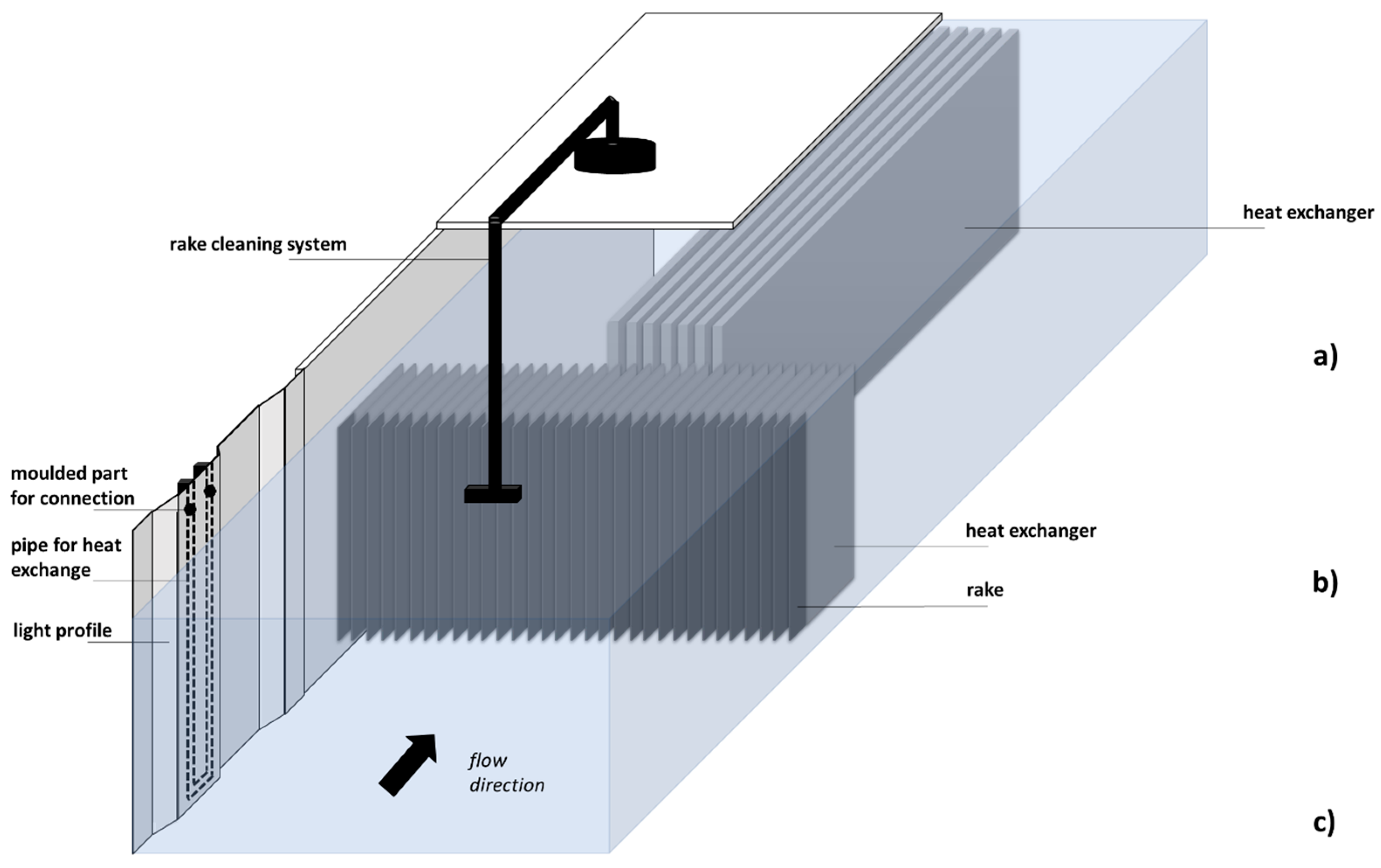
3.4. River Geometry (Horizontal)

In addition to water depth (vertical dimension), horizontal dimensions also play an important role in the implementation of heat extraction. There must be sufficient space for the installation of the system and minimum distances to other uses. The minimum distances can be particularly relevant for open heat extraction systems in order to take into account the suction effect of the suction extraction and the jet effect of the reintroduction. In Germany, the approval authorities are responsible for determining the distances to shipping.
The amount of space required depends largely on whether the water heat is extracted via an open or closed system. Suction pipes generally require less space than heat exchangers, as a large part of the system technology is installed outside the water. If no intermediate heat exchanger is required before the heat pump, then water extraction also has the advantage that lower heat losses occur and that water acts as a heat transfer medium and, therefore, has a higher heat storage capacity than a frost protection-based heat transfer medium in the heat exchanger. The space required in the water is also influenced by the heat requirement. It determines the diameter of the suction pipe or the surface area of the heat exchanger. The design of the heat exchanger can be adapted to different water geometry requirements (see Figure 23). Free-standing units (a) are usually long and narrow. Thermal rakes (b) are heat exchangers on the rack of a hydropower plant and take up a lot of space in width but not in length. In the case of energy sheet pile walls (c), the principle of thermo-active concrete components is transferred to steel sheet pile walls. They consist of sheet piles that are equipped with additional absorber tubes for heat extraction. Sheet piling is mainly used where groundwater is present and is, therefore, usually located in energetically favorable subsoil. In the area of port or hydraulic engineering, direct contact with the surface water is guaranteed. The energy sheet pile walls utilize the existing infrastructure, which means that only a small amount of additional space is used near the wall.
Near-bottom units, such as horizontal collectors (see Figure 24), can offer an alternative if the water depth is insufficient. Originally designed for near-surface geothermal energy, they are laid out on the ground and are particularly suitable for shallow and long stretches of water. Sediment collectors (a) can be laid either straight or in loops. With spiral collectors (b), the loops are wound into pipe bundles. In this case, a pipe spacing must be maintained that ensures the flow around the individual pipes protruding into the flow. The individual tube bundles have lengths of 100 m to 150 m and are arranged one behind the other with a minimum spacing of 6 m [31]. Flat spiral coils (c) can be suitable for locations with low elongation. Slinky coils (d) are characterized by winding over the length with a high pipe density.

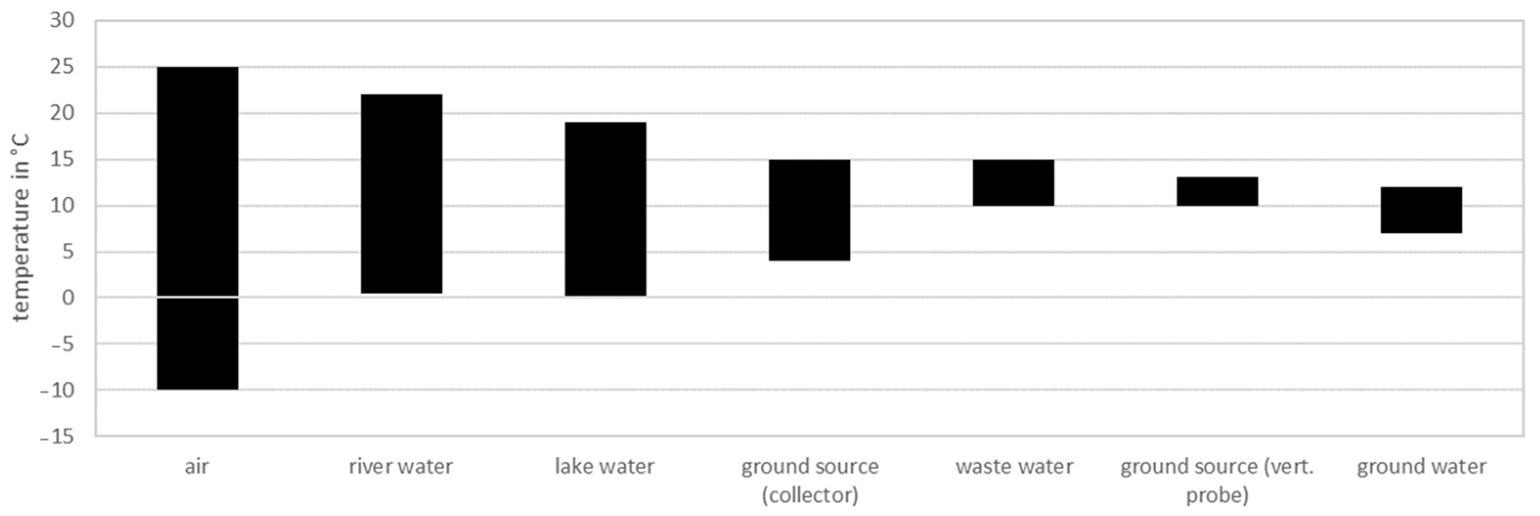
3.5. Distance to the Connection, Ground Temperature

The length of the transport pipes influences the economic efficiency of the individual operational areas. The following factors play a role here:
  • Thermal efficiency (heat losses or gains in the pipes);
  • Electricity costs (pressure losses in the pipes);
  • Material costs (pipes, insulation material if necessary);
  • Construction costs (laying the pipes).
Electricity costs, material costs, and construction costs generally increase with the length of the pipe. Thermal efficiency and material costs are also influenced by ground temperatures. A comparison of ground and water temperatures helps to assess whether heat is transferred from the ground into the pipes or whether water heat is transferred from the pipes into the ground. In order to estimate the ground temperatures in Marburg, the three nearest stations around Marburg were analyzed (see Figure 6). Measured values were available for soil depths of 5 cm, 10 cm, 20 cm, and 50 cm. Measurement data below the frost line, which is around 80 cm in Central Europe, were not available. The greatest soil depths of 20 cm and 50 cm were considered further. Over the course of the year, a sinusoidal curve can be seen with a high point in July and August and a low point in January and February (see Figure 25). While the 20 cm curve shows fluctuations influenced by the weather, the 50 cm curve is more moderate. One reason for this is the decreasing influence of air temperature and solar radiation on ground temperature with increasing depth.
The following applies to the average values from the three measuring stations (see Figure 26) at a depth of 20 cm: Between November and March, the ground temperatures are lower than the water temperatures. During the majority of the heating period, heat is therefore dissipated via the transport pipes. Shorter pipe runs are therefore recommended. In the mild to warm months, the ground serves as an additional heat source. For the ground at a depth of 50 cm, an attenuation and shift in temperature differences can be observed. In the first half of the year, heat can be expected to escape from the pipes, and in the second half of the year, heat can be expected to enter the pipes. With the use of heat storage technologies, the ground can represent an additional heat source in the annual total so that longer pipe runs can be advantageous in terms of heat energy. The sum of the temperature differences is positive in the typical year (150 K∙d in 20 cm, 140 K∙d in 50 cm).
Analogous to water extraction, a comparison of ground temperature with the temperature of the used water is also important. A critical case occurs when heat is extracted close to the surface and the ground is cold. This is because it must be ensured that the water temperatures in the return flow are not so strongly influenced by the ground temperatures that the permissible temperature change on return to the water body is overstimulated. If heat is extracted when the ground is warm, then there is an opportunity to partially compensate for the heat extraction from the water by the geothermal heat input in the return flow so that greater heat extraction is possible.

3.6. Existing Infrastructure

In addition to the characteristics of the water body, hydrothermal-positive characteristics of the surroundings are also relevant. In terms of infrastructure, spatial, electrical, and thermal integrations play a role (see Figure 27). Spatial integration: To transport the heat from the river to the heat pump and from the heat pump to the heat sinks, sufficient space must be available for the pipes. If existing pipelines can be used or construction work is planned, then costs for the pipes can be reduced. A new waterworks is to be built at the Wehrda waterworks in Marburg. Here, the simultaneous installation of a pipe infrastructure for a future hydrothermal system is a suitable option. Furthermore, sufficient space must be available for the heat pump system. This can be particularly difficult in city centers [47]. In Wehrda, for example, the pump house of the old waterworks can be used to install an intermediate heat exchanger. Electrical integration: To operate a heat pump, it must be connected to a sufficiently strong power grid. Up to seven times more electricity may be required to start a heat pump than for normal operation [47]. Thermal integration: The integration of the river heat into the heat sinks, e.g., through a heat network, is necessary, and suitable supply temperatures are also important (see Section 3.1.7).

3.7. Flow Velocity, Turbulence

It is not only relevant how much water flows per time (discharge) but also how the water flow is characterized (flow velocity, turbulence). Turbulence influences the mixing of the used water with its surroundings and, thus, the length of the temperature flag behind the extraction point. A temperature flag can be described as water with a difference of at least 1 K to the surrounding water [48]. The flow velocity influences both thermo-fluid dynamic processes and deposition processes at the heat exchanger. A minimum flow velocity of 0.3 m/s at the heat exchanger prevents the deposition of suspended solids and reduces biofilm formation [12]. Up to 0.4 m/s, the increase in heat transfer with increasing velocity is large [12]. In the open heat extraction system, a higher flow velocity can reduce the formation of a submersible funnel on the suction pipe.

3.8. Water Quality

Suspended solids and organic matter in the river contaminate the heat source system. The resulting fouling and silting of the heat exchanger reduce heat transfer. In open systems, filters are used for the water extraction structure. A balance must be struck between protecting the system components from suspended solids (small filter mesh size) and minimizing pressure losses and cleaning intervals (large filter mesh size). The cleaning frequency increases as the proportion of suspended solids and organic matter increases. When extracting water, it is also recommended to purify the extracted water via sedimentation tanks or ball filters before heat extraction. As qualitative information on the proportion of suspended solids and organic matter is rarely available, a qualitative assessment can be performed by means of a visual sample, for example. For Marburg, a qualitative inventory analysis is available from HLNUG.

3.9. Balancing of Alternatives

With the switch from fossil fuels to renewable energy sources, environmental heat sources in particular will come into focus in the future instead of coal. Due to their thermal regeneration capability and the high specific heat capacity of water, surface waters are very well suited as an environmental heat source. Most environmental heat sources cannot be used everywhere or can only be used to a limited extent. Geothermal systems require sufficient open space and suitable soil conditions; for biomass, the availability of raw materials is a limitation; the economic viability of aerothermal energy is questionable, especially beyond the scale of a residential unit. Therefore, hydrothermal energy represents a great opportunity not only for private owners but especially for public utilities. When considering whether a potentially expensive and innovative hydrothermal system is worthwhile, it is also important to examine which alternative supply systems are even worth considering and what their monetary and climatic impact would be.

3.10. Heat Potential and Heat Demand

Equation (1) for calculating the heat potential gives rise to challenges in determining the individual physical variables. Various studies use different values for the discharge, e.g., the mean discharge per month or quarter [2], the minimum daily mean over 77 years per month [8], the low water discharge [10], or a sensitivity-specific proportion of the winter discharge as a constant value over the year [7]. In this paper, a hydrograph was used over the typical year, with daily mean values and confidence intervals. The mean low water discharge (per heating period or year) was used for dimensioning. Hereafter, an average scenario with average flow values and a discharge-critical scenario with flow values in the lower confidence interval were considered. The water temperatures were treated equivalently.
Cooling must be kept within the natural fluctuations. Temperatures between 1 °C and 4 °C can be found in the literature, up to which the water can be used thermally. In this case study, the potential curves for 2 °C and 3 °C critical temperature coincided. While the heating period can practically not be used at a critical temperature of 4 °C, hydrothermal use is almost always possible at a critical temperature of 3 °C (see Figure 28). In the scenarios for cooling to a minimum temperature, the 0 °C curve coincided with the 1 °C curve, as the natural fluctuations usually limit the permissible cooling to up to 2 K during the heating period. In the following, a critical temperature of 3 °C and a minimum temperature of 1 °C are assumed.
The comparison of scenarios with different probabilities of occurrence (see Figure 29) showed that the heat potential for average discharges and temperatures in the lower confidence range is just as high as in the medium scenario, apart from the days of the year on which the temperatures fall below the critical temperature. Here, the heat potential corresponded to zero. With medium temperatures and discharges in the lower confidence interval, all days of the year could be used, but the heat potential was generally lower. In concrete terms, this means that the discharge in particular influences the size of the heat potential, while the water temperature determines whether and how thermal utilization is possible. With this in mind, it makes sense to compare heat consumption not only with water temperature (see Section 3.1.7) but also with the discharge. Figure 30 shows that the discharge as a value that determines the size of the heat potential is coherent with the heat consumption (correlation coefficient R = 0.78).
The temperature dependence of the specific heat capacity and density of water had only a slight effect on the heat potential (see Figure 31). The deviation between the two curves was up to 0.5% of the constant potential. The potential varied by up to 700 kW, which could supply several households with heat but was insignificant in view of the overall potential.
According to Equation (1), the heat potential is proportional to the discharge. This means that once the total heat potential has been calculated, it can be quickly adapted to the conditions at the specific site. For example, if one third of the incoming water flows through a millrace, one third of the previously calculated heat can be extracted from it.
The calculated heat potential of the Lahn river in Marburg is compared in Table 10 with the heat potentials from potential analyses presented in Section 1. With similar discharges, the heat potential is also in the same order of magnitude.
In order to determine the maximum hydrothermal coverage per day, the heat demand must be compared with the heat output of the heat pump in the medium scenario. The heat demand is based on the previous heat consumption but can also take consumption forecasts into account where feasible. For the heat output of the heat pump, the heat potential of the Lahn river is combined with the day-specific COP. The shares can then be averaged per month or per heating period and complementary period. For a realistic estimate of the hydrothermal coverage, the usable discharge share of the MNQ must be estimated. As the COP is low, particularly in the heating period, due to the low water temperatures (see Section 3.1.7), the cost-effectiveness and efficiency of the system can be improved by not operating it monovalently but by using the hydrothermal energy to cover the base load. The base load covers up to 80% of the total annual work and amounts to between 10% and 40% of the maximum output [49]. Base load modules can be defined above a relative plateau within this range, or the standard approaches of public utilities can be used. There are also research approaches for developing an economically and ecologically optimized design method [50]. In this context, hydrothermal coverage is the proportion of days heated with hydrothermal energy out of the total heating days per year.
In the annual duration curve of the Stadtwerke Marburg (see Figure 32), the base load modules A and B were each assumed to be above a relative plateau in the base load range. The base load A was 210 kW (14% of the peak load, exceeded on 7100 h), means 20% hydrothermal coverage and could be covered with a COP = 2 via 2 DN125 suction pipes (4.5 K spread, of which 1 K heat loss). The base load B was 325 kW (21% of the peak load, exceeded on 5359 h), means 40% hydrothermal coverage and could be covered with a COP = 2 via 3 DN125 suction pipes (4.5 K spread, of which 1 K heat loss).

4. Conclusions and Discussion

Heat pumps enable the use of environmental heat and thus help to shift the supply of heat away from fossil fuels. Due to the high specific heat capacity of water and natural thermal regeneration, rivers are an interesting environmental heat source. How much heat rivers can provide (potential analysis) can be determined quantitatively via the permissible heat potential. For this purpose, the two macroscopic influencing factors of water temperature and discharge must be analyzed. The basis is the representation of the daily measured values via hydrographs for a typical year. The water temperature must be evaluated in relation to underrun days (duration curve) and performance figures (weighted). In order to determine the heat potential, critical values for the temperature change must also be defined. It should be noted that the discharge in particular influences the size of the heat potential, while the water temperature determines whether and how thermal utilization is possible. In addition, other influencing factors are decisive for the question of whether hydrothermal utilization makes sense at specific sites (feasibility study). Table 1 proposes the relevant influencing factors. Legal requirements must be complied with. In addition, the water depths are decisive for whether the site can be used hydrothermally. This is because both the suction pipe and the heat exchanger must be sufficiently covered in order to use the river water. The distance to the heat connection and the water quality are also relevant. They determine whether the use can be economical at all. How profitable hydrothermal energy can be ultimately depends on the water geometry, the flow velocity and turbulence, the existing infrastructure, and the possible supply alternatives. Unfortunately, not all information is available, or measured values are available. In some cases, it is possible to work with sample data or estimates. Sometimes, simplifications are helpful, such as for water depth. Channels that are already anthropogenically influenced are suitable for hydrothermal use. These usually have a rectangular channel. In this case, the water depth at each point is approximately the mean water depth. This simplification was made in this paper because the sites in the case study have rectangular channels. If a natural body of water is to be used, then water depth must be considered at the exact point where the heat extraction system is to be installed. The same applies to the horizontal dimensions, flow velocity, and turbulence. At the site under consideration, it must be checked whether such simplifications can be made, whether information about the precise extraction point is available, or whether measurements must be taken at the exact extraction point. In general, it can be stated that the more information is known, the more meaningful the analysis can be.

Author Contributions

Conceptualization, J.G.; methodology, J.G. and S.B.; validation, S.B. and B.L.; formal analysis, J.G.; writing—original draft preparation, J.G.; review and editing, S.B. and B.L.; visualization, J.G. All authors have read and agreed to the published version of the manuscript.

Funding

This research received no external funding. The Article Processing Charges (APC) were funded by the Deutsche Forschungsgemeinschaft (DFG, German Research Foundation) and the Open Access Publishing Fund of the Technical University of Darmstadt.

Data Availability Statement

Mostly, publicly available datasets were analyzed in this study. To find these data, see Table 2 in this paper. Restrictions apply to the availability of heat consumption data and water temperature data at the Wehrda waterworks. These data were obtained from Stadtwerke Marburg GmbH and are available from the public utilities with their permission.

Acknowledgments

The corresponding author acknowledges the financial support by the Deutsche Forschungsgemeinschaft (DFG, German Research Foundation) and the Open Access Publishing Fund of the Technical University of Darmstadt for the Article Processing Charges (APC) and says thank you to her team in the chair of Hydraulic Engineering for the support in any aspect.

Conflicts of Interest

The authors declare no conflict of interest.

References

  1. Marotz, G. Der Einsatz von Wärmepumpen in fließenden Gewässern—Wasserwirtschaftliche und betriebliche Aspekte. Wasserwirtschaft 1977, 67, 376–381. [Google Scholar]
  2. Gaudard, A.; Schmid, M.; Wüest, A. Thermische Nutzung von Seen und Flüssen: Potenzial der Schweizer Oberflächengewässer. Aqua Gas 2018, 2, 26–33. [Google Scholar]
  3. Schwinghammer, F. Thermische Nutzung von Oberflächengewässern. Master’s Thesis, Albert-Ludwigs-Universität Freiburg, Freiburg, Germany, 2012. [Google Scholar]
  4. Borchardt, S. Wärmetechnische Nutzung von Fließgewässern. J. Arbeitsschutz Umw. 2018, 1, 21–24. [Google Scholar]
  5. Schmid, M.; Gaudard, A. Potenzial des Walensees für Wärme- und Kältenutzung; Amt für Wasser und Energie des Kantons St. Gallen: St. Gallen, Switzerland, 2019. [Google Scholar]
  6. Gaudard, A. Wärme- und Kältenutzung aus Brienzer-, Thuner- und Bielersee: Abschätzung des Potenzials und Beeinflussung der Seeökosysteme; Eawag: Kastanienbaum, Switzerland, 2016. [Google Scholar]
  7. Department of Energy & Climate Change. National Heat Map: Water Source Heat Map Layer; Department of Energy & Climate Change: London, UK, 2015. [Google Scholar]
  8. Anton, S. Thermische Nutzung Rhein: Schlussbericht Potentialstudie; Eichler + Pauli: Bern, Germany, 2016. [Google Scholar]
  9. Dunkelberg, E.; Deisböck, A.; Herrmann, B.; Hirschl, B.; Mitzinger, T.; Röder, J.; Salecki, S.; Thier, P.; Wassermann, T. Fernwärme Klimaneutral Transformieren: Eine Bewertung der Handlungsoptionen am Beispiel Berlin Nord-Neukölln; Schriftenreihe des Institut für Ökologische Wirtschaftsforschung 218/20; Institut für Ökologische Wirtschaftsforschung: Berlin, Germany, 2020. [Google Scholar]
  10. Wasserwirtschaftsamt Deggendorf. Wärmetauscher in Oberirdischen Gewässern: Wasserwirtschaftliche Betrachtung; Wasserwirtschaftsamt Deggendorf: Deggendorf, Germany, 2011. [Google Scholar]
  11. Gaudard, A.; Wüest, A.; Schmid, M. Using lakes and rivers for extraction and disposal of heat: Estimate of regional potentials. Renew. Energy 2019, 134, 330–342. [Google Scholar] [CrossRef]
  12. Marotz, G.W. Model Tests to Investigate Water-Circulation in Heat Pumps. In Proceedings of the 17th Congress of the International Association for Hydraulic Research, Baden-Baden, Germany, 14–19 August 1977; pp. 291–297. [Google Scholar]
  13. Maniak, U. Hydrologie und Wasserwirtschaft: Eine Einführung für Ingenieure, 7th ed.; Springer Vieweg: Berlin, Germany, 2016. [Google Scholar] [CrossRef]
  14. Deutsche Vereinigung für Wasserwirtschaft, Abwasser und Abfall e.V. (DVWK). Statistische Analyse von Hochwasserabflüssen. Merkblätter zur Wasserwirtschaft; Deutsche Vereinigung für Wasserwirtschaft, Abwasser und Abfall e.V. (DVWK): Hennef (Sieg), Germany, 1999. [Google Scholar]
  15. Linke, C. Leitlinien zur Interpretation Regionaler Klimamodelldaten des Bund-Länder-Fachgesprächs “Interpretation Regionaler Klimamodelldaten”; Landesamt für Umwelt Brandenburg: Potsdam, Germany, 2023. [Google Scholar]
  16. Kos, Z.; Durin, B.; Dogancic, D.; Kranjcic, N. Hydro-Energy Suitability of Rivers Regarding Their Hydrological and Hydrogeological Characteristics. Water 2021, 13, 1777. [Google Scholar] [CrossRef]
  17. Garbrecht, J.; Fernandez, G.P. Visualization of Trends and Fluctuations in Climatic Records. Wasser Resour. Bull. Am. Water Resour. Assoc. 1994, 30, 2. [Google Scholar]
  18. Caissie, D. The thermal regime of rivers: A review. Freshw. Biol. 2006, 51, 1389–1406. [Google Scholar] [CrossRef]
  19. van Vliet, M.; Franssen, W.; Yearsley, J.R.; Ludwig, F.; Haddeland, I.; Lettenmaier, D.P.; Kabat, P. Global river discharge and water temperature under climate change. Glob. Environ. Chang. 2013, 23, 450–464. [Google Scholar] [CrossRef]
  20. Orr, H.G.; Simpson, G.L.; Des Clers, S.; Watts, G.; Hughes, M.; Hannaford, J.; Dunbar, M.J.; Laizé, C.; Wilby, R.L.; Battarbee, R.W.; et al. Detecting changing river temperatures in England and Wales. Hydrol. Process. 2015, 29, 752–766. [Google Scholar] [CrossRef]
  21. European Environment Agency. Climate change, impacts and vulnerability in Europe 2016: An indicator-based report. Publications Office of the European Union. EEA Rep. 2017, 1. [Google Scholar] [CrossRef]
  22. Bay, O. Kalibrierung und Validierung Eines Wasserhaushalts- und Wärmemodells zur Simulation von Fließgewässertemperaturen. Master‘s Thesis, Technische Universität Darmstadt, Darmstadt, Germany, 2023. [Google Scholar] [CrossRef]
  23. Lange, J. Wärmelast Rhein: Studie; BUND: Mainz, Germany, 2009. [Google Scholar]
  24. WFD UK TAG. UK Environmental Standards and Conditions (Phase 2); UK Technical Advisory Group on the Water Framework Directive: Wallscope, Edingburgh, 2008. [Google Scholar]
  25. KLIWA. Klimawandel in Süddeutschland. Veränderungen von Meteorologischen und Hydrologischen Kenngrößen: Monitoringbericht 2021; Landesamt für Umwelt Rheinland-Pfalz: Mainz, Germany, 2021. [Google Scholar]
  26. Güttinger, H. Wärmepumpen an Oberflächengewässern: Ökologische Probleme und Einsatzmöglichkeiten in der Schweiz; Schriftenreihe des Bundesamtes für Energiewirtschaft: Bern, Switzerland, 1981. [Google Scholar]
  27. AGFW. Praxisleitfaden Großwärmepumpen; AGFW: Frankfurt, Germany, 2020. [Google Scholar]
  28. Kim, Y.; Yu, K.-H. Constructing a Database of Reference Hydrothermal Sources for a Zero-Energy Building Certification Rating in South Korea and Analyzing the Renewable Energy Self-Sufficiency Rate Achieved by Water-Source Heat Pumps. Energies 2023, 16, 543. [Google Scholar] [CrossRef]
  29. Ministerium für Umwelt, Landwirtschaft, Natur- und Verbraucherschutz des Landes Nordrhein-Westfalen (MULNV NRW). Bewirtschaftungsplan 2022–2027 für die Nordrhein-Westfälischen Anteile von Rhein, Weser, Ems und Maas; MULNV NRW: Düsseldorf, Germany, 2021. [Google Scholar]
  30. Kammer, H. Thermische Seewassernutzung in Deutschland: Bestandsanalyse, Potential und Hemmnisse Seewasserbetriebener Wärmepumpen; Springer Vieweg: Wiesbaden, Germany, 2017. [Google Scholar] [CrossRef]
  31. Koppmann, D. Untersuchung der Thermischen Aktivierung von Stahlspundwänden. Ph.D. Dissertation, Aachen University, Aachen, Germany, 2021. [Google Scholar]
  32. DWD. Wetter- und Klimalexikon, Klima. 2022. Available online: https://www.dwd.de/DE/service/lexikon/Functions/glossar.html?lv2=101334&lv3=101462 (accessed on 15 November 2023).
  33. Zogg, M. Zertifikatslehrgang ETH in Angewandten Erdwissenschaften: Geothermie—Die Energie des 21. Jahrhunderts; ETH Zürich: Oberburg, Switzerland, 2009. [Google Scholar]
  34. Verein Deutscher Ingenieure. Berechnung der Jahresarbeitszahl von Wärmepumpenanlagen: Elektrowärmepumpen zur Raumheizung und Trinkwassererwärmung; Beuth: Berlin, Germany, 2019. [Google Scholar]
  35. Ehrbar, M.P. Prüfungen im Testzentrum schaffen Vertrauen: Rückblick, Ausblick und Vergleich mit Feldbetrieb. In FAWA, Feldanalyse von Wärmepumpen-Anlagen; Rognon, F., Ed.; Bundesamt für Energie: Bern, Switzerland, 2004; pp. 27–38. [Google Scholar]
  36. ISE. Feldmessung Wärmepumpen im Gebäudebestand: Abschlussbericht; Fraunhofer Institut Solare Energiesysteme: Freiburg, Germany, 2010. [Google Scholar]
  37. Rognon, F. (Ed.) FAWA: Feldanalyse von Wärmepumpen-Anlagen; Bundesamt für Energie: Bern, Switzerland, 2004. [Google Scholar]
  38. BAFA. Wärmepumpe: Grundwissen zum Marktanreizprogramm; Bundesamt für Wirtschaft und Ausfuhrkontrolle: Eschborn, Germany, 2019. [Google Scholar]
  39. Scheuerlein, H. Die Wasserentnahme aus Geschiebeführenden Flüssen; Ernst Verlag: Berlin, Germany, 1984. [Google Scholar]
  40. Pardé, M. Fleuves et Riviéres; Colin: Paris, France, 1964. [Google Scholar]
  41. Deutsches Institut für Normung. Künstlich Angelegte Löschwasserteiche: Artificially Constructed Water Ponds for Fire Fighting; Beuth: Berlin, Germany, 2019; DIN 1420. [Google Scholar]
  42. Peterson, A.W.; Bouthillier, P.H.; Charbonneau, A.L.; Yaremko, E.K. River Intake Structures. In Pumping Station Design for the Practical Engineer: Water; Sank, R.L., Reh, C.W., Eds.; Montana State University: Bozeman, MT, USA, 1981. [Google Scholar]
  43. KSB SE & Co. KGaA. Auslegung von Kreiselpumpen: KSB Know-How; KSB SE & Co. KGaA: Frankenthal, Germany, 2019. [Google Scholar]
  44. Burlingame, R.S. Other Intake Structures. In Pumping Station Design for the Practical Engineer: Water; Sank, R.L., Reh, C.W., Eds.; Montana State University: Bozeman, MT, USA, 1981. [Google Scholar]
  45. Brede, H.; Koppe, B. SynTHERM: Untersuchung der synergetischen Nutzbarkeit der kinetischen und thermischen Energie von Oberflächengewässerkörpern an Wasserkraftanlagen-Standorten. In Mitteilungen, Heft 156. Tagungsband; Technische Universität Darmstadt: Darmstadt, Germany, 2018; pp. 112–118. [Google Scholar]
  46. Hansen, G.M. Experimental Testing and Analysis of Surface Water Heat Exchangers. Master’s Thesis, Oklahoma State University, Oklahoma, OK, USA, 2011. [Google Scholar]
  47. Valor Partners Oy. Suuret Lämpöpumput Kaukolämpöjärjestelmässä; Energiateollisuus: Helsinki, Finland, 2016. [Google Scholar]
  48. LAWA. Grundlagen für die Beurteilungen von Kühlwassereinleitungen in Gewässer, 4th ed.; Erich Schmidt Verlag: Berlin Germany, 2008. [Google Scholar]
  49. Dötsch, C.; Taschenberger, J.; Schönberg, I. Leitfaden Nahwärme; Fraunhofer IRB: Stuttgart, Germany, 1998. [Google Scholar]
  50. Kwon, Y.; Bae, S.; Nam, Y. Development of Design Method for River Water Source Heat Pump System Using an Optimization Algorithm. Energies 2022, 15, 4019. [Google Scholar] [CrossRef]
Figure 1. Differentiation between physically available, permissible, and utilized heat potential.
Energies 17 00036 g001
Figure 2. Illustration of (a) an open and (b) a closed heat extraction system (based on [4]).
Energies 17 00036 g002
Figure 3. Sites on the Lahn river in Marburg as a case study.
Energies 17 00036 g003
Figure 4. (a) Cartographic illustration of the Lahn river below the Wehrda weir; (b) photographic representation of the Lahn river in the canal (top) and in the mother bed (bottom); m: operational area in millrace; r: operational area in river, main channel; A: connection point.
Energies 17 00036 g004
Figure 5. (a) Cartographic illustration of the Lahn river below the Grüner weir; (b) photographic representation of the Lahn river in the canal (top) and in the mother bed (bottom); m: operational area in millrace; r: operational area in river, main channel; B, C: connection points.
Energies 17 00036 g005
Figure 6. Overview of the measuring stations for hydrometeorological and thermal data.
Energies 17 00036 g006
Figure 7. Levels for evaluating the water temperature (corresponding subchapters in gray).
Energies 17 00036 g007
Figure 8. Heat exchange processes (arrows) in and influencing groups (circled) on the heat balance (based on [18]).
Energies 17 00036 g008
Figure 9. The temporal and spatial variability of water temperature, naturally caused (based on [18]).
Energies 17 00036 g009
Figure 10. Overview of the water temperatures at various measuring stations along the Lahn river.
Energies 17 00036 g010
Figure 11. RAPS values of water temperature of the Lahn river in Marburg. The broken lines are due to gaps in the data.
Energies 17 00036 g011
Figure 12. Typical year of water temperatures of the Lahn river in Marburg.
Energies 17 00036 g012
Figure 13. Comparison of the limit values for temperature change.
Energies 17 00036 g013
Figure 14. Incidence of underruns of water temperature in the form of a duration curve.
Energies 17 00036 g014
Figure 15. Comparison of the contribution of heat consumption and the mean water temperature in a typical year.
Energies 17 00036 g015
Figure 16. Temperature levels of different environmental heat sources (based on [30]).
Energies 17 00036 g016
Figure 17. Frequency distribution of daily COP values in a typical year (ST = 55 °C): (a) year-round, (b) heating period.
Energies 17 00036 g017
Figure 18. Comparing the frequency distribution of daily COP values (heating period) for 45 °C, 55 °C, and 65 °C supply temperature.
Energies 17 00036 g018
Figure 19. Comparison of COP, contribution of heat consumption, and proportionate COP in a typical year for 55 °C supply temperature for space heating.
Energies 17 00036 g019
Figure 20. RAPS values of discharges of the Lahn river in Marburg.
Energies 17 00036 g020
Figure 21. Typical year of discharges of the Lahn river in Marburg.
Energies 17 00036 g021
Figure 22. Typical year of water depth in the millrace (Wehrda weir) including minimum water depth for water extraction.
Energies 17 00036 g022
Figure 23. Illustration of different designs of heat exchangers: (a) free-standing heat exchanger based on [45], (b) thermal rake, (c) energy sheet pile walls based on [31] (not to scale).
Energies 17 00036 g023
Figure 24. Schematic illustration of selected horizontal collectors. (a) Sediment collector (straight or in loops) (based on [31]), (b) spiral collector (based on [31]), (c) flat spiral coil (based on [46]), (d) slinky coil.
Energies 17 00036 g024
Figure 25. A typical year of ground temperatures at a depth of 20 cm and 50 cm for (a) Gießen, (b) Dillenburg, and (c) Neu-Ulrichstein.
Energies 17 00036 g025
Figure 26. Differences between the mean ground temperatures and water temperatures in a typical year for depths of (a) 20 cm and (b) 50 cm; the bars indicate the thermal discharge (red) into the pipes and heat output (blue).
Energies 17 00036 g026
Figure 27. Characteristics for integration into the infrastructure.
Energies 17 00036 g027
Figure 28. Comparison of the heat potential at different critical and minimum temperatures in the mean scenario (scenario [critical temperature in °C] − [minimum temperature for heat extraction in K]).
Energies 17 00036 g028
Figure 29. Comparison of the heat potential for different probabilities of occurrence. medium scenario: mean discharge, mean temperature; flow-critical scenario: discharge of lower confidence interval, mean temperature; temperature-critical scenario: mean discharge, temperature of lower confidence interval.
Energies 17 00036 g029
Figure 30. Comparison of the contribution of heat consumption and the mean discharge in a typical year.
Energies 17 00036 g030
Figure 31. Sensitivity for handling the material properties cp and ϱ of water; the material properties were set constant (navy blue) or temperature-dependent (metallic blue).
Energies 17 00036 g031
Figure 32. Annual duration curve for heat consumption.
Energies 17 00036 g032
Table 1. Influencing factors for the usability of river heat.
Parameters, dataSignificance for hydrothermal use of rivers
Macroscopic level: thermal potential of the river section (potential analysis)
Water temperatureThermal availability (technical feasibility, water protection)
Thermal efficiency (COP)
DischargePossible heat quantity
Microscopic level: concretization at the site (feasibility study)
Water depthSpace (vertical) for installing the heat extraction system: compliance with safety distances to the river bed and water level
River geometry (horizontal)Space (horizontal) for installing the heat extraction system, if necessary: compliance with distance to other uses
Distance to the connection
Ground temperature
Heat losses or gains via transport pipes
Existing infrastructureIntegration in heat storage structure/heat network possible?
Feasibility through laying of pipes or having empty pipes already
Feasibility through integration into the power grid
Flow velocity/turbulenceMixing of temperature flag
(Closed system:) Efficiency of heat transfer, biofouling
Water qualityCleaning intervals
Precautions to protect against solids
Economic level on the heat sink side: Is the implementation worthwhile?
Heat demandHydrothermal coverage sufficient?
Balancing of alternativesIs a possibly expensive, innovative implementation of hydrothermal energy worthwhile because it is better than its alternatives in monetary and climatic terms?
Table 2. Measurement data for the Marburg case study.
Measuring PointAvailable Data FrequencyData Volume (Time Period)Origin
Water temperature
Bernsdorf (Ohm)Monthly samples159 days (2008 to 2020)HLNUG 1
Bernsdorf (Lahn)Monthly samples147 days (2008 to 2019)HLNUG
LollarMonthly samples163 days (2008 to 2021)HLNUG
OberbielDaily averages11 years (2011 to 2022)HLNUG
Wehrda waterworksDaily samples, in morning26 years (1994 to 2021)Stadtwerke Marburg
Wastewater temperature and discharge (thermal discharge as an influence on water temperature)
Location of thermal dischargeThree monthly samples24 days (2016 to 2021)Originator (self-control
report)
Discharge
Gauge MarburgDaily averages32 Jahre (1990 to 2021)HLNUG
Gauge HainmühleNot considered due to uncertain data collectionHLNUG
Gauge Sarnau-newNot considered due to uncertain data collectionHLNUG
Water depth
Gauge MarburgDaily averages32 years (1990 to 2021)HLNUG
Wehrda waterworksDaily samples28 years (1994 to 2022)Stadtwerke Marburg
Ground temperature (at depth of 5 cm, 10 cm, 20 cm, 50 cm)
DillenburgDaily averages18.5 years (2004 to 2022)DWD
GießenDaily averages72 years (1951 to 2022)DWD
Neu-UlrichsteinDaily averages12 years (2011 to 2022)DWD
Air temperature
Measuring point: 50.8346° N; 8.7578° E (WGS84)Hourly values18 years (1995 to 2012)DWD (test reference years)
Heat consumption
Software center heat
network
Annual duration curve (hourly) and monthly values3 years (2013 to 2015)Stadtwerke Marburg
1 Hessian State Agency for Nature Conservation, Environment, and Geology (Hessisches Landesamt für Naturschutz, Umwelt und Geologie, HLNUG).
Table 3. Overview of the temperature increases over the river sections.
Measuring Stationt0.5 in °CDistance in kmTemperature Increase in K/km
Partial RouteFrom BernsdorfPartial RouteFrom Bernsdorf
Bernsdorf/Lahn9.7----
Wehrda waterworks10.6 (tm)5.55.50.160.16
Lollar11.530.636.10.030.05
Oberbiel12.031.737.80.020.06
Table 4. Scenarios for the amount of thermal discharge from wastewater discharge. Scenario “medium”: average Qwaste, average Twaste, average TLahn; scenario “limit value”: limit value Qwaster, limit value Twaste, average TLahn; scenario “limit value, extreme”: limit value Qwaste, limit value Twaste, average TLahn.
Wastewater DischargeLahn River
Qwaste
m3/s
Twaste
°C
TLahn
°C
ϱW
kg/m3
cp,W
kJ/kgK
ΔT
K
Q ˙ t h
kW
Scenario medium2.226.410.6998.54.215.840
Scenario limit value20.034.010.6997.84.222.8530
Scenario limit value, extreme20.034.00998.84.234.0790
Table 5. Requirements (temperature) for rivers according to WFD UK TAG [24].
Ecological Status for the Water Framework Directive
HighGoodModeratePoor
tmax for cold water [°C]
(annual 98-percentiles) 1
20232830
tmax for warm water [°C]
(annual 98-percentiles) 1
25283032
Temperature uplift and drop values [ΔT in K]2333
1 based on the Water Framework Directive, Germany.
Table 6. Requirements (temperature) for good ecological status and good ecological potential according to OGewV, Annex 7—2.1.1.
Fish Community
Sa-ERSa-MRSa-MRCyp-REPMPHP
tmax summer (April to November) [°C]202021.523252828
Max. increase in summer [ΔT in K]1.51.51.52333
tmax winter (December to March) [°C]8101010101010
Max. increase in winter [ΔT in K]11.51.52333
Table 7. Effects of the choice of critical temperature on heat supply.
Critical Temperature in °C234
Underrun days22 ± 1237 ± 1356 ± 17
Percentage of underrun days in relation to 279 heating days (15 °C heating limit temperature)8 ± 413 ± 520 ± 6
Table 8. Maximum grades of modern heat pumps for different heat sources (based on [33]) (including auxiliary drives from the heat source to the heating distribution system).
Heat Source Grade   η
Air0.40
Ground source (vertical probes)0.45
Water (ground water, river, lake)0.50
Table 9. Supply temperatures (heat sink) assumed for the calculation of the performance factors.
VTob = 65 °CAssumption: heating in old buildings
VThw = 55 °CIf both hot water and space heating are provided by the heat pump, then the supply temperature is at least 55 °C. The analysis of the coefficient of performance is first carried out using this temperature and then compared with the two alternative supply temperatures of 45 °C and 65 °C.
VTls = 45 °CAssumption: large-surface heating systems such as panel heating
Table 10. Comparison of the calculated heat potential of the Lahn river with heat potentials from other potential analyses.
Lahn
(Marburg GER)
Danube
(Heilbronn, Ulm GER) [3]
Landwehr Canal
(Berlin GER) [9]
Rhine
(CH) [8]
Thames, Trent
(UK) [7]
River scaleMean discharges between 5 m3/s to 40 m3/sMNQ (Heilbronn) = 30 m3/s)
MNQ (Ulm) = 50 m3/s
Qconst = 2.2 m3/sMean discharges between 500 m3/s und 1500 m3/sQn95 (Thames) = 15 m3/s to 30 m3/s
Qn95 (Trent) = 30 m3/s to 50 m3/s
Conditions of heat extractionDischarges in the lower confidence interval
2 K to 3 K temperature change in water body (standard derivation)
1 °C minimum temperature after heat extraction
20% of MNQ
1 K temperature in the water body
2 °C minimum temperature after heat extraction
Constant discharge in the millrace
1 K temperature change in the water body
Minimum daily mean discharge per month for the last 77 years
3 K temperature change in the water body
2 °C minimum temperature after heat extraction
Winter Q95 (i.e., discharge exceeded 95% of the time in winter)
3 K temperature change in the water body
0 °C minimum temperature after heat extraction
Heat potential30 MW (summer) to
100 MW (winter)
Donau/Heilbronn
70 MW (summer) to 120 MW (winter)
Donau/Ulm
70 MW (summer) to 200 MW (winter)
9.2 MW4000 MW (summer) to 9000 MW (winter)Thames
25 MW to 100 MW
Trent
>100 MW
Disclaimer/Publisher’s Note: The statements, opinions and data contained in all publications are solely those of the individual author(s) and contributor(s) and not of MDPI and/or the editor(s). MDPI and/or the editor(s) disclaim responsibility for any injury to people or property resulting from any ideas, methods, instructions or products referred to in the content.

