Determination of the Optimal Level of Reactive Power Compensation That Minimizes the Costs of Losses in Distribution Networks

Abstract

The objective of the presented paper is to verify economically justified levels of reactive energy compensation in the distribution network in the new market conditions, including the extensive use of smart metering systems, new types of load, or distributed generation. The proposed methodology is based on the minimization of annual costs of losses caused by the flow of reactive energy to the supplied loads through the equivalent resistance of the distribution system determined on the basis of statistical energy losses in this network. The costs of losses are compared to the costs of using compensating devices expressed by the levelized costs of reactive energy generation. The results are the relations describing the optimal annual average value of the tgφ factor to be maintained by customers to optimize the cost of loss of the distribution network caused by reactive energy flows. The dependence of the optimal tgφ value on the analyzed load and network parameters is also discussed. The resulting optimal tgφ levels should be considered in the tariffication process of services offered by distribution system operators to improve capacity and limit the costs of power network operation due to reactive energy transmission.

1. Introduction

Restructuring of the power sector, which aims to introduce market conditions in the area of electricity supply to final consumers, is based on the principle of using one power grid by all users [1,2]. In Poland, as well as in many other European countries, the operational activities of the network and its expansion are managed by network operators which are natural monopolies. The operation of these monopolies is supervised by regulatory authorities in order to ensure access to the network for all users in accordance with applicable legal regulations and to create operating conditions for these operators similar to market conditions in order to ensure efficiency improvements in terms of distribution and transmission services. The main task of network operators is to deliver the electricity purchased by consumers while maintaining adequate energy quality at the lowest possible cost, which is highly influenced by transmission losses [3,4]. One of the ways to reduce losses is the proper control of reactive power flows, which also affect the voltage level of the electricity supplied to consumers. To ensure the appropriate quality of electricity [5], network operators use the services of electricity generators [6,7,8] and applied control devices, such as controlled static reactive power sources [9,10,11,12], to limit reactive energy flows to consumers and to ensure permissible voltage levels. Various measures are put into practice regarding reactive power and voltage control or optimization [13,14,15,16,17,18]. The levels of permissible reactive power flows are specified for particular countries depending on their energy policy that results in applied electricity tariffs [19,20,21] and also serve as a traditional requirement in distribution tariffs in Poland to maintain the permissible level of tgφ factor for commercial and industrial electricity consumers [22,23]. Consumers usually reduce the flow of reactive energy through the use of capacitors or reactors that may generate reactive power locally. However, various complex control methods are tested to optimize reactive power compensation, including compensator location and size [24,25,26,27,28].

A novel issue in terms of reactive power compensation is the advanced metering infrastructure (AMI) installed more and more frequently in distribution networks [29], which records power flows to consumers and at various points of the network. The large-scale use of smart metering systems allows for the precise characteristics of existing loads and the determination of network efficiency. The acquired measurements may serve as the basis for the development of methods using such data for more precise determination of long-term optimal network operating conditions.

Currently, due to the increased use of generating and receiving devices with power consumption controlled by electronic converters, more and more reactive power can be generated or consumed at certain points of the grid, thus creating opportunities for network operators to use ancillary power services offered by distributed generation or demand side [30,31,32,33]. This is the case of photovoltaic (PV) plants, which can act as active power generators but also as reactive power compensators to correct the power factor or voltage level in the network [34,35,36,37]. As photovoltaic inverters enable flexible reactive power management, they can often be used to provide ancillary services to network operators in terms of reactive power control and optimization aimed at system loss reduction, voltage support, or power flow control [34,38,39,40,41,42,43,44,45,46,47,48,49]. The producers of PV inverters of a capacity over 10 kW are obliged by grid codes in Poland to enable remote control of the inverter in terms of reactive power flow using e.g., SunSpec protocol so that the PV plant may generate or consume reactive power according to Q(U) or cosϕ(P) depending on the DSOs’ needs [50,51,52]. The share of prosumers who use PV systems in the low-voltage grid is growing due to various prosumer support systems, which were introduced also in Poland [53] and therefore can affect the reliability of the network influencing the network capacity or voltage levels [54,55,56,57]. In addition, reactive energy compensation is necessary in the case of hybrid systems comprising energy storage and distributed generation as well as batteries for electric vehicles [58,59,60,61].

In addition to the changes in the structure and operating conditions of the power systems outlined above, changes in reactive energy consumption have been observed in recent years, in particular in the case of customers connected at a low-voltage level, which is due to the increased use of power converters within household appliances [62,63,64]. Not only is the share of devices such as players, computers, routers, or printers growing within household appliances, but also LED light systems using electronic electricity converters are becoming common [65], and large quantities of heat pumps or air conditioners powered by electronic converters with power factor correction circuits are also installed [66].

Due to the factors described, changes in reactive power consumption patterns are observed within the network, as consumers consume reactive energy in certain periods and generate it in other periods [62]. Distribution system operators (DSOs), wishing to reduce their costs, face the problem of choosing the optimal level of permissible reactive energy flow through the grid and the selection of reactive energy sources to regulate such flows. Standards for the connection of distribution systems to the transmission system in the European Union [67,68] allow the import and export of reactive energy at the connection points with the transmission system only to a limited extent. Moreover, reactive energy is generated in cable lines that are increasingly implemented in medium- and low-voltage networks [69,70,71].

The use of reactive energy imported from the transmission grid or generated by network elements is usually free, but it is limited to electricity consumers by distribution system operators, which aim to minimize losses originating from reactive power flow and to provide adequate voltage control in network nodes. The maximum level of reactive power is usually determined through the ratio of reactive to active power flow, also described as the tgφ factor, or the permissible value of the cosφ power factor, which influences the network losses and therefore the profitability of supplying reactive energy to consumers via the distribution system, and it also guarantees the permissible voltage levels. Alternative reactive power sources are reactive energy compensators installed at the consumer sites or local photovoltaic systems, cable lines, or power converters that supply reactive energy at the voltage level of their connection to the grid.

New types of loads operating in distribution networks, which may cause frequent changes in reactive power type consumption from inductive to capacitive (customers consuming or supplying reactive energy to the grid), and the presence of numerous distributed generation sources were the motivation to perform the above-mentioned studies on the optimal reactive energy compensation with various resources installed at specific network points. However, the studies reported above very rarely take into account the interests of the network manager, which is the distribution system operator, whose task is to supply energy to various groups of consumers at the permissible voltage levels and at the lowest cost covered by electricity tariffs. DSOs may help achieve this goal by controlling the operation of reactive energy sources to reduce network losses and keep voltage levels within acceptable limits. One of the measures to reduce network losses is to establish the permissible limits of reactive energy consumption of customers, which are proposed by DSOs and approved by the regulatory authorities.

The aim of this study is to determine the optimal level of reactive energy consumption of customers determined as a ratio of reactive to active energy consumption level resulting in the tgφ value that is limited in the DSO tariffs. The compensation refers to the reactive energy consumption or generation of the customer on the low-voltage and medium-voltage grid with voltage levels regulated by the various measures available to the DSO not considered in this paper. Reactive energy compensation devices should ensure the minimization of annual reactive energy supply costs from the distribution system or installations of local consumers, assuming the installation of reactive energy compensators by consumers and provided that all operating costs of the distribution system are also finally paid by consumers. Such optimal values should be considered when choosing the permissible inflow of reactive energy to various groups of final customers supplied from the power distribution network in the process of DSO tariff approval conducted annually by energy regulatory authorities, the role of which is to balance the interests of DSOs and customers. The aim of the study is also to model the losses resulting from reactive energy flows based on losses registered in an actual network that supplies a variety of loads and local generators in previous years.

The presented article aims to provide the following novel solutions associated with the problem of determining optimal reactive energy flows in the distribution network considering recent changes in the operating conditions of the distribution systems and the availability of new reliable technical data as a consequence of the implementation of advanced metering infrastructure (AMI) systems.

• Formulation of the optimization problem using average annual parameters such as market prices of electricity, existing compensation levels within the network, loss factors of the distribution network, and the quantities characterizing loads based on measurements of the AMI systems’ measurements; such parameters reflecting long-term conditions of the operation of the distribution network seem to be the most suitable for the selection of parameters of the customer’s reactive energy compensation device to meet the DSO’s tariff requirements valid throughout the year; therefore, the optimization problem involves the issue of sharing costs incurred by consumers and distribution system operators ensuring minimization of the reactive energy transmission and the reactive energy compensation costs that are ultimately borne by consumers in the annual period used by network operators for the construction of tariffs,
• A method of determining the equivalent resistance of the distribution system necessary to determine losses during the reactive energy transmission at various voltage levels of distribution network based on the grid losses provided by the reports of network operators; the method is used to determine optimal levels of reactive energy flows to consumers, but the calculated network equivalent resistances may well be used as the basis for determining the annual avoided costs for network operators in case of using the ancillary services provided by local energy sources able to supply reactive energy,
• A method of determining the costs of reactive energy compensation in the form of levelized costs of reactive energy generation based on data obtained from a market survey of compensation devices linking the profitability of reactive energy compensation for customers with the rated reactive power value of the necessary compensators; the new reactive power compensation devices able to generate or consume reactive power, such as static var generators being the type of active filters, are considered as well;
• The results of optimal reactive energy compensation levels are presented not only for loads with reactive energy consumption but also for loads with reactive energy generation.

The presented method based on minimizing annual active energy losses resulting from the flow of reactive energy to consumers includes the following calculation procedure:

• Determining the equivalent resistance of the distribution network at high (110 kV), medium (15–20 kV) and low (0.4 kV) voltage levels;
• Determining the optimal values of the tgϕ_opt coefficient in the form of a relationship that is a function of the costs incurred by the distribution network operator and consumers in specific reactive energy flows through equivalent resistances of the network;
• Adopting the value of the costs of losses borne by the DSO and determining the costs of using compensators by consumers, determining optimal levels of the tgϕ_opt coefficient for specific market conditions.

After the introduction presented above, as a crucial parameter to determine that the optimal level of reactive power compensation has the equivalent resistance of the distribution system, the method of its determination is presented in Section 2 based on statistical data on annual energy losses due to power flows in distribution networks. Section 3 presents the methodology for determining optimal levels of reactive power compensation based on the parameters of the DSO network as well as on market costs to cover active power losses due to reactive energy flows and the use of reactive power compensators by consumers. Issues presented in Section 2 and Section 3 comprise the novelty of the presented study. The results of the study are presented in Section 4, as the optimal reactive power compensation level is calculated for the example of Polish low-voltage distribution networks and operation costs of the compensation devices characteristic of the Polish market. The discussion of the obtained results is presented in Section 5, their practical application is presented in Section 6 and the whole study is summarized in Section 7.

2. Equivalent Resistance of the Supply Path of the Consumer

For the purposes of optimal reactive energy compensation analysis, the value of the equivalent resistance of the power system R_en needs to be determined, which enables the assessment of annual losses due to the flow of reactive energy and their optimal coverage by the DSO or the consumer. The equivalent resistance can be determined on the basis of the average balances between the energy introduced to the distribution network at a particular voltage level, utilized at this voltage level, and distributed further from this level. Such data for the case of Poland are provided in statistical reports on energy flows in distribution networks [72,73,74].

The efficiency of the distribution grid operation at a particular voltage level throughout the year can be defined as shown below:

$$\eta =\frac{E_{in}}{E_{ex}}=1-\frac{E_{in}-E_{ex}}{E_{ex}}=1-\frac{∆E}{E_{in}-∆E}=1-\rho$$

(1)

where η—network efficiency at the considered voltage level, ρ—network loss factor at the considered voltage level, ΔE—annual electricity losses at the considered voltage level, E_in—annual electricity volume supplied to the particular voltage level, including energy transformation from other voltage levels, electricity generation at this level, and exchange with other DSOs, E_ex—annual electricity volume flowing out of a particular voltage level, including energy utilized by consumers at the considered voltage level, energy transformation to other voltage levels, and exchange with other DSOs.

The location of the load in the network can be characterized by the equivalent resistance R_en between the load and the power source, which is responsible for the energy losses during energy distribution to the analyzed consumer group. The method to determine the R_en resistance is presented on the example of the Polish distribution network for the years 2017–2019 based on the average data on the energy supplied to the grid and the losses at the individual voltage levels presented in

Table 1. Average annual energy supplied to the Polish distribution network at particular voltage levels Ein, average annual electricity losses ΔE and average annual network loss factor ρ for the years 2017–2019 calculated according to [72,73,74].

Voltage Level	HV	MV	LV
Ein [GWh]	139,635	115,771	59,033
ΔE [GWh]	1882	2849	2552
ρ [%]	1.35	2.46	4.32

.

The grid loss statistics used in the study refer to the actual situation, i.e., losses resulting from the total load flow including distributed generation during the year at all voltage levels. The efficiency of electricity supply to low-voltage consumers depends on the load characteristics in the network and the structure of the power supply system. The load is characterized by the peak load utilization time T_p, while the losses of the network are characterized by the peak loss time τ_a different at particular voltage levels of the distribution network. Furthermore, the significant parameters are the resistances of the elements of the distribution system, as they differ depending on the capacity of the network resulting from the density of the supplied consumers.

To determine the equivalent resistances, losses at particular voltage levels should be considered separately. The losses in the DSO’s high-voltage grid, which is largely a meshed network, result from power flow transfers to other regions related to the transmission functions of this grid, power introduced by HV-connected sources, power flows to HV-connected consumers and power transferred to lower voltage levels in HV/MV substations. Assuming that the efficiency of the HV grid, composed of HV lines and an HV/MV transformer, when introducing energy to lower voltage levels equals its annual statistical efficiency, the HV network loss factor ρ_HV may be determined using the data from Table 1 and the following equation:

$${\rho }_{HV}=\frac{∆E_{HV}}{E_{inHV}-∆E_{HV}}\approx \frac{\mathsf{\Delta }{E}_{LHV+trHV/MV}}{E_{intrHV/MV}-\mathsf{\Delta }{E}_{LHV+trHV/MV}}$$

(2)

where ΔE_HV—statistical annual electricity losses in the HV network of the considered DSO, E_inHV—energy introduced annually into the HV network of the DSO, ΔE_LHV+trHV/MV—annual losses in the supply chains composed of 110 kV lines and HV/MV transformers, E_{in trHV/MV}—annual electricity supplied to lower voltage levels through HV/MV transformers, (E_inHV − ΔE_HV)—energy supplied to HV customers and transmitted to the lower voltage level network or adjacent DSO at HV level, and (E_in trHV/MV − ΔE_LHV+trHV/MV)—energy supplied to the MV busbars of the HV/MV substation.

It is assumed that the losses of the HV network when supplying lower voltage levels can be determined for a specific group of consumers supplied from the HV/MV substation transformer according to the relationship:

$$\mathsf{\Delta }{E}_{LHV+trHV/MV}=\mathsf{\Delta }{P}_p·{\tau }_{StrHV/MV}$$

(3)

where ΔP_p—hourly electricity losses at peak power demand in the system supplying the HV/MV transformer in the HV/MV substation, and τ _StrHV/MV—peak loss time of the considered HV/MV transformer.

It is also assumed that the value of maximum losses can be described using the following formula:

$$\mathsf{\Delta }{P}_p=\frac{S_{ptrHV/MV}^2}{U_n^2}=\frac{P_{pstrHV/MV}^2·(1+t{g}_{\mathrm{p}trHV/MV}^2\phi )}{U_n^2}{R}_{eHV}$$

(4)

where P_{ps trHV/MV}, tg_{p trHV/MV}φ—hourly active peak power consumed by the analyzed HV/MV transformer and reactive to active power ratio in the peak power transmission S_{p trHV/MV}, R_eHV—equivalent HV network resistance when supplying the MV network, and U_n—rated network voltage.

The annual energy supplied to the MV area supplied from the HV/MV transformer may be determined as:

$$E_{intrHV/MV}-{∆E}_{LHV+stHV/MV}=P_{ptrHV/MV}·T_{ptrHV/MV}$$

(5)

where P_{pp trHV/MV}—hourly peak active power consumed by the analyzed HV/MV transformer, and T_{p trHV/MV}—peak load utilization time of the HV/MV transformer in the considered supply system of the analyzed DSO.

The relations (2)–(5) enable the determination of high-voltage network loss factor as the function of the supply circuit parameters as well as the parameters of loads connected to HV/MV substations,

$${\rho }_{HV}=\frac{P_{pstrHV/MV}^2·(1+t{g}_{\mathrm{p}trHV/MV}^2\phi )·{\tau }_{S trHV/MV}·R_{eHV}}{U_n^2{P}_{pptrHV/MV}·T_{ptrHV/MV}}$$

(6)

$${\tau }_{StrHV/MV}=\frac{1}{S_{p trHV/MV}^2}{\int }_0^{T_a}{S }_{trHV/MV}^2\left(t\right)dt$$

(7)

where S_{p trHV/MV}, P_{ps trHV/MV}—apparent and active peak power consumed by the analyzed HV/MV transformer, tgφ_{p trHV/MV}—reactive-to-active power ratio at peak power transmission P_{p trHV/MV}, R_eHV—equivalent HV network resistance of the considered supply path, U_n—rated network voltage level depending on the network voltage level for which R_eHV is determined, τ_{S trHV/MV}—peak loss time of HV/MV transformer in the considered DSO supply system, and T_{p trHV/MV—}peak load utilization time for the HV/MV transformer in the considered DSO supply path.

The equivalent resistance of the HV part of the supply system may be determined by transforming Equation (6) as shown below:

$$R_{eHV}=\frac{U_{n·}^2{\rho }_{HV}·P_{ptrHV/MV}{·T}_{ptrHV/MV}·}{P_{pstrHV/MV}^2·(1+t{g}^2{\phi }_{p trHV/MV})}\approx \frac{U_{n·}^2{\rho }_{HV}{·T}_{ptrHV/MV}·}{P_{ptrHV/MV}·(1+t{g}^2{\phi }_{p trHV/MV})}$$

(8)

The second form for R_eHV can be applied based on the supposition that the difference between the peak active power of the HV transformer P_{pp trHV/MV} and the active power during apparent peak power P_{ps trHV/MV} is negligible:

$$P_{pstrHV/MV}\approx P_{ptrHV/MV}$$

(9)

This can be applied with the negligible error for higher voltage level equivalent resistances being relatively small compared to the low voltage circuit equivalent resistances, and for a low voltage level, such simplification admissibility should be judged on the basis of the registered measurements analysis. In further derivations, it was assumed that the simplification (9) can be used.

The equivalent resistance R_eHV can also be used to calculate the optimal conditions for reactive energy compensation of a load at the connection points in the MV network connected to the HV/MV substation busbars with a line of known parameters, which allows the determination of its equivalent scheme.

Similarly to the HV grid, the losses on the MV grid need to be analyzed to determine the equivalent resistance of the MV network R_eMV, which includes the network losses in MV lines and MV/LV transformers. It is also assumed that the loss factor of the MV network in supply chains including MV lines and MV/LV transformers is equal to the loss factor determined based on statistical data from Table 1. Using formulas similar to (4) and (5) to determine the losses in the MV network and the energy introduced into the LV network by the considered MV section, the loss factor of the network at the MV level can be determined as follows.

$${\rho }_{MV}=\frac{∆E_{MV}}{E_{inMV}-∆E_{MV}}\approx \frac{P_{pLMV·}^2(1+t{g}^2{\phi }_{pLMV})·{\tau }_{SLMV}·R_{eLMV}}{U_n^2·P_{pLMV}·T_{pLMV}}$$

(10)

where ΔE_MV—statistical annual electricity losses in the MV network of the considered DSO, E_inMV—energy supplied to the DSO MV network including distributed generation and MV import from adjacent DSO, (E_inMV − ΔE_MV)—energy supplied to MV consumers and supplied from the MV network to other voltage levels and adjacent DSOs, P_{p LMV}—peak power consumed by the MV system supplied from the HV/MV substation, tgφ_pMV—reactive to active power ratio at P_{p LMV} power transmission, R_eMV—equivalent resistance of the MV network when supplying the LV network, τ_{S LMV}—peak loss time for the system supplying MV/LV substations, T_{p LMV}—peak load utilization time for the MV system supplying MV/LV substations.

The equivalent resistance of the medium-voltage network fragment supplying the low-voltage level can then be determined by transforming Equation (10):

$$R_{eMV}=\frac{U_n^2·{\rho }_{MV}·T_{pLMV}}{P_{pLMV}·\left(1+t{g}_{pLMV}^2\phi \right)·{\tau }_{\mathrm{S}LMV}}$$

(11)

The sum of equivalent resistances R_eMV and R_eHV may also be used to determine the optimal conditions for reactive energy compensation at the connection points of the LV network supplied from the MV/LV substation busbars with a line of known parameters, which allows the determination of its equivalent scheme.

Finally, the equivalent resistance of the low-voltage part of the distribution network R_eLV needs to be determined, which includes low voltage lines and customer-connecting terminals, which are statistically classified as low voltage losses. These losses may be determined based on the peak load of the MV/LV transformer P_{p trMV}/_LV that supplies the LV network, similarly to Equation (3) and the energy introduced to the LV network, similarly to Equation (5). The low-voltage network loss factor can then be determined based on the statistical data from Table 1, according to the equation:

$${\rho }_{LV}=\frac{∆E_{LV}}{E_{inLV}-∆E_{LV}}\approx \frac{P_{ptrMV/LV}·(1+t{g}^2{\phi }_{ptrMV/LV})·{\tau }_{StrMV/LV}·R_{eLV}}{U_n^2·T_{ptrMV/LV}}$$

(12)

where ΔE_LV—statistical annual electricity losses in the LV network considered by the DSO, E_inLV—energy supplied to the LV network of the DSO including distributed generation, (E_inLV − ΔE_LV)—energy supplied to LV consumers, P_{p trMV/LV}—peak power consumed by the LV system supplying the LV consumers from the MV/LV transformer, tgφ_{p trMV/LV}—reactive to active power ratio at the P_{p trMV/LV} power supply, R_eLV—equivalent resistance of the LV network resistance, τ_{S trMV/LV}—peak loss time for the system supplying the LV consumers (MV/LV transformer), T_{p trMV}/_LV—peak load utilization time for the MV/LV transformer supplying LV consumers.

Then, provided that the network loss factor is known, the equivalent resistance of the low-voltage network R_eLV may be determined by transforming Equation (12), as shown below:

$$R_{eLV}=\frac{U_n^2{·\rho }_{LV}·T_{ptrMV/LV}}{P_{ptrMV/LV}·\left(1+t{g}_{p trMV/LV}^2\phi \right)·{\tau }_{S trMV/LV}}$$

(13)

The method of determining the equivalent resistance taking into account the energy flows in the radial distribution system to all consumers and the related losses while maintaining a specific statistical distribution network loss factor at high, medium and low-voltage levels allows us to determine the total equivalent resistance of the network according to the following relationship:

$$R_{en}=R_{eHV}+R_{eMV}+R_{eLV}$$

(14)

Formulas determining the equivalent resistances of the distribution network at individual voltage levels (9), (11) and (13) can be simplified by assuming that the peak load at these voltage levels is a multiple of the peak load at the low-voltage network:

$$\frac{P_{ptrHV/MV}}{P_{ptrMV/LV}}=a$$

(15)

$$\frac{P_{pLMV}}{P_{ptrMV/LV}}=b$$

(16)

To simplify the calculations, the constant values of the C_HV and C_MV characterizing loads in the network are also introduced.

$$\frac{T_{ptrHV/MV}}{{\tau }_{S trHV/MV}}\frac{{\tau }_{S trMV/LV}}{T_{ptrMV/LV}}·\frac{\left(1+t{g}^2{\phi }_{ptrMV/LV}\right)}{(1+t{g}^2{\phi }_{ptrHV/MV})}=C_{HV}$$

(17)

$$\frac{T_{pLMV}}{{\tau }_{SLMV}}\frac{{\tau }_{S trMV/LV}}{T_{ptrMV/LV}}\frac{\left(1+t{g}^2{\phi }_{ptrMV/LV}\right)}{(1+t{g}^2{\phi }_{pLMV})}=C_{MV}$$

(18)

The assumptions presented allow us to determine a common formula for the equivalent network resistance, including all voltage levels of the distribution network:

$$R_{en}=\left({\rho }_{LV}+{\rho }_{MV}\frac{C_{MV}}{b}+{\rho }_{HV}\frac{C_{HV}}{a}\right)\frac{T_{ptrMV/LV}·U_n^2}{P_{\mathrm{p}trMV/LV}·\left(1+t{g}_{\mathrm{p}trMV/LV}^2\phi \right)·{\tau }_{S trMV/LV}}$$

(19)

To calculate the R_en value for particular supply areas of the distribution network, the parameters of Equation (19) should be estimated. The R_en value is proportional to the LV network loss factor ρ_LV, while it depends to a lesser extent on the values of the medium- and high-voltage network loss factors ρ_MV and ρ_HV. The impact of the losses in the MV grid expressed by ρ_MV is limited by the coefficients C_MV and 1/b, while the impact of the losses in the high-voltage grid expressed by ρ_HV is limited by the coefficients C_HV and 1/a.

R_en calculation is based on the assumption of average values of ρ_HV and ρ_MV during energy transmission to connected loads and to lower voltage levels using transformers. As at any voltage level, it is possible that the assumed losses in the case of a chain transformer + HV line are actually higher than in the case of direct supply of loads using only power lines. The effect of changes in the values of medium and high-voltage losses on the equivalent resistance of the radial distribution supply path is presented in

Table 2. Influence of chosen MV and HV network parameters on the final equivalent LV resistance value.

Calculation Variant of ReLV	HV Urban Network	MV Urban Network	Urban Network HV + MV	Rural Network HV+MV
ρHV = 0.00135 ρMV = 0.00246 tgφe dist = 0.0	Ren	Ren	Ren	Ren
ρHV = 0.00270 ρMV = 0.00492 tgφe dist = 0.0	1.027 × Ren	1.034 × Ren	1.037 × Ren	1.019 × Ren
ρHV = 0.00135 ρMV = 0.00246 tgφe dist = 0.4	0.999 × Ren	0.995 × Ren	0.995 × Ren	0.997 × Ren

, taking into account the extreme possibility of doubling the statistical ρ values with other network parameters unchanged.

Based on the results presented in Table 2, it can be assumed that the adoption of doubled statistical values of the loss factors of the high and medium-voltage network increases the R_eLV value but only to a limited extent not exceeding 4%. Adopting higher values of tgφ_p at MV and HV levels reduces the R_eLV value to a lesser degree not exceeding 0.5%. Therefore, the assumption of average statistical losses for the various possible energy flows within the HV and MV network seems to be justified. The determined tgφ_opt level should be adopted as a certain range resulting from the accuracy of the input data used.

Moreover, taking into account that the medium-voltage lines supply mainly MV/LV transformers, either for customers in the low-voltage grid or industrial customers in their own distribution grids, and that the same restrictions regarding the consumption and generation of reactive energy apply to all commercial consumers, it can be assumed that the following are true:

$$\frac{{\tau }_{SLMV}}{T_{pLMV}}\approx \frac{{\tau }_{StrMV/LV}}{T_{ptrMV/LV}}$$

(20)

$$tg{\phi }_{\mathrm{p}trHV/MV}=t{g\phi }_{\mathrm{p}LMV}=t{g\phi }_{\mathrm{p}trMV/LV}=tg{\phi }_{edist}$$

(21)

Then, Formula (19) determining the final equivalent resistance may be further transformed to:

$$R_{en}=\left({\rho }_{LV}+\frac{{\rho }_{SN}}{b}+\frac{{\rho }_{HV}}{a}\frac{T_{ptrHV/MV}}{{\tau }_{StrHV/MV}}\frac{{\tau }_{StrMV/LV}}{T_{ptrMV/LV}}\right)\frac{T_{ptrMV/LV}·U_n^2}{P_{\mathrm{p}trMV/LV}·\left(1+t{g\phi }_{edist}^2\right)·{\tau }_{StrMV/LV}}$$

(22)

The equivalent resistance of the high-voltage and medium-voltage network enables also the determination of the optimal parameters of the compensation devices along the MV or LV feeders with known parameters.

3. Optimal Levels of Reactive Power Compensation

The aim of the presented analysis is to determine the optimal parameters of the compensation systems to ensure the lowest total annual costs of electricity transmission losses and the lowest costs of purchase and operation of the compensation devices based on average annual supply parameters. Annual costs of transmission losses result from the losses caused by reactive energy flow through the radial distribution network when supplying consumers at the low-voltage level, including the 110 kV grid, the HV/MV transformer in the HV/MV substation, medium-voltage power lines with the MV/LV distribution transformer and the low-voltage grid.

Based on the variation of power consumption by a particular load or a group of loads P(t), it is possible to determine the annual active energy consumption E_aa of the analyzed group of consumers according to the following relationships:

$$E_{aa}={\int }_0^{T_a}P\left(t\right)dt=P_p·T_p$$

(23)

$$T_p=\left({\int }_0^{T_a}P\left(t\right)dt\right)/P_p$$

(24)

$$P_p=ma{x}_{T_a}\left(P\left(t\right)\right)$$

(25)

where P_p—hourly peak active power flowing through a radial element of the network or supplied to a specific network area throughout a year of T_a duration in hours, and T_p—peak load utilization time at the supplied area.

Annual energy losses ΔE_a can be described using the following relationships:

$$∆E_a=3R_{en}{\int }_0^{T_a}{I}^2\left(t\right)dt{=R}_{en}{U}_n^{-2}{\int }_0^{T_a}{S}^2\left(t\right)dt$$

(26)

$${\int }_0^{T_a}{S}^2\left(t\right)dt={\int }_0^{T_a}\left(P^2\left(t\right)+Q^2\left(t\right)\right)dt={\int }_0^{T_a}\left(P^2\left(t\right)·(1+t{g}^2\phi (t)\right))dt$$

(27)

where S(t)—apparent power of temporary load, Q(t)—reactive power of temporary load, R_en—equivalent resistance of the supply path within the distribution network, tgφ(t) = Q(t)/P(t), and U_n—rated network voltage.

Let us analyze a simplified case of load L that consumes or generates reactive energy in the grid, assuming that condition (28) presented below is fulfilled throughout the analyzed period of the load operation time:

$$tg{\phi }_L\ge tg{\phi }_{opt}$$

(28)

To obtain the optimal value of tgφ, i.e., the ratio of reactive to active energy consumed, it is necessary to use a follow-up reactive energy compensator that maintains the set constant optimal values of the tgφ factor:

$$tg\phi \left(t\right)=Q\left(t\right)/P\left(t\right)=const=tg{\phi }_{opt}$$

(29)

The energy losses in the supply system, provided the optimal compensation level is maintained, can be described as follows.

$$∆E_a=R_{en}{U}_n^{-2}(1+t{g}^2{\phi }_{opt}){\int }_0^{T_a}{P}^2\left(t\right)dt$$

(30)

The duration of peak losses τ_P caused by the flow of active energy during reactive energy consumption can be defined as

$${\tau }_p=P_p^{-2}{\int }_0^{T_a}{P}^2\left(t\right)dt$$

(31)

where P_p—active power of the hourly peak load during the reactive energy consumption, and T_a—duration of the analyzed period of reactive energy consumption satisfying the condition (28).

The annual losses of electricity losses ΔE_a during the flow of active and reactive energy consumption may be determined by merging Equations (30) and (31), resulting in the following relationship:

$$∆E_a=R_{en}{P}_p^2{U}_n^{-2}{\tau }_P(1+t{g}^2{\phi }_{opt})$$

(32)

Network losses caused by the flow of energy to consumers are covered by the DSO through energy purchases at the price of the energy market C_mp (PLN/kWh) covering the balance difference, which is the annual difference between electricity introduced to the distribution system and that consumed by customers. The C_mp price is determined in tenders organized by the DSO, and the resulting average price is uniform for the considered tariff period, i.e., a period of a year. Therefore, the cost of distribution losses K_l in the energy supply process for the analyzed group of consumers may be determined as the product of energy losses ΔE_a and the cost of energy purchased on the wholesale market C_mp to cover the losses, using the following equation:

$$K_l=R_{en}{P}_p^2{U}_n^{-2}{\tau }_P\left(1+t{g}^2{\phi }_{opt}\right)C_{mp}$$

(33)

where C_mp—market electricity price determined in energy purchase tenders to cover losses organized by specific DSOs.

One of methods of reducing the energy distribution costs is to decrease the level of reactive energy supply through the grid to consumers while generating the missing reactive energy necessary for the operation of particular receivers locally in the receiving installation. Total compensation of the reactive power load of the receivers, although it leads to the reduction in energy losses caused by the flow of reactive energy to zero, is not considered an optimal solution for the following reasons.

• It requires the customer to purchase and operate sometimes high-capacity reactive energy compensation devices, which increases the costs of electricity supply;
• The generating devices in the power system have the ability to generate reactive power at low costs, and it is also produced at no cost by certain sections of the network; however, its transmission to receiving installations causes losses.

Stimulating appropriate actions to improve the energy efficiency of consumers’ and DSOs’ behavior is the task of electricity tariffs, which should encourage the minimization of energy supply costs to the consumers.

The generation of reactive energy in the receiving installations causes certain costs to be covered by the consumer, which should be taken into account in the optimization problem considered. To simplify the calculations, the unit operating costs of compensation devices are presented as the levelized cost of reactive energy generation LCOE_r, which is discussed in more detail in Section 4.

The cost of reactive energy generated in compensating devices of consumers connected to the distribution network, both for capacitive and inductive reactive energy compensators, can be determined as the product of the compensated reactive energy of the load E_ar and the unit cost of compensator operation using the following relationships:

$$E_{ar}=P_P{T}_P(tg{\phi }_p-t{\phi }_{opt})=Q_P{T}_P$$

(34)

$$K_{dRPC}=E_{ar}{LCOR}_r={LCOR}_r{P}_P{T}_P\left(tg{\phi }_p-t{\phi }_{opt}\right)$$

(35)

where K_dRPC—cost of energy generated in compensating devices for consumers, tgφ_opt—value of tgφ factor for the optimal level of load reactive power compensation, LCOE_r—levelized cost of reactive energy supplied from reactive power compensators to the load at the considered time of its annual utilization, Q_p—peak reactive power consumption of the considered load, and T_p—peak load utilization time.

The objective function in the optimization problem considered is a sum of the losses costs in the DSO network, which are reduced due to the compensation of the reactive energy consumption of the supplied load to the value of tgφ_opt, and the costs of reactive energy generation in the installations of consumers to reduce the power factor to the value of tgφ_opt. The value of the costs considered K_lr, defined by the equation below, should be as low as possible.

$$K_{lr}=R_{en}{P}_p^2{U}_n^{-2}{\tau }_P\left(1+t{g}^2{\phi }_{opt}\right)C_{mp}+{LCOR}_r{P}_P{T}_P\left(tg{\phi }_p-t{\phi }_{opt}\right)$$

(36)

Energy losses occur both during the consumption and generation of reactive energy within the consumer’s installation. To calculate the value of tgφ_opt at which the cost of losses is minimized, it is not necessary to differentiate between the positive and negative values of tgφ for the consumed or generated reactive energy, and the tgφ values may be treated as absolute values.

In order to minimize the costs due to the value of tgφ_opt, the partial derivative of K_lr with respect to tgφ_opt should equal zero, according to the presented relation:

$$\frac{\partial \left(K_{lr}\right)}{\partial \left(tg{\phi }_{opt}\right)}=2P_P^2{U_n^{-2}R}_{en}{\tau }_P{tg}_{opt}\phi C_{mp}-{LCOE}_r{P_{p}T}_p=0$$

(37)

The optimal value of the tgφ coefficient for a period of T_a under the assumptions presented, both for consumption and for the generation of reactive energy, is determined by the relationship:

$$t{\phi }_{opt}={(U}_n^2{LCOE}_r{T}_p)/(2R_{en}{\tau }_P{P}_P{C}_{mp})$$

(38)

The relations presented above can be used to determine the optimal parameters of the reactive energy compensation process in the distribution network. When considering a group of consumers supplied from MV/LV substations, the values appearing in the formulas can be replaced with values able to be practically determined, such as:

$$T_p=T_{pstMV/LV}$$

(39)

$${\tau }_p={\tau }_{pstMV/LV}$$

(40)

where T_{p st MV/LV}—peak load utilization time of an MV/LV substation, and τ_{st MV/LV}—peak loss time of an MV/LV substation.

The values of T_{p st MV/LV} and τ_{st MV/LV} can be determined based on measurements registered in smart metering systems. The balancing meters installed at the MV/LV substations allow the determination of the balance difference between the energy introduced by a transformer and the energy consumed by LV customers. To obtain values consistent with the electricity settlements of customers and to regulate the operation of energy companies under market conditions, the maximum values of T_{p st MV/LV} and τ_stMV/LV should be determined in hours (if one hour is the basic period of market settlements as it is in Poland).

Each load in the distribution network is characterized by an individual equivalent resistance of its supply path R_en. In order to implement limits regulating the level of reactive energy compensation by consumers, certain common values of the tgφ_opt coefficients are required for particular groups of customers. Therefore, it is suggested to define reference models for a given distribution system characterized by the value of the average equivalent resistance of the R_en supply paths, for which it is possible to determine the optimal parameters of reactive energy compensation. The original method for determining the equivalent resistance, based on the efficiency of the electricity supply to final consumers, is discussed in Section 2.

4. Optimal tgφ Values for Loads Supplied from MV/LV Substations

The presented methodology is applied to determine the optimal level of reactive energy compensation in low-voltage networks on the example of Polish distribution networks. The value of the equivalent resistance of the supply system calculated with (22) allows one to determine the optimal level of reactive energy compensation in the LV network supplied from a given MV/LV substation using the following equation formulated on the basis of (38):

$$tg{\phi }_{opt}=\frac{{LCOE}_r·\left(1+t{g}^2{\phi }_{e dist}\right)}{2·C_{mp}·T_{p·P_{p·{\tau }_p}}}\frac{T_{ptrMV/LV}·P_{ptrMV/LV}·{\tau }_{StrMV/LV}}{\left({\rho }_{LV}+\frac{{\rho }_{MV}}{b}+\frac{{\rho }_{HV}}{a}\frac{T_{ptrHV/MV}}{{\tau }_{trHV/MV}}\frac{{\tau }_{trMV/LV}}{T_{ptrMV/LV}}\right)}$$

(41)

The presence of the square of the nominal voltage both in the nominator and the denominator of Formulas (22) and (38), respectively, results in a lack of voltage dependence of the final tgφ_opt value.

Determining the optimal value of tgφ_opt requires the data on a number of network parameters. The use of network losses values to determine its equivalent resistance is presented in Section 3. Statistical data on network losses will obviously be different for different DSOs, and that is why the results will differ for operators supplying urban or rural areas with different customer densities. However, the diversification of networks supplying urban, suburban or rural areas for Polish distribution networks in terms of network losses is not possible due to the lack of data differentiated in such a context. Particular network areas may be diversified by the assumed values of peak loads related to network parameters or by the intensity of network use described by the values of peak load utilization time or peak loss time per annum, which are characteristic for more and less loaded grids. The annual values of the peak load utilization time T_P and the duration of the peak loss time τ for particular network areas to be used to calculate the value of tgφ_opt should be determined on the basis of data registered in AMI systems. Due to the lack of such data at present and to reflect the influence of these parameters on the tgφ_opt value, the values of T_P and τ_S are assumed to be the same as the values for distribution transformers operating in suburban substations presented in [75]. The average values increased by the standard deviation value for more loaded urban substations were assumed, while the average values decreased by the standard deviation value for rural areas less loaded. For the purposes of the presented study, it is also assumed that the duration of the peak loss time τ_P, determined on the basis of active power values, used in the formulas to calculate tgφ_opt, is approximately equal to the value of τ_S determined using the apparent power values specified with an estimated error not exceeding 10% in [75]:

$${\tau }_P=\frac{1}{P_P^2}{\int }_0^{T_a}P\left(t\right)dt\approx {\tau }_S=\frac{1}{S_P^2}{\int }_0^{T_a}S\left(t\right)dt$$

(42)

If the optimal power factor value tgφ_opt is determined for the customers supplied from the MV/LV substation, then Equation (50) can be complemented with:

$$P_p=P_{ptrMV/LV}; {\tau }_p={\tau }_{StrMV/LV}; T_p=T_{ptrMV/LV}$$

(43)

leading to the final formula of:

$$tg{\phi }_{opt}=\frac{{LCOE}_r·\left(1+t{g}^2{\phi }_{edist}\right)}{2·C_{mp}·\left({\rho }_{LV}+\frac{{\rho }_{MV}}{b}+\frac{{\rho }_{HV}}{a}·\frac{T_{ptrHV/MV}}{{\tau }_{StrHV/MV}}·\frac{{\tau }_{StrMV/LV}}{T_{ptrMV/LV}}\right)}$$

(44)

Based on data from the five largest DSOs in Poland [76], an estimation of network parameters characteristic of urban, suburban, and rural areas was carried out, and the results are presented in

Table 3. Various parameters of the MV and HV network that influence the final equivalent R_en resistance value.

Parameters	Urban System	Suburban System	Rural System
Pp trMV/LV (MW)	0.300	0.188	0.075
Pp LMV (MW)	4.500	3.000	2.250
Pp trHV/MV (MW)	30.000	18.750	12.000
a (-)	100.000	99.734	160.000
b (-)	15.000	15.957	30.000
Tp trMV/LV (h)	4415	3434	2453
τS trMV/LV (h)	2554	1659	952
τS trMV/LV/Tp trMV/LV (-)	0.578	0.483	0.388
Tp trHV/MV (h)	5186	4406	3627
τS trHV/MV (h)	3381	2425	1636
τS trHV/MV/Tp trHV/MV (-)	0.652	0.551	0.451

. It is assumed that the peak load of HV/MV transformers, medium-voltage lines, and MV/LV transformers amounts to 75% of their rated capacity.

An important parameter of Formula (44) is the levelized cost of the reactive energy generation LCOEr, which can be determined for the operating period of the reactive power compensator, which is equal to the period of its tax depreciation, taking into account investment costs, costs covering active power losses in the process of generating reactive power, and necessary maintenance during the operating period of the compensator, according to:

$${LCOE}_r=\frac{Q_{RPC}·K_{jRPC}+\sum _k\frac{W_l·E_{aiRPC}·S_{dvar}+K_{mi}}{{\left(1+r\right)}^i}}{\sum _k\frac{E_{aiRPC}}{{(1+r)}^i}}$$

(45)

where LCOE_r—levelized cost of reactive energy supplied from reactive power compensators, Q_RPC—rated power of the compensator, K_jRPC—unit investment cost of a reactive power compensator, E_aiRPC—reactive energy provided by the compensator in the i-th year, W_l—electricity losses per unit of reactive energy generated (Wh/kvarh), S_dvar—variable electricity distribution fee in the consumer’s electricity tariff, K_mi—annual maintenance costs of the compensator, k—years of reactive power compensator operation based on its tax depreciation period, and r—assumed discount rate.

The investment costs for the reactive power compensator depend on the maximum reactive power generation capacity of the device and on the unit investment costs of the device according to the relationship:

$$K_{inRPC}=Q_{RPC}·K_{jRPC}$$

(46)

where K_inRPC—total investment cost of the reactive power compensator, Q_RPC—rated power of the compensator, and K_jRPC—unit investment cost of the reactive power compensator.

For the purposes of the study, a survey was carried out among suppliers of reactive energy compensators at low-voltage level [76] concerning the necessary expenditure on such compensators in the year 2019. According to the responses received, the investment expenditures of the reactive energy compensator depend on its rated capacity. In the case of inductive energy compensators built of capacitor units in the power range between 20 and 200 kvar, the changes in the price of the unit compensator as a function of its capacity can be determined with the following formula, taking into account the expenditure necessary for the smallest and largest compensator offered and assuming a linear dependence between the price of the compensator and the power:

$$K_{jRPC}=-0.9214Q_{RPC}+210.53[\mathrm{P}\mathrm{L}\mathrm{N}/\mathrm{k}\mathrm{v}\mathrm{a}\mathrm{r}]$$

(47)

where K_jRPC—unit investment cost of the reactive power compensator, and Q_RPC—rated power of the compensator.

In case of capacitive energy compensators, static var generators (SVGs), which are power electronic controlled compensators, turned out to be the cheapest. According to the responses of the suppliers of SVG compensators, the dependence of the unit price of SVG in its rated power range of 20–100 kvar on the maximum power of the compensator can also be determined assuming the linear dependence between the compensator’s price and power, according to the following formula:

$$K_{jRPC}=-2.875Q_{RPC}+507.5[\mathrm{P}\mathrm{L}\mathrm{N}/\mathrm{k}\mathrm{v}\mathrm{a}\mathrm{r}]$$

(48)

where K_jRPC—unit investment cost of the reactive power compensator, and Q_RPC—rated power of the compensator.

The LCOE_r value is also strongly influenced by the amount of reactive energy generated each year by the compensating device E_aiRPC depending on its nominal power Q_RPC and peak utilization time T_p, which is similar in value to the peak utilization time of the compensated load:

$$E_{aiKMB}=Q_{KMB}·T_p$$

(49)

Other parameters necessary to determine the levelized cost of reactive energy generation were assumed: W_l = 0.25 Wh/kvarh for capacitor compensators and W_l = 0.03 kWh/kvarh for SVG compensators based on supplier data, K_mi = 0.01∙K_inKMB resulting from the required annual technical inspection of the device, S_zm = 0.1 PLN/kWh, which is a typical value of the variable distribution fee in tariffs in Poland, and r = 6.05%, which is the discount rate adopted by the regulatory authorities for distribution network operators in Poland to simulate a competitive environment for their investment expenditures.

An important parameter that largely determines the costs of the reactive power compensator is its operating time, reflected by the peak load utilization time T_pc and depending on the manner of using the compensated receiver, as it is closely related to the peak load utilization time of the consumers belonging to particular tariff groups. As there are multiple tariff groups connected to the low-voltage network, the peak load utilization time will be assumed average for the total load of the MV/LV substation. It should be noted, however, that in low-voltage grids, the customers with the greatest reactive energy needs are commercial and small industrial customers classified in Poland as C1 tariffs with contracted capacities P ≤ 40 kW or C2 tariffs with contracted capacities P > 40 kW. The peak load utilization time for these consumers varies between 3000 and 4300 h [77], with longer values for consumers using zonal settlement for electricity. For the calculation purposes of LCOE_r, the average value of 4000 h was adopted.

Another important factor influencing the tgφ_opt power factor is the electricity price to cover losses, which is assumed at the level of C_mp = 238 PLN/MWh recognized by the regulatory authorities as the energy price to cover the DSO balance difference for 2019. It is also assumed that the resistance of the power supply system is determined for tgφ_{e dist} = 0.2, which results from the observation of tgφ values registered on low-voltage network balancing meters according to measurements provided by DSOs [76], and the equivalent resistance of this part of the network has the predominant influence on the resistance of the whole system R_en.

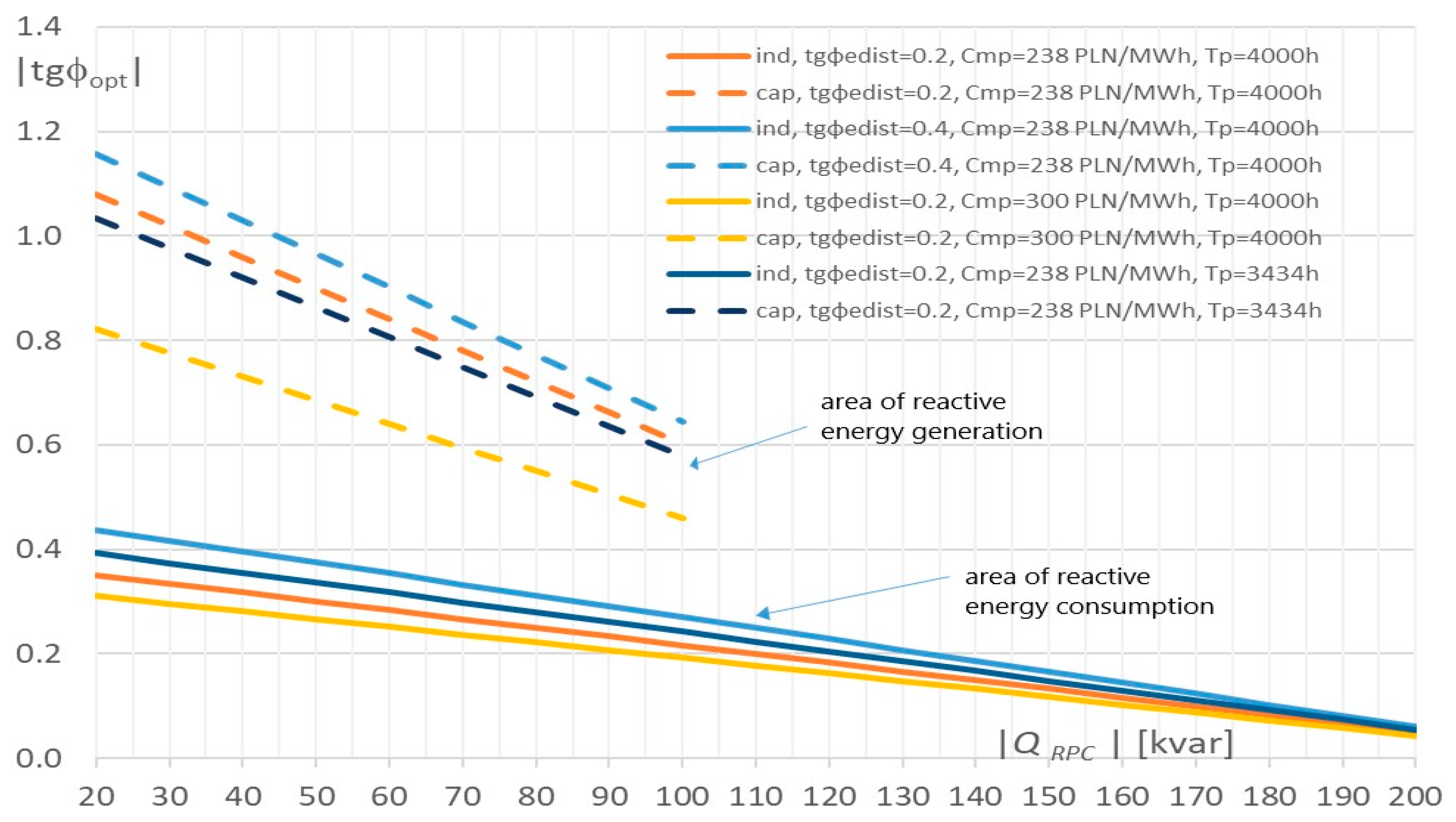
The results of the optimal tgφ_opt power factor as a function of the rated power of the reactive energy compensator are presented in Figure 1. The calculations are carried out for exclusive annual inductive or capacitive energy receivers (i.e., receivers only consume or only supply reactive energy), assuming supply from the suburban network (according to Table 3) and other selected parameters of the Formula (44) presented in Figure 1.

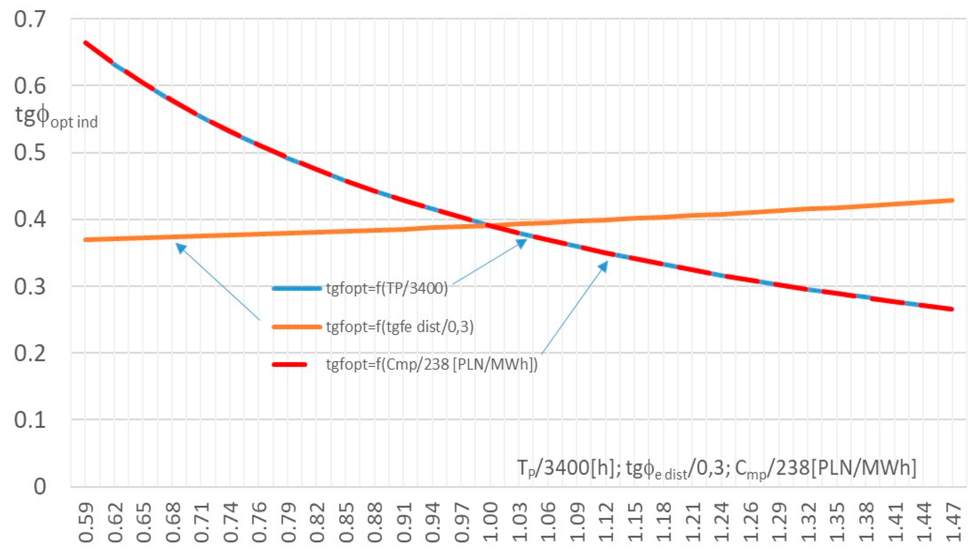
The influence of changes in individual parameters on the value of tgφ_opt is analyzed in Figure 2 in relation to the selected basic values of T_p = 3400 h, tgφ_{e dist} = 0.3 and C_mp = 238 PLN/MWh.

5. Discussion of Results

There are numerous parameters that significantly affect the optimal tgφ_opt power factor, according to Equation (44). It is proportional to the LCOE_r compensation costs and its values decrease significantly, as presented in Figure 2, with the increase in the nominal compensator power as a result of the decrease in the unit cost of reactive energy generation according to (47) and (48). The important influence on tgφ_opt value is exerted indirectly by changes in the peak load utilization time T_p, which is presented in Figure 2. Assuming there are no changes in the other parameters of Formula (45), the increase in time T_p of the supplied loads leads to the increase in reactive energy generation taking into account (49) and to the decrease in the LCOE_r value resulting in lower values of tgφ_opt values. The value of tgφ_opt is inversely proportional to the market electricity price and the low-voltage network losses expressed by ρ_LV as well as to the network losses at higher voltage levels expressed by ρ_MV and ρ_HV with a limited impact due to the application of correction factors.

Market electricity prices, which DSOs are obliged to pay to cover active energy losses in the network, influence the tgφ_opt values in an inversely proportional way. Taking into account the rapidly growing prices of CO₂ emission allowances, wholesale electricity prices in Poland are expected to increase, reducing the tgφ_opt value in the near future. The values of network losses at the low-voltage level also affect the value of tgφ_opt in an inversely proportional way, but these values are the result of the network parameters and are much more stable than the wholesale energy prices on the market in Poland. The influence of losses in medium- and high-voltage networks on the tgφ_opt value is limited due to the reduction in their impact by the parameters a and b, while a is significantly greater than b in actual distribution networks.

Changes in T_p, resulting in changes in the LCOE_r, or C_mp values between −40% and +40% cause significant changes in the tgφ_opt values within the range of +70% to −30%, but the upward trend is more acute with the relative values of the parameters analyzed below 1, while the downward trend is more moderate with their relative values above 1.

The value of tgφ_opt is also proportional to the value of the factor (1 + tg²φ_{e dist}) factor, which is related to the losses in the equivalent resistance of the power system induced by the reactive energy distribution assuming that the specific equivalent tgφ_{e dist} coefficient reflects the generation and consumption of reactive energy in the elements of the distribution network and the loads supplied taking into account their existing reactive power compensation level.

A steady increase in the optimal tgφ_opt power factor can be observed along with an increase in the characteristic of the tgφ_{e dist} value for the distribution network. As a result of tariff regulations in Poland, imposing penalty fees for customers who exceed the value of tgφ_p = 0.4, which is the permissible value within the settlement period, the value of the tgφ coefficient of the average network load will not exceed tgφ_p = 0.4 (inductive) due to the operation of compensation devices. The value of tgφ_p may only be lower due to a large group of receivers that do not require compensating devices due to their natural power factor tgφ < 0.4. The increasing level of tgφ_{e dist} value in the distribution network leads to a decrease in the equivalent resistance value of the distribution system, because the statistical losses do not change assuming stable active power consumption by loads, while the losses caused by the flow of reactive energy increase, forcing R_en to reduce the level of computational losses to their statistical values. The decreasing R_en enables a greater inflow of reactive energy through the grid and simultaneously a reduction in the needed reactive energy generation in the compensation process by customers. When tgφ_{e dist} is reduced from 0.4 to 0.2, the values of tgφ_opt decrease by approximately 10%.

Equation (44) was established with the assumption that the load parameters of the MV grid, such as the peak load utilization time T_p and the peak loss time τ_a, are the same for the MV and LV network, which is undoubtedly a simplification, but it is necessary due to the limited availability of data on T_p in MV power lines unlike the parameters of the HV/MV and MV/LV transformers. The database for the transformers may be further expanded due to the ongoing load recording at HV/MV substations as well as at MV/LV substations with the balancing meters installed at the low-voltage side of the transformers. The registration of T_p values for MV lines connected to HV/MV substations becomes possible with the ongoing installation of modern bay digital control units in the feeder bays of HV/MV substations, but at present, the data from such units are not available in Poland. In the event of availability of T_p for MV feeders, it may be used in Formula (19) for tgφ_opt calculations.

For the peak powers modeled of urban, suburban and rural networks with the assumed peak load utilization times and peak loss times presented in Table 3 and for T_p = 4000 h influencing the LCOE_r value, a slight variation of the optimal tgφ_opt values within the limits of ±2% can be observed due to the type of network. Lower values may be observed for urban networks and higher values may be observed for rural networks, which is the result of substantially higher losses in urban networks compared to losses in rural networks assuming average peak loading of these networks.

The presented method used to determine tgϕ_opt is the alternative to that used until now, involving the analysis of active energy losses in the distribution system modeled in the computational packages used to calculate power flow in power networks. Such a method of hourly power flow calculations for changing levels of reactive energy compensation of supplied loads assumes detailed knowledge of network parameters as well as the network structure throughout the year, which may change as a result of operational management of the network.

In the presented methodology, we use the annual losses in the network resulting from the balance of smart meter readings in the MV/LV station and the aggregated profiles of hourly loads of consumers as well as the network resistance equivalent determined on the basis of the balance of annual energy at individual voltage levels of the distribution network. Therefore, we rely on the real annual losses that occurred in the network as a result of the loads with different energy consumption profiles that occurred in this network without a detailed mapping of the network structure.

The results of both methods should give comparable results. The differences may result from the lack of accuracy in mapping network parameters in the power flow analysis methodology and from errors in meters recording active energy flows in various points of the network and at consumer installations being the basis of losses considered using the presented method. Attention should also be paid to the computational complexity of the load flow methodology, which requires carrying out 8760 calculations of power flows with hourly registration of losses for every level of reactive energy compensation to choose the optimal one and mapping changes in the network structure along with the exact parameters of these changes. Therefore, we rely on annual real energy loss balances and not on the calculation of power flows based on the network model.

6. Practical Application of the Results

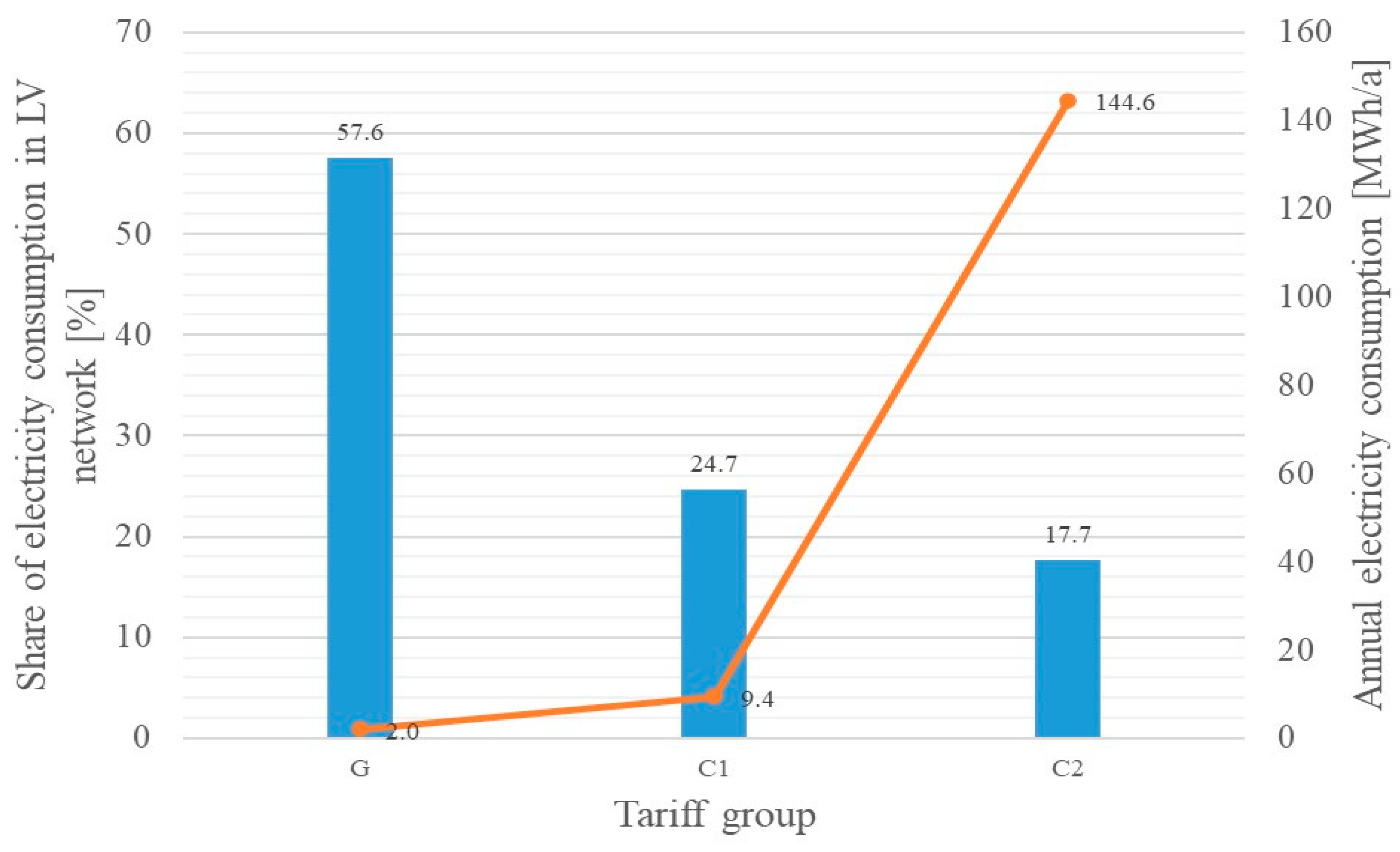
In conclusion of the results obtained, it is important to select an acceptable tgφ factor for consumers to keep, the maintenance of which would not result in penalties for excessive reactive energy consumption and which could be approved by regulatory authorities in DSO electricity tariffs. There are various groups of consumers in the low-voltage grid from small households to commercial and industrial consumers using significant amounts of energy. The percentage share of different types of consumers in total low voltage consumption in the Polish grid is presented in Figure 3 based on data for the five largest DSOs connected to the transmission network in 2019 [76]. The G tariff group is used by household consumers, the C1 tariff is used to settle small companies, while the C2 tariff is for larger commercial or industrial consumers. Figure 3 also presents the average annual electricity consumption of the consumers settled according to the considered LV tariff group. According to Figure 3, the dominant energy consumers are households exceeding 55%, while the C2 tariff group customers account for less than 20% and the C1 tariff group customers account for less than 25% of the total electricity consumption in the LV network.

To properly choose the reactive energy compensation devices, it is necessary to consider the peak load power values P_p, which are used to determine the rated powers Q_p of the compensation devices according to (34). The peak loads of consumers can be estimated as a ratio of their annual energy consumption and the maximum load utilization time. For residential consumers, according to [77], the T_p times equal a maximum of 3000 h, while for commercial and industrial customers, they may exceed 4000 h. For households, assuming annual electricity consumption according to Figure 3 and T_p = 3000 h, the average hourly peak loads do not exceed 1 kW, resulting in compensator capacities lower than 1 kvar even for large natural tgφ values. Although the natural tgφ factor of residential consumers is usually lower than 0.4, even customers with higher tgφ_p values would result in compensator devices with really small rated powers and the following high utilization costs. Therefore, it is advisable to exempt these low-voltage residential consumers from the obligation to maintain the contractual tgφ value at a permissible level.

In case of C2 group customers, for annual energy consumptions presented in Figure 3 and the peak load utilization times varying from 3000 to 4000 h, peak load values range from 35 to 50 kW. Natural tgφ_p coefficients for such loads amount to approximately 1.0, while the optimal tgφ_opt values presented in Figure 1 vary between 0.3 and 0.4. The rated capacities of reactive power compensators for such consumers, obtained as a result of the multiplication of the peak load P_p and the difference of natural and optimal tgφ values, are within the range of 20 to 40 kvar. Therefore, for this group of consumers, the obligation to maintain the tgφ_opt factor at its optimal value is justified.

In the case of commercial and industrial customers in the C1 group (P ≤ 40 kW), decisions about the obligation to compensate excessive reactive energy should be made individually, depending on the customer’s tgφ_p power factor and the required capacity of the reactive energy compensation devices to be applied, which determines the viability of the compensation.

Due to the high costs of inductive reactive energy generation, the compensation of consumers using capacitive reactive energy (introducing reactive energy into the grid) is optimal with much higher tgφ_opt coefficients exceeding 0.8 for compensators’ rated power ranging from 30 to 50 kvar. Usually, introducing the capacitive reactive energy to the grid takes place at night as a result of using receivers with power electronic control of energy consumption being at no load state or the usage of modern lighting devices using LED sources. The levels of capacitive energy consumption are rather low in such cases, so the use of capacitive reactive energy compensators, taking into account the network losses only, is not economically justified.

However, accepting the high values of the capacitive tgφ_{opt g} power for consumers can provoke them to change their consumption of reactive energy toward its generation to the grid as a result of the adequate connection of the fixed capacitor within the receiving installations. The network losses could then reach higher values than for the originally determined optimal inductive tgφ_{opt c} values, and the consumer could avoid installing a regulated inductive power compensator, as the optimal levels for reactive power generation are high. The high natural tgφ values of the loads in terms of reactive energy generation, not limited by the high optimal tgφ_opt values obtained based on the presented methods, can also jeopardize as well the DSO voltage regulation strategy, particularly for networks with a significant share of distributed renewable energy sources. In order to prevent such actions and their possible consequences, it may be necessary to apply the rule of limited or zero reactive energy feed into the grid.

$$tg{\phi }_g\approx 0$$

(50)

Currently, for many electricity consumers, variations between the consumption and generation of reactive energy may be observed even within the basic market settlement period of one hour. Such consumers should limit the excessive consumption of reactive energy, as well as its generation, to the grid at the permissible levels.

7. Conclusions

The methodology to determine the optimal levels of reactive energy flows in distribution networks presented in this article results in the optimal tgφ_opt factor of the customers as a function of the costs of DSOs to cover network losses, the costs of reactive energy compensators for consumers, the characteristics of the network load T_p, P_p, τ_P and τ_S, and the equivalent resistance originally determined of the supply network Ren. To determine this equivalent resistance, statistical data on the efficiency of distribution grid operation at individual voltage levels are used, and the average power factor level in this grid is assumed. The optimal level of reactive energy compensation for consumers connected to the low-voltage distribution network is calculated based on the costs of compensation devices, which were obtained from the study of compensation providers on the Polish market. In addition, an analysis of the change in various parameters that influence the optimal tgφ_opt value is also presented, and the rationality of applying various requirements in respect of reactive energy compensation for consumers with different contracted power levels is also discussed. The presented methodology and the obtained results allow one to formulate the following conclusions.

• The optimal compensation level of the customer load is strongly dependent on the price of electricity purchased by the DSO to cover network losses and also on the costs of using reactive energy compensation devices, which decrease with the rated power of the compensator applied; an increase in energy prices and a reduction in compensating device costs lead to a reduction in the optimal levels of the tgφ_opt factor.
• The cost of using compensating devices is inversely proportional to their power Q_RPC and to the maximum load utilization time of the compensated receivers T_p, as a consequence of higher efficiency in case of using compensation devices for heavier loads; for compensators of smaller capacities, needed for typical households, the costs of individual compensation are high, leading to optimal tgφ_opt factors higher than the natural factors for such consumers; therefore, individual compensation in the case of households is not advisable.
• For commercial customers with contracted power exceeding 40 kW, the level of inductive reactive energy compensation under the current market conditions is around tgφ = 0.3, which is lower than the permissible value of 0.4 currently applicable in the DSO tariffs in Poland.
• The equivalent resistance values of the supply system, calculated downstream of the MV busbars or downstream of the LV busbars, based on the annual losses registered by the energy-balancing meters at a voltage level of the distribution network, are the precise reflection of long-term real losses within the considered part of the distribution system.
• The values of the optimal tgφ factors obtained based on the minimization of supply cost limit the natural tgφ values of commercial and industrial loads in terms of inductive reactive energy consumption so that they limit the voltage drops; that is why they do not cause excessive voltage drops in the distribution network especially in the case of a low-voltage network taking into account its low equivalent reactance; the optimal permissible values of reactive energy injections into the grid or capacitive consumptions are much higher, but their sharp limitation is proposed by Formula (50) in case of voltage regulation problems or expected customer artificial shift to reactive power generation.
• In case of any violation of the allowed voltage limit, the DSO, based on its own load flow studies, should introduce special measures, e.g., the introduction of reactive power at certain points of the network, and this problem should be solved by the DSO operation services of the DSOs on a regular basis if the optimal reactive power compensation levels lead to voltage deviations greater than ±10% in 95% of periods of ten minutes of a week [5].
• The presented method can be considered a simple alternative to determine the optimal reactive energy compensation parameters, which can otherwise be obtained using power flow studies, and it is based on network structure, loads and local generation models simulating the analyzed periods of network operation, using the registered energy losses and load parameters in the network in the previous annual periods which can be considered as sufficiently accurate in a stable or slowly changing environment; the preparation of such a tool in the presented study was supported by the association of DSOs in Poland.

The formula determining the optimal levels of reactive energy flow to consumers allows one to use the growing amount of data from smart metering systems installed at HV/MV and MV/LV substations, which are capable of recording energy flows in the basic market settlement periods. The periodic measurements registered in the AMI systems allow the determination of network parameters such as the peak load utilization time T_p or the peak loss times τ_P replacing the integration of power values that change over time with the sum of the AMI registered values for selected network areas, and they may allow the application of the results of the presented methodology with great confidence. The results presented concern the network parameters in the analyzed past periods and constitute the basis for determining the optimal values of the tgϕ coefficient of consumers, which should be verified annually in future periods based on current loads and energy loss balances.

Additionally, the formulas presented to determine the equivalent resistance of the supply path enable the calculation of the costs of avoided losses due to the application of compensation along the network feeders and thus allow the evaluation of the value of reactive energy ancillary services provided by the distributed generation for the DSOs. The valuation of such services, as well as the monitoring and explanation of the network equivalent resistance changes due to the increasing level of distributed generation or energy storage connected to the network, may constitute an extension of the currently presented results.