Modeling and Harmonic Analysis of a Fractional-Order Zeta Converter

Abstract

The Zeta converter is an essential and widely used high-order converter. The current modeling studies on Zeta converters are based on the model that devices, such as capacitors and inductors, are of integer order. For this reason, this paper takes the Zeta converter as the research object and conducts an in-depth study on its fractional-order modeling. However, the existing modeling and analysis methods have high computational complexity, the analytical solutions of system variables are tedious, and it is difficult to describe the ripple changes of state variables. This paper combines the principle of harmonic balance with the equivalent small parameter method (ESPM); the approximate analytic steady-state solution of the state variable can be obtained in only three iterative steps in the whole solving process. The DC components and ripples of the state variables obtained by the proposed method were compared with those obtained by the Oustaloup’s filter-based approximation method; the symbolic period results obtained by ESPM had sufficient precision because they included more combinations of higher harmonics. Finally, the influence of fractional order on harmonics were analyzed. The obtained results show that the proposed method has the advantage of being less computational and easily describing changes in the ripple of the state variables. The simulation results are provided for validity of the theoretical analysis.

1. Introduction

Since the development of electronic converters of a high frequency and high integration of power, the scale and complexity of the systems continue to increase. Thus, the errors caused by modeling gradually cannot be ignored. Inductance and capacitance are essential energy storage components in DC-DC converters. Most modeling and analysis methods for DC-DC converters is based on integer order inductors and capacitors. The literature [1,2] shows that inductance and capacitance are both fractional order in nature, which means that errors may occur inevitably when using the integer-order model to analyze inductance and capacitance. Research on more accurate modeling and analysis methods for DC-DC converters have important theoretical significance and practical application value.

Low-order converters, such as buck, boost, and buck-boost converters, have the advantages of a small size, simple structure, and high conversion efficiency, which can easily achieve boost, step-down, and negative voltage output. They are widely used in inverter circuits and power factor correction circuits (PFC). References [3,4,5] use fractional-order calculus theory to model and analyze boost converters operating in continuous conduction mode (CCM), discontinuous conduction mode (DCM), and pseudo-continuous conduction mode (PCCM), respectively. In references [6,7], the fractional-order mathematical model and the state average model of CCM and DCM buck converters were established and analyzed, respectively, based on fractional calculus theory. The research results show that the fractional-order models of boost converters and buck converters based on fractional-order calculus theory differ greatly from those of integer-order models. Compared with the integer-order model, the fractional-order model is more accurate and more consistent with the actual circuit essence. At present, there are mainly four definitions of fractional calculus. The research result under different definitions of fractional order calculus is also different. References [8,9] conducted a steady-state analysis of buck converters and buck-boost converters in CCM mode based on Riemann Liouville’s (R-L) calculus definition and compared the results with the analysis results defined by Caputo. Compared with the Caputo definition, using the R-L definition to analyze the fractional buck converter and buck-boost converter is more accurate, and better in tracking dynamic response. However, different definitions of fractional-order calculus are not as unified as those of integer-order calculus, and it is difficult to give the expression of the analytical solution of the system according to these definitions [10,11]. Therefore, numerical algorithms can be used to solve and analyze fractional-order systems. The existing modeling methods of the fraction-order converter include the state space averaging method, predictive correction method (ABM), and the Oustaloup’s frequency-domain filtering method. The state-space averaging method takes the single period of the system as the research object. According to the state-space equations of the system equations in different modes, weighted average processing is performed on the linear switching function in each period, and then through the small signal disturbance processing and linearization processing, the equivalent model of the switching converter is obtained. Since the state space averaging method is “averaging” processing, and only considers the low-frequency characteristics of the system, ignoring the high-frequency dynamic characteristics of the switching converter, which will fail to correctly analyze the steady-state characteristics of the system, especially considering that the inductance and capacitance are fractional order, the inductance current ripple and capacitance voltage will be larger than the integer order. So, the error is bigger in fractional circuits. The basic idea of ABM is to establish the time model of the system, obtain the fractional differential equation of the system, then to discretize the differential of the equation, and then obtain the near value of the numerical solution through the pre-estimator, and the initial value of the next iteration can be obtained by using the corrector obtained in the calculation process. After many iterations, the numerical solution gradually converges to a stable numerical interval. The advantage of the ABM algorithm is its simple and effective nature, but due to the restriction of time complexity, the selection of initial value and the dimension of variables will affect the system’s analysis of the research. The Oustaloup frequency-domain filtering method can clearly express the relationship between system state variables and circuit element parameters when analyzing fractional order systems. However, the Oustaloup’s frequency-domain filtering method also has some problems, such as difficulty in modeling high-order converters, slow running speed and the impact of switching frequency on simulation results. The lower limit of fitting frequency, upper limit of fitting frequency and the order of filter also have great influence on the accuracy of fractional-order DC-DC converter modeling. The fractional calculus operation has long-term memory characteristics, which results in the numerical algorithm occupying a large memory space and the operational process being time-consuming in simulating computer software [12]. References [13,14] use ESPM to model and analyze the steady-state characteristics of fractional-order buck and boost converters in CCM and DCM. Using the ESPM, the approximate steady-state analytical solution of the state variables can be obtained without considering the complex definition of fractional calculus, and the amplitudes of each harmonic in the circuit can be calculated. Compared with the numerical solution, the analytical solution obtained by ESPM is more general and can reflect the relationship between the system state variables better and more intuitively. In addition, the ESPM has the advantages of fast running speed and less memory.

Now, the fractional order modeling and analysis of converters are mainly focused on low-order converters. However, high-order converters (Cuk, Sepic, Zeta) can achieve higher voltage gain, small ripple, small volume, and higher transmission efficiency, so they are widely used in wind power generation systems, fuel cells, and photovoltaic systems [15,16,17]. However, the modeling and analysis methods for high-order converters are very complicated [18]. The research and analysis on the modeling of Zeta converters has been achieved to some extent, but the research results are mainly based on the model that the capacitors and inductors in the circuit are of integer order. Therefore, in this paper, we take the Zeta converter as the research object and conduct an in-depth study on its fractional-order modeling. Based on the existing research, we consider the fractional-order characteristics of capacitors and inductors in the circuit and analyze the characteristics of fractional-order circuits, which not only can represent the real characteristics of the converter more accurately, but also can use the nature of fractional-order calculus to expand its application scope and further improve the performance of the converter. In this way, we can improve the theoretical basis of power electronic converter circuit research. For this reason, this paper aims to model and analyze the fractional order Zeta converter operating in CCM by using ESPM and proposes a method for obtaining approximate analytical solutions of the state variables of the inductor current and capacitor voltage. According to the obtained solutions, the DC quantity, ripple, and harmonics of the state variables can be analyzed intuitively, and then the relative performance of the DC chopper can be studied.

This paper is organized as follows. Section 2 deals with the modeling of the fractional-order Zeta converter in CCM. Section 3 establishes an equivalent model based on the ESPM method and the approximate solution. In Section 4, simulations are performed to verify the proposed method. The effects of fractional order on the harmonic amplitude of capacitor voltage and inductor current are discussed in Section 5. Finally, conclusions are given in Section 6.

2. Mathematical Model of the Fractional CCM Zeta Transformer

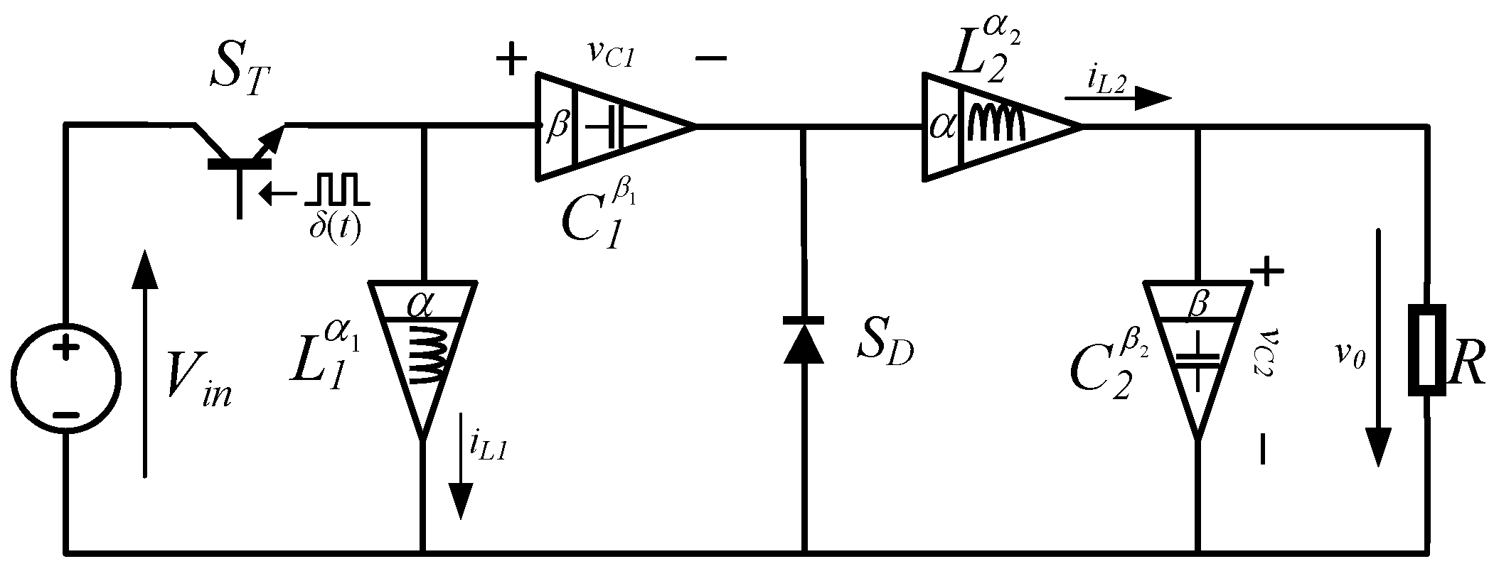
The circuit topology of the fractional Zeta converter is shown in Figure 1. In the figure, V_in is the power supply voltage, δ(t) is the switching function, S_T and S_D are the switching tubes, R is the circuit resistance, and i_L1, i_L2, v_C1 and v_C2 are the inductive current and capacitor voltages of the converter, respectively. α and β are the orders of the inductor and capacitor, respectively.

The fractional-order inductor and the voltage across the capacitor have the following relationship:

$$\left\{\begin{array}{l}{v}_L(t)=L\frac{d^{\alpha }{i}_L}{d{t}^{\alpha }}\hfill \\ i_C(t)=C\frac{d^{\beta }{v}_C}{d{t}^{\beta }}\hfill \end{array}\right.$$

(1)

When both α and β are equal to 1, the object being modeled is a traditional integer order model.

When the converter operates in the continuous current mode (CCM), the switches S_T and S_D are controlled by the switching function δ(t). The fractional-order Zeta converter has two operating modes in one switching period T_S. The inductor current and capacitor voltage are used as the state variables of the converter; fractional-order differential equations describe the state variables of the two modes of the converter:

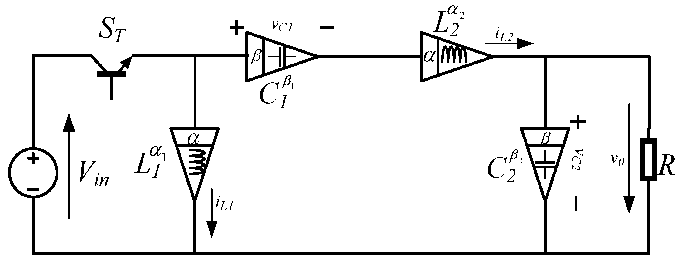
Mode 1: $n{T}_S<t\le (n+D)T_S$, where D is the on-time duty cycle and n is an integer representing a certain switching period. As shown in Figure 2, at this time δ(t) = 1, S_T is turned on and S_D is turned off, and the state equation is written:

$$\left\{\begin{array}{l}\frac{{\mathrm{d}}^{\alpha 1}{i}_{L1}}{\mathrm{d}{t}^{\alpha 1}}=\frac{v_{in}}{L_1}\\ \frac{{\mathrm{d}}^{\alpha 2}{i}_{L2}}{\mathrm{d}{t}^{\alpha 2}}=\frac{v_{in}-v_{C1}-v_{C2}}{L_2}\\ \frac{{\mathrm{d}}^{\beta 1}{v}_{C1}}{\mathrm{d}{t}^{\beta 1}}=\frac{i_{L2}}{C_1}\\ \frac{{\mathrm{d}}^{\beta 2}{v}_{c2}}{\mathrm{d}{t}^{\beta 2}}=\frac{i_{L2}}{C_2}-\frac{v_{c2}}{R{C}_2}\end{array}\right.$$

(2)

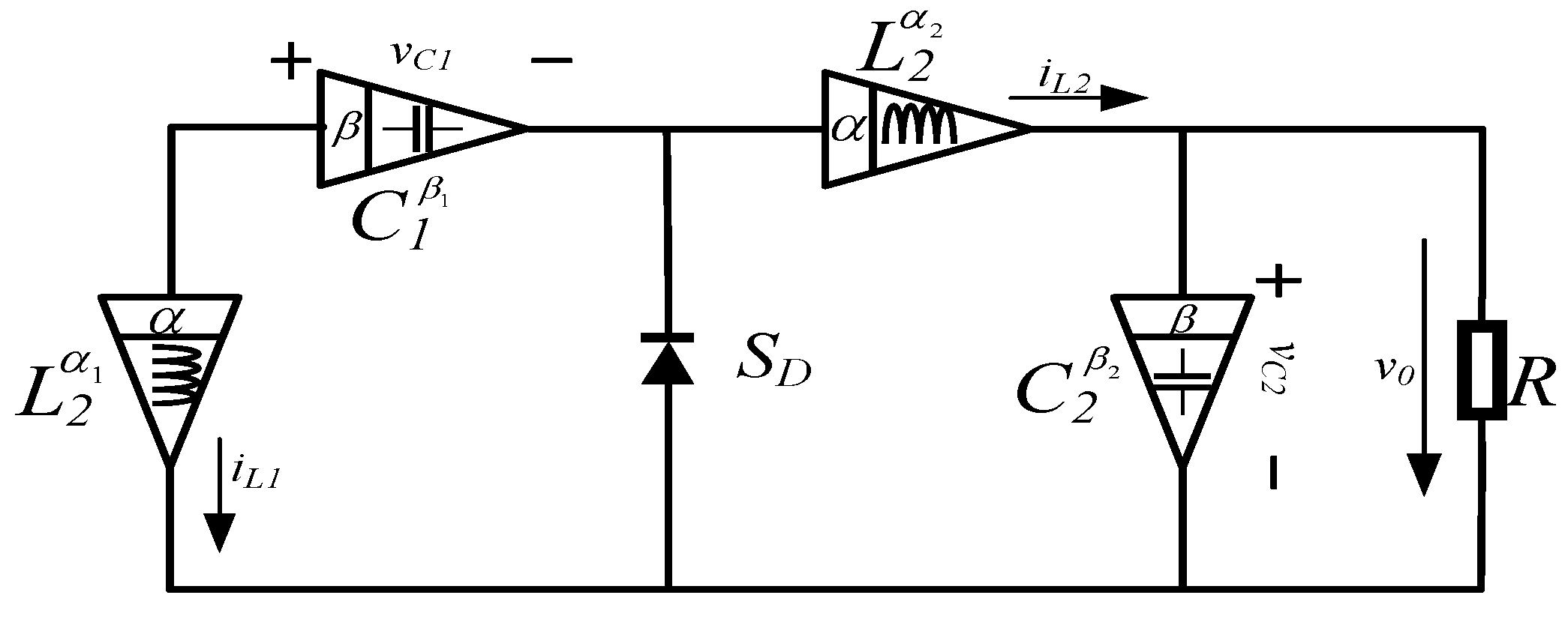
Mode 2: $(n+D)T_S<t\le (n+1)T_S$, at this time δ(t) = 0, S_T is turned off and S_D is turned on. As shown in Figure 3, the state equation is written as:

$$\left\{\begin{array}{l}\frac{{\mathrm{d}}^{\alpha 1}{i}_{L1}}{\mathrm{d}{t}^{\alpha 1}}=\frac{v_{\mathrm{C}1}}{L_1}\\ \frac{{\mathrm{d}}^{\alpha 2}{i}_{L2}}{\mathrm{d}{t}^{\alpha 2}}=-\frac{v_{c2}}{L_2}\\ \frac{{\mathrm{d}}^{\beta 1}{v}_{C1}}{\mathrm{d}{t}^{\beta 1}}=-\frac{i_{L1}}{C_1}\\ \frac{{\mathrm{d}}^{\beta 2}{v}_{C2}}{\mathrm{d}{t}^{\beta 2}}=\frac{i_{L2}}{C_2}-\frac{v_{c2}}{R{C}_2}\end{array}\right.$$

(3)

In this paper, the operator symbols p^α and p^β are used to replace d^α/dt^α and d^β/dt^β, respectively; the nonlinear switching function δ(t) is used to represent the different modes of the fractional-order CCM Zeta converter, which is defined as:

$$\delta (t)=\left\{\begin{array}{c}1,n{T}_S<t\le (n+D)T_S\\ 0,(n+D)T_S<t\le (n+1)T_S\end{array}\right.$$

(4)

According to the mathematical model of the two modes of Equations (2) and (3) and the switching function δ(t), the differential equation of the fractional CCM Zeta converter can be obtained as

$$\left\{\begin{array}{c}{p}^{{\alpha }_1}{i}_{L_1}-\frac{v_{C_1}}{L_1}(1-\delta (t))-\frac{V_{in}}{L_1}\delta (t)=0\\ \begin{array}{l}{P}^{{\alpha }_2}{i}_{L_2}+\frac{v_{C_1}}{L_2}\delta (t)+\frac{v_{C_2}}{L_2}-\frac{V_{in}}{L_2}\delta (t)=0\\ P^{{\beta }_1}{v}_{C_1}-\frac{i_{L_2}}{C_1}\delta (t)+\frac{i_{L_1}}{C_1}(1-\delta (t))=0\\ P^{{\beta }_2}{v}_{C_2}-\frac{i_{L_2}}{C_2}+\frac{v_{C_2}}{R{C}_2}=0\end{array}\end{array}\right.$$

(5)

Representing Formula (5) in the form of a matrix equation, we have:

$$G_0(p^{{\alpha }_1},p^{{\alpha }_2},p^{{\beta }_1},p^{{\beta }_2})x+G_{1}f(x)-G_{2}t(x)=0$$

(6)

There are nonlinear functions f(x) = δ(t)x, t(x) = δ(t)e, and $e={\left[\begin{array}{cccc}\frac{V_{in}}{L_1}& \frac{V_{in}}{L_2}& 0& 0\end{array}\right]}^T$ in Formula (6), and the coefficient matrix G₀(p^α1, p^α2, p^β1, p^β2), G₁, G₂ are, respectively,

$$G_0(p^{{\alpha }_1},p^{{\alpha }_2},p^{{\beta }_1},p^{{\beta }_2})=\left[\begin{array}{cccc}{p}^{{\alpha }_1}& 0& -\frac{1}{L_1}& 0\\ 0& p^{{\alpha }_2}& 0& \frac{1}{L_2}\\ \frac{1}{C_1}& 0& p^{{\beta }_1}& 0\\ 0& -\frac{1}{C_2}& 0& p^{{\beta }_2}+\frac{1}{R{C}_2}\end{array}\right]$$

(7)

$$G_1=\left[\begin{array}{cccc}0& 0& \frac{1}{L_1}& 0\\ 0& 0& \frac{1}{L_2}& 0\\ -\frac{1}{C_1}& -\frac{1}{C_1}& 0& 0\\ 0& 0& 0& 0\end{array}\right],G_2=\left[\begin{array}{cccc}1& 0& 0& 0\\ 0& 1& 0& 0\\ 0& 0& 1& 0\\ 0& 0& 0& 1\end{array}\right]$$

(8)

The above is the state vector model of the fractional-order Zeta converter working in CCM. It can be observed that the coefficient matrix G₀(p^α1, p^α2, p^β1, p^β2) in the model is closely related to the order of the energy storage element of the converter.

3. Equivalent Model of Converter Based on ESPM

3.1. Principle of the ESPM

The ESPM is mainly based on the harmonic balance principle of solving nonlinear differential equations. By expanding the state variables of the circuit system by Fourier series, when there are enough expansion terms of the series, the sum of these series can be outstanding to approximate the periodic solution of the state variable. According to the literature [19], the generalization of the harmonic balance principle is as follows:

$$\frac{d^{\mu }{e}^{\omega \tau }}{d{t}^{\mu }}={\omega }^{\mu }{e}^{\omega \tau }$$

(9)

where µ is the order of the differential operation, which can be either an integer or a non-integer; and ω is the angular frequency of the exponential function, which can be any real number. From the above formula, it can be observed that the order of the differential operation only affects the amplitude of the differentiated exponential function but has no effect on its phase. Therefore, the harmonic balance principle can be generalized to solve fractional-order nonlinear differential equations. Furthermore, the ESPM can also be improved according to this generalization.

First, the state variable x is expanded to the form of the sum of the main oscillation component x₀ and the other corrections x_i:

$$x=x_0+{\displaystyle \sum _{i=1}^n{\epsilon }^i}{x}_i$$

(10)

The switching function δ(t) is also expanded into a similar series sum form:

$$\delta (t)={\delta }_0+{\displaystyle \sum _{i=1}^n{\epsilon }^i{\delta }_i}$$

(11)

Substituting the expansions of x and δ(t) into the nonlinear functions f(x) = δ(t)x and t(x) = δ(t)e, and then combining terms with the same order εⁱ, f(x) and t(x) can be converted to:

$$\begin{array}{l}f(x)=f_0+\epsilon f_1+{\epsilon }^2{f}_2+\dots \\ t(x)=t_0+\epsilon t_1+{\epsilon }^2{t}_2+\dots \end{array}$$

(12)

where f_i is:

$$\left\{\begin{array}{l}{f}_0={\delta }_0{x}_0\hfill \\ f_1={\delta }_0{x}_1+{\delta }_1{x}_0\hfill \\ f_2={\delta }_0{x}_2+{\delta }_1{x}_2+{\delta }_2{x}_0\hfill \\ f_3={\delta }_0{x}_3+{\delta }_1{x}_2+{\delta }_2{x}_1+{\delta }_3{x}_0\hfill \end{array}\right.$$

(13)

t_i is:

$$\left\{\begin{array}{l}{t}_0={\delta }_{0}e\hfill \\ t_1={\delta }_{1}e\hfill \\ t_2={\delta }_{2}e\hfill \\ t_3={\delta }_{3}e\hfill \end{array}\right.$$

(14)

According to the principle of harmonic balance, it can be assumed that x_i can be expressed in the form of the sum of various harmonic components shown in Equation (15):

$$x_i={\displaystyle \sum _{k\in \left\{E_{ir}\right\}}{x}_{ik}=a_{i0}+{\displaystyle \sum (a_{ik}{e}^{jk\tau }+c.c)}}$$

(15)

where c.c represents the conjugate term, and k represents the order of the harmonic, in which τ = ωt is the normalized time. a_i0 and a_ik represent the DC component of x_i and the amplitude of the kth harmonic component, respectively. In addition, the formula’s harmonic components {E_ir} are determined by the actual physical properties of the modeled object. For the DC-DC converter, due to its low-pass filtering characteristics, the main component in its state variable is DC, so set the harmonic component set {E₀} = {0} of the main oscillation component x₀. The harmonic components {E_ir} of the other corrections x_i are sequentially determined by the remainder R_i generated by the previous operation.

When the converter is in a steady state, the periodic switching function δ(t) can also be expanded into a Fourier series of the form:

$$\delta (t)=b_0+{\displaystyle \sum _{k=1}^{\infty }(b_k{e}^{jk\tau }+c.c)}$$

(16)

In the formula, $b_0=\frac{1}{T_S}{\displaystyle {\int }_0^{T_S}\delta (t)dt}=D$, $b_k=\frac{1}{2}({\alpha }_k-j{\beta }_k)$, where:

$$\left\{\begin{array}{l}{\alpha }_k=\frac{2}{T_S}{\displaystyle \underset{0}{\overset{T_S}{\int }}\delta (t)\cos (k\omega t)dt}=\frac{\sin (2k\pi D)}{k\pi }\hfill \\ {\beta }_k=\frac{2}{T_S}{\displaystyle \underset{0}{\overset{T_S}{\int }}\delta (t)\sin (k\omega t)dt}=\frac{1-\cos (2k\pi D)}{k\pi }\hfill \end{array}\right.$$

(17)

Usually, δ₀ and δ_i are taken as:

$$\left\{\begin{array}{l}{\delta }_0=b_0+b_1{e}^{j\tau }+c.c\\ {\delta }_i=b_{2i}{e}^{j2i\tau }+b_{2i+1}{e}^{j(2i+1)\tau }+c.c\end{array}\right.$$

(18)

Substitute the expansions of x_i and δ_i into f_i and t_i. Due to the multiplication of x_i and δ_i, new harmonic components are generated in f_i and t_i, as follows:

$$\left\{\begin{array}{c}{f}_i=f_{im}+\phi R_{i+1}\\ t_i=t_{im}+\phi H_{i+1}\end{array}\right.$$

(19)

Among them, f_im represents the part of f_i that is the same as the harmonic component of x_i, the remainder R_i+1 represents other components in f_i, t_im represents the part of t_i that is the same as the harmonic component of x_i, and the remainder H_i+1 represents other components in t_i components, the spectrum of x_i and R_i are the same as H_i. Therefore, the value of the x_i spectrum can be determined by R_i and H_i in the operation.

Substituting Equations (15) and (19) into Equation (6), Equation (20) can be deduced as:

$$\left\{\begin{array}{c}{G}_0{(p}^{{\alpha }_1}{,p}^{{\alpha }_2}{,p}^{{\beta }_1}{,p}^{{\beta }_2}{)x}_0{+G}_1{f}_{0m}{-G}_2{t}_{0m}=0\hfill \\ G_0{(p}^{{\alpha }_1}{,p}^{{\alpha }_2}{,p}^{{\beta }_1}{,p}^{{\beta }_2}{)x}_1{+G}_1{(f}_{1m}{+R}_1{)-G}_2{(t}_{1m}{+H}_1)=0\hfill \\ G_0{(p}^{{\alpha }_1}{,p}^{{\alpha }_2}{,p}^{{\beta }_1}{,p}^{{\beta }_2}{)x}_2{+G}_1{(f}_{2m}{+R}_2{)-G}_2{(t}_{2m}{+H}_2)=0\hfill \\ G_0{(p}^{{\alpha }_1}{,p}^{{\alpha }_2}{,p}^{{\beta }_1}{,p}^{{\beta }_2}{)x}_3{+G}_1{(f}_{3m}{+R}_3{)-G}_2{(t}_{3m}{+H}_3)=0\hfill \end{array}\right.$$

(20)

From Equation (21), the main oscillation component and each order correction can be obtained step by step. If the following conditions are met, the iteration will be stopped.

$$Tolerance=\frac{\parallel a_{ik}{\parallel }_2}{\parallel a_{00}{\parallel }_2}\le 1\%$$

(21)

By solving the equation in Equation (20), the main oscillation component and each order correction can be obtained step by step, and finally the periodic solution of the system state variable can be expressed as:

$$x=x_0+x_1+x_2+x_3\dots$$

(22)

3.2. Steady-State Analytical Solution of Fractional-Order CCM Zeta Converter

3.2.1. Solving the Main Oscillation Component x₀

Due to the low-pass performance of the DC-DC converter, it can be concluded that the main oscillation component of the state variable is:

$$x_0=a_{00}={\left[I_{00},I_{00}^{\prime },V_{00},V_{00}^{\prime }\right]}^T$$

(23)

where I₀₀, I′₀₀, V₀₀, and V′₀₀ represent the DC components of the inductor current and capacitor voltage, respectively. From Equation (19) f_i and t_i expressions, it can be expressed as:

$$\left\{\begin{array}{l}{f}_{0m}=a_{00}{b}_0\hfill \\ t_{0m}=a_{00}e\hfill \end{array}\right.$$

(24)

$$\left\{\begin{array}{l}{R}_1=a_{00}(b_1{e}^{j\tau }+c.c)\hfill \\ H_1=b_{1}e\cdot e^{j\tau }+c.c\hfill \end{array}\right.$$

(25)

Substituting Equations (24) and (25) into the first term of Equation (20), it can be expressed as:

$$G_{00}{a}_{00}+G_{1}D{a}_{00}-G_{2}De=0$$

(26)

At this time, the coefficient matrix is G₀₀ = G₀(0,0,0,0). According to the principle of harmonic balance, the above formula can be transformed into

$$\left(\left[\begin{array}{cccc}0& 0& -\frac{1}{L_1}& 0\\ 0& 0& 0& \frac{1}{L_2}\\ \frac{1}{C_1}& 0& 0& 0\\ 0& -\frac{1}{C_2}& 0& \frac{1}{R{C}_2}\end{array}\right]+D\left[\begin{array}{cccc}0& 0& \frac{1}{L_1}& 0\\ 0& 0& \frac{1}{L_2}& 0\\ -\frac{1}{C_1}& -\frac{1}{C_1}& 0& 0\\ 0& 0& 0& 0\end{array}\right]\right)\left[\begin{array}{c}{I}_{00}\\ I_{00}^{\prime }\\ V_{00}\\ V_{00}^{\prime }\end{array}\right]=D\left[\begin{array}{cccc}1& 0& 0& 0\\ 0& 1& 0& 0\\ 0& 0& 1& 0\\ 0& 0& 0& 1\end{array}\right]\left[\begin{array}{c}\frac{V_{in}}{L_1}\\ \frac{V_{in}}{L_2}\\ 0\\ 0\end{array}\right]$$

(27)

The analytical formula of a₀₀ can be obtained from Formula (27).

3.2.2. Solving the First-Order Correction Amount x₁

The components of x₁ depend on R₁ and H₁, so the set of harmonic components of the first-order correction amount x₁ is {E_1r} = {1}, and x₁ can be expressed as

$$x_1=a_{11}{e}^{j\tau }+c.c$$

(28)

Where a₁₁ = [I₁₁, I’₁₁, V₁₁, V’₁₁]^T, bring x₀, x₁, δ₀, δ₁ into f₁ and t₁, and the remainder R₂ of f_1m and f₁ can be obtained:

$$\left\{\begin{array}{l}{f}_{1m}=b_0{a}_{11}{e}^{j\tau }+c.c\hfill \\ R_2=b_1{\overline{a}}_{11}+{\overline{b}}_1{a}_{11}+(b_1{a}_{11}+b_2{a}_{00})e^{j2\tau }+b_3{a}_{00}{e}^{j3\tau }+c.c\hfill \end{array}\right.$$

(29)

Since the spectrum of H₁ is {K_1r} = {1}, the spectrum of x₁ is also {1}. In the same way, selecting the same amount as the spectrum of x₁ in t₁ as t_1m, and the other components as H₂, it can be expressed as:

$$\left\{\begin{array}{l}{t}_{1m}=0\hfill \\ H_2=b_{2}e\cdot e^{j\tau }+b_{3}e\cdot e^{j\tau }+c.c\hfill \end{array}\right.$$

(30)

Substituting f_1m, t_1m, H₁, and R₁ into the second equation of Equation (20), it can be reverted to:

$$(G_{01}+G_1{b}_0)a_{11}=(-G_1{b}_1{a}_{00}+G_2{b}_{1}e)$$

(31)

where G₀₁ = G₀[(jω)^α1, (jω)^α2, (jω)^β1, (jω)^β2], a₁₁ can be obtained by the matrix transformation of Formula (31).

3.2.3. Solve the Second-Order Correction Amount x₂

According to R₂ and H₂, it is known that the set of harmonic components of the second-order correction amount x₂ is {E_2r} = {0, 2, 3}; then, the expression of the second-order correction amount is:

$$x_2=a_{20}+a_{22}{e}^{j2\tau }+a_{23}{e}^{j3\tau }+c.c$$

(32)

The DC component in the second-order correction is a₂₀ = [I₂₀, I’₂₀, V₂₀, V’₂₀]^T, the second harmonic is a₂₂ = [I₂₂, I’₂₂, V₂₂, V’₂₂]^T, and the third harmonic is a₂₃ = [I₂₃, I’₂₃, V₂₃, V’₂₃]^T. Substituting x₀, x₁, x₂, δ₀, δ₁, and δ₂ into f₂ and t₂, it can be expressed as:

$$\left\{\begin{array}{l}{f}_{2m}=b_0{a}_{20}+(b_0{a}_{22}+{\overline{b}}_1{a}_{23}+b_3{\overline{a}}_{11})e^{j2\tau }+(b_0{a}_{23}+b_1{a}_{22}+b_2{a}_{11})e^{j3\tau }+c.c\hfill \\ R_3=(b_1{a}_{20}+{\overline{b}}_1{a}_{22}+b_2{\overline{a}}_{11})e^{j\tau }+(b_1{a}_{23}+b_3{a}_{11}+b_4{a}_{00})e^{j4\tau }+b_5{a}_{00}{e}^{j5\tau }+c.c\hfill \end{array}\right.$$

(33)

$$\left\{\begin{array}{l}{t}_{2m}=0\hfill \\ H_3=b_{4}e\cdot e^{j4\tau }+b_{5}e\cdot e^{j5\tau }+c.c\hfill \end{array}\right.$$

(34)

Bringing x₂, R₂, f_2m, H₂, and t_2m into the third formula of Formula (20), it can be expressed as:

$$\left\{\begin{array}{l}(G_{00}+G_1{b}_0)a_{20}=-G_1(b_1{\overline{a}}_{11}+{\overline{b}}_1{a}_{11})\\ (G_{02}+G_1{b}_0)a_{22}=-G_1(b_1{a}_{11}+b_2{a}_{00}+b_3{\overline{a}}_{11})+G_2{b}_{2}e\\ (G_{03}+G_1{b}_0)a_{23}=-G_1(b_1{a}_{22}+b_2{a}_{11}+b_3{a}_{00})+G_2{b}_{3}e\end{array}\right.$$

(35)

The matrix G_0k = [(jkω)^α1, (jkω)^α2, (jkω)^β1, (jkω)^β2] (k = 0, 2, 3) in Equation (35), a₂₀, a₂₂ and a₂₃ can be obtained by matrix transformation.

3.2.4. Solving the Third-Order Correction Amount x₃

According to R₃ and H₃, it can be seen that the set of harmonic components of the third-order correction amount x₃ is {E_3r} = {1, 4, 5}; then, the expression of the third-order correction amount is:

$$x_3=a_{31}{e}^{j\tau }+a_{34}{e}^{j4\tau }+a_{35}{e}^{j5\tau }+c.c$$

(36)

The fundamental harmonic, fourth harmonic, and fifth harmonic in the third-order correction amount are, respectively, a₃₁ = [I₃₁, I’₃₁, V₃₁, V’₃₁]^T, a₃₄ = [I₃₄, I’₃₄, V₃₄, V’₃₄]^T, and a₃₅ = [I₃₅, I’₃₅, V₃₅, V’₃₅]^T. Substituting x₀, x₁, x₂, x₃, δ₀, δ₁, δ₂, and δ₃ into f₃ and t₃, it can be reverted to:

$$\left\{\begin{array}{l}\begin{array}{l}{f}_{3m}=(b_0{a}_{31}+b_3{\overline{a}}_{22})e^{j\tau }+(b_0{a}_{34}+{\overline{b}}_1{a}_{35}+b_2{a}_{22}+b_5{\overline{a}}_{11})e^{j4\tau }\\ +(b_0{a}_{35}+b_1{a}_{34}+b_2{a}_{23}+b_3{a}_{22}+b_4{a}_{11})e^{j5\tau }+c.c\end{array}\hfill \\ R_4={\overline{b}}_1{a}_{31}+b_2{\overline{a}}_{22}+b_3{\overline{a}}_{23}+(b_1{a}_{31}+b_2{a}_{20})e^{j2\tau }+({\overline{b}}_1{a}_{34}+b_3{a}_{20}+b_4{\overline{a}}_{11})e^{j3\tau }+c.c\hfill \end{array}\right.$$

(37)

$$t_{3m}=0$$

(38)

Bringing x₃, R₃, f_3m, H₃, and t_3m into the fourth formula of Formula (20), it can be expressed as:

$$\left\{\begin{array}{l}(G_{01}+G_1{b}_0)a_{31}=-G_1(b_1{a}_{20}+b_3{\overline{a}}_{22}+{\overline{b}}_1{a}_{22}+b_2{\overline{a}}_{11})\\ (G_{04}+G_1{b}_0)a_{34}=-G_1(b_1{a}_{23}+b_2{a}_{22}+b_3{a}_{11}+b_4{a}_{00}+b_5{\overline{a}}_{11})+G_2{b}_{4}e\\ (G_{05}+G_1{b}_0)a_{35}=-G_1(b_0{a}_{35}+b_1{a}_{34}+b_2{a}_{23}+b_3{a}_{22}+b_4{a}_{11}+b_5{a}_{00})+G_2{b}_{5}e\end{array}\right.$$

(39)

In the coefficient matrix G_0k = G₁[(jkω)^α1, (jkω)^α2, (jkω)^β1, (jkω)^β2] (k = 1, 4, 5) in Formula (39), a₃₁, a₃₄, and a₃₅ can all be passed through matrix transformation.

According to the above process, a_ik = [I_ik, I’_ik, V_ik, V’_ik] can be obtained. According to the obtained main oscillation component x₀, first-order correction amount x₁, second-order correction amount x₂ and third-order correction amount x₃, then the analytical expression of the state vector x can be obtained as:

$$x=a_{00}+a_{20}+(a_{11}+a_{31})e^{j\tau }+a_{22}{e}^{j2\tau }+a_{23}{e}^{j3\tau }+a_{34}{e}^{j4\tau }+a_{35}{e}^{j5\tau }+c.c$$

(40)

The expressions of state variables i_L1, i_L2, v_C1, and v_C2 are:

$$\left\{\begin{array}{c}{i}_{L1}\approx (I_{00}+I_{20})+2(\mathrm{Re}{I}_{11}\cos \omega t-\mathrm{Im}{I}_{11}\sin \omega t+\mathrm{Re}{I}_{22}\cos 2\omega t\hfill \\ -\mathrm{Im}{I}_{22}\sin 2\omega t+\mathrm{Re}{I}_{23}\cos 3\omega t-\mathrm{Im}{I}_{23}\sin 3\omega t+\mathrm{Re}{I}_{31}\cos \omega t\hfill \\ -\mathrm{Im}{I}_{31}\sin \omega t+\mathrm{Re}{I}_{34}\cos 4\omega t-\mathrm{Im}{I}_{34}\sin 4\omega t+\mathrm{Re}{I}_{35}\cos 5\omega t-\mathrm{Im}{I}_{35}\sin 5\omega t)\hfill \\ i_{L2}\approx (I_{00}^{\prime }+I_{20}^{\prime })+2(\mathrm{Re}{I}_{11}^{\prime }\cos \omega t-\mathrm{Im}{I}_{11}^{\prime }\sin \omega t+\mathrm{Re}{I}_{22}^{\prime }\cos 2\omega t\hfill \\ -\mathrm{Im}{I}_{22}^{\prime }\sin 2\omega t+\mathrm{Re}{I}_{23}^{\prime }\cos 3\omega t-\mathrm{Im}{I}_{23}^{\prime }\sin 3\omega t+\mathrm{Re}{I}_{31}^{\prime }\cos \omega t\hfill \\ -\mathrm{Im}{I}_{31}^{\prime }\sin \omega t+\mathrm{Re}{I}_{34}^{\prime }\cos 4\omega t-\mathrm{Im}{I}_{34}^{\prime }\sin 4\omega t+\mathrm{Re}{I}_{35}^{\prime }\cos 5\omega t-\mathrm{Im}{I}_{35}^{\prime }\sin 5\omega t)\hfill \\ v_{C1}\approx (V_{00}+V_{20})+2(\mathrm{Re}{V}_{11}\cos \omega t-\mathrm{Im}{V}_{11}\sin \omega t+\mathrm{Re}{V}_{22}\cos 2\omega t\hfill \\ -\mathrm{Im}{V}_{22}\sin 2\omega t+\mathrm{Re}{V}_{23}\cos 3\omega t-\mathrm{Im}{V}_{23}\sin 3\omega t+\mathrm{Re}{V}_{31}\cos \omega t\hfill \\ -\mathrm{Im}{V}_{31}\sin \omega t+\mathrm{Re}{V}_{34}\cos 4\omega t-\mathrm{Im}{V}_{34}\sin 4\omega t+\mathrm{Re}{V}_{35}\cos 5\omega t-\mathrm{Im}{V}_{35}\sin 5\omega t)\hfill \\ v_{C2}\approx (V_{00}^{\prime }+V_{20}^{\prime })+2(\mathrm{Re}{V}_{11}^{\prime }\cos \omega t-\mathrm{Im}{V}_{11}^{\prime }\sin \omega t+\mathrm{Re}{V}_{22}^{\prime }\cos 2\omega t\hfill \\ -\mathrm{Im}{V}_{22}^{\prime }\sin 2\omega t+\mathrm{Re}{V}_{23}^{\prime }\cos 3\omega t-\mathrm{Im}{V}_{23}^{\prime }\sin 3\omega t+\mathrm{Re}{V}_{31}^{\prime }\cos \omega t\hfill \\ -\mathrm{Im}{V}_{31}^{\prime }\sin \omega t+\mathrm{Re}{V}_{34}^{\prime }\cos 4\omega t-\mathrm{Im}{V}_{34}^{\prime }\sin 4\omega t+\mathrm{Re}{V}_{35}^{\prime }\cos 5\omega t-\mathrm{Im}{V}_{35}^{\prime }\sin 5\omega t)\hfill \end{array}\right.$$

(41)

where Re and Im represent the real and imaginary parts, respectively.

4. Simulation Comparison and Validation of Different Methods

4.1. Design Equation of Zeta Converter

Applying Kirchhoff’s voltage law on the Zeta converter circuit for the first and second mode, the equations are derived below. The ripple of the current through the energy transferring (input) inductor can be expressed as,

$$\Delta {\mathrm{I}}_{L1}=\frac{D{\mathrm{V}}_{in}}{f_s{L}_1},L_1=\frac{D{V}_{in}}{f_s\Delta {\mathrm{I}}_{L1}}$$

(42)

The output inductor current ripple can be expressed as,

$$\Delta {\mathrm{I}}_{L2}=\frac{D{\mathrm{V}}_{in}}{f_s{L}_1},L_2=\frac{D{V}_{in}}{f_s\Delta {\mathrm{I}}_{L2}}$$

(43)

The capacitor ripple voltages ΔV_C1 & ΔV_C2 can be derived from the Kirchhoff’s current law for first and second mode as

$$\Delta V_{C1}=\frac{1}{C_1}{\displaystyle \underset{0}{\overset{T_{on}}{\int }}{i}_{C1}}dt,C_1=\frac{\mathrm{D}{V}_0}{f_s{R}_L\Delta V_{C1}}$$

(44)

$$\Delta V_{C2}=\frac{1}{C_2}{\displaystyle \underset{0}{\overset{T/2}{\int }}\frac{\Delta I_{L2}}{4}}dt,C_2=\frac{\mathrm{D}{V}_{in}}{8f_s^2{L}_2\Delta V_{C2}}$$

(45)

where V₀ = V_C2.

The simulation parameters of Figure 1 are shown in

Table 1. Simulation parameters.

Parameters	Values
Vin	12 V
R	10 Ω
D	0.4
fs	25,000 Hz
L1	2 mH
L2	2 mH
C1	10−5 F
C2	10−5 F

.

4.2. DC Components and Ripple Analysis

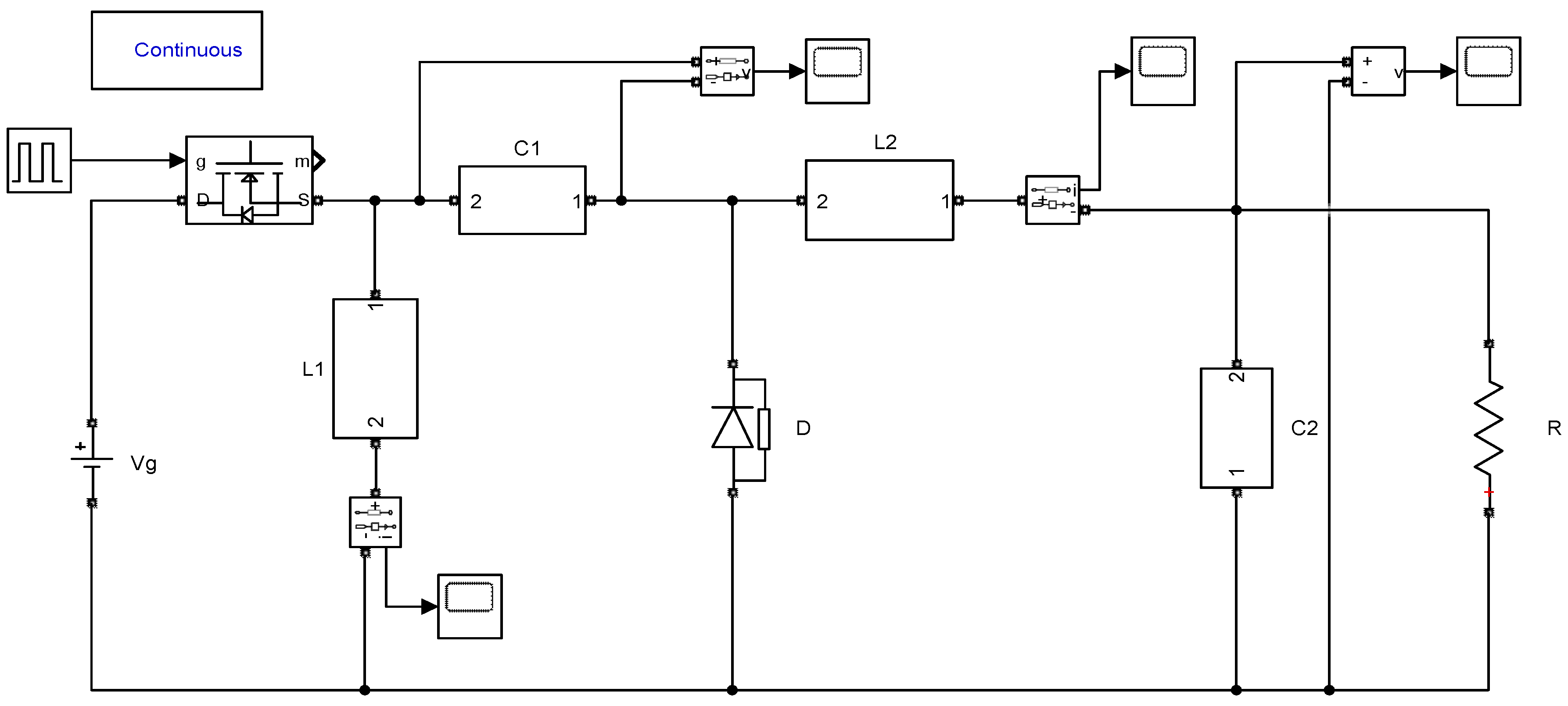
The fractional-order CCM Zeta converter is modeled on the Oustaloup’s filter-based approximation method [20], and the simulation model is shown in Figure 4.

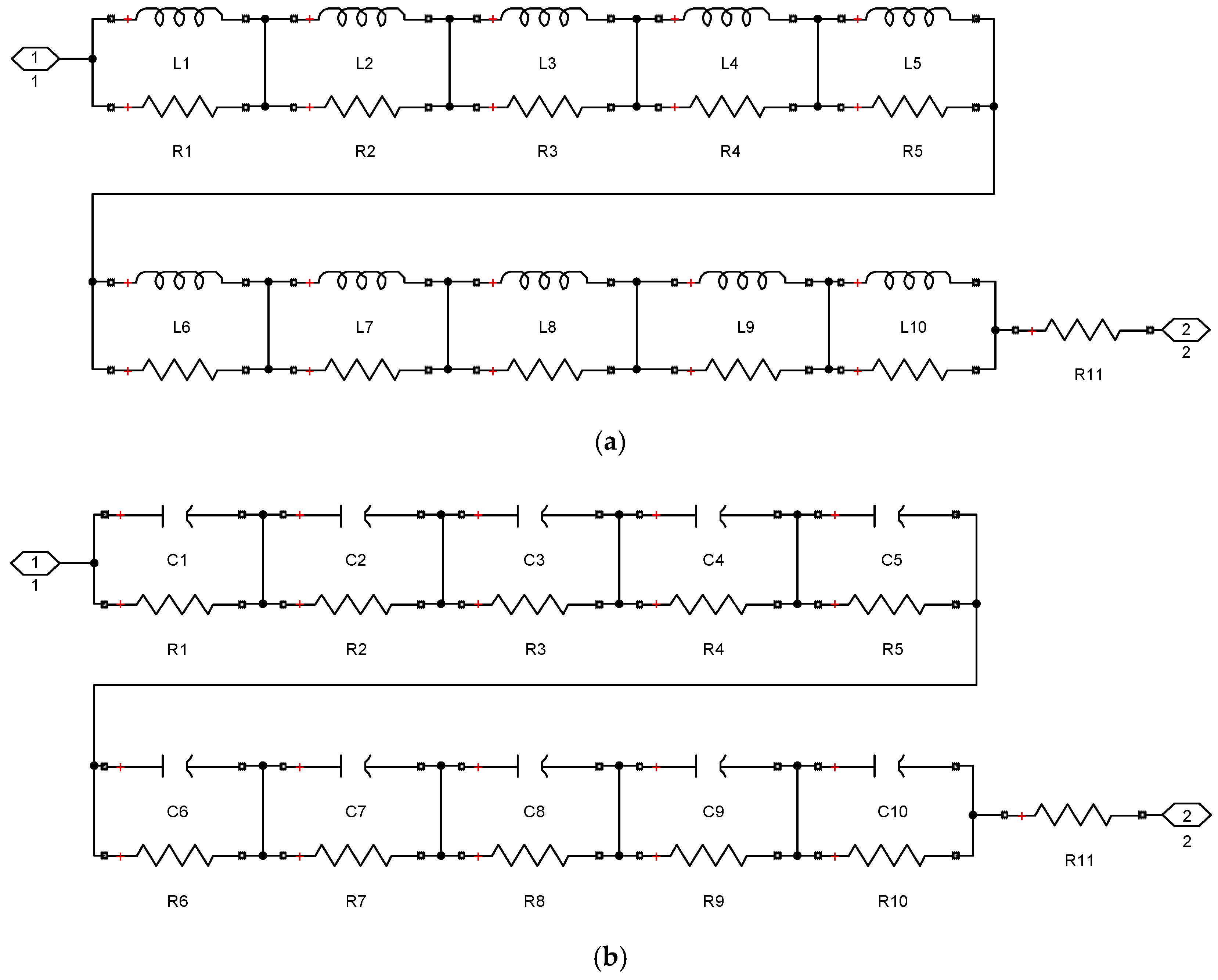
Using the Oustaloup’s filter-based approximation method, the fractional-order inductor and capacitor in Figure 4 are replaced by the equivalent circuit of the fractional-resistance chain. The fractional-resistance chain of fractional-order inductor is constructed, as shown in Figure 5a. The fractional-resistance chain of fractional-order capacitor is shown in Figure 5b.

The DC components of the state variables obtained by the Oustaloup’s filter-based approximation method and ESPM are shown in

Table 2. Comparison of DC components of state variables.

Order (α1, α2, β1, β2)	ESPM (a00 + a20)	Oustaloup’s Method
(0.85, 0.85, 0.85, 0.85)	(0.5574, 0.7515, −7.5145, 7.5145)	(0.6040, 0.7536, −7.5270, 7.530)
(0.9, 0.9, 0.9, 0.9)	(0.5417, 0.7836, −7.8359, 7.8359)	(0.5676, 0.7826, −7.8250, 7.8230)
(0.9, 0.9, 0.95, 0.95)	(0.5494, 0.7948, −7.9478, 7.9478)	(0.5813, 0.7954, −7.950, 7.950)
(0.95, 0.95, 0.95, 0.95)	(0.5354, 0.7955, −7.9546, 7.9546)	(0.5596, 0.7956, −7.9530, 7.9530)
(0.95, 0.95, 1, 1)	(0.5383, 0.7995, −7.9955, 7.9955)	(0.5625, 0.7998, −7.9940, 7.9950)
(1, 1, 1, 1)	(0.5330, 0.7998, −7.9975, 7.9975)	(0.5497, 0.8009, −7.990, 7.9970)

.

It can be seen from Table 2 that the difference between the results of the inductor current and capacitor voltage DC components obtained by ESPM and the Oustaloup’s filter-based approximation method is relatively small, and the changing trends are the same.

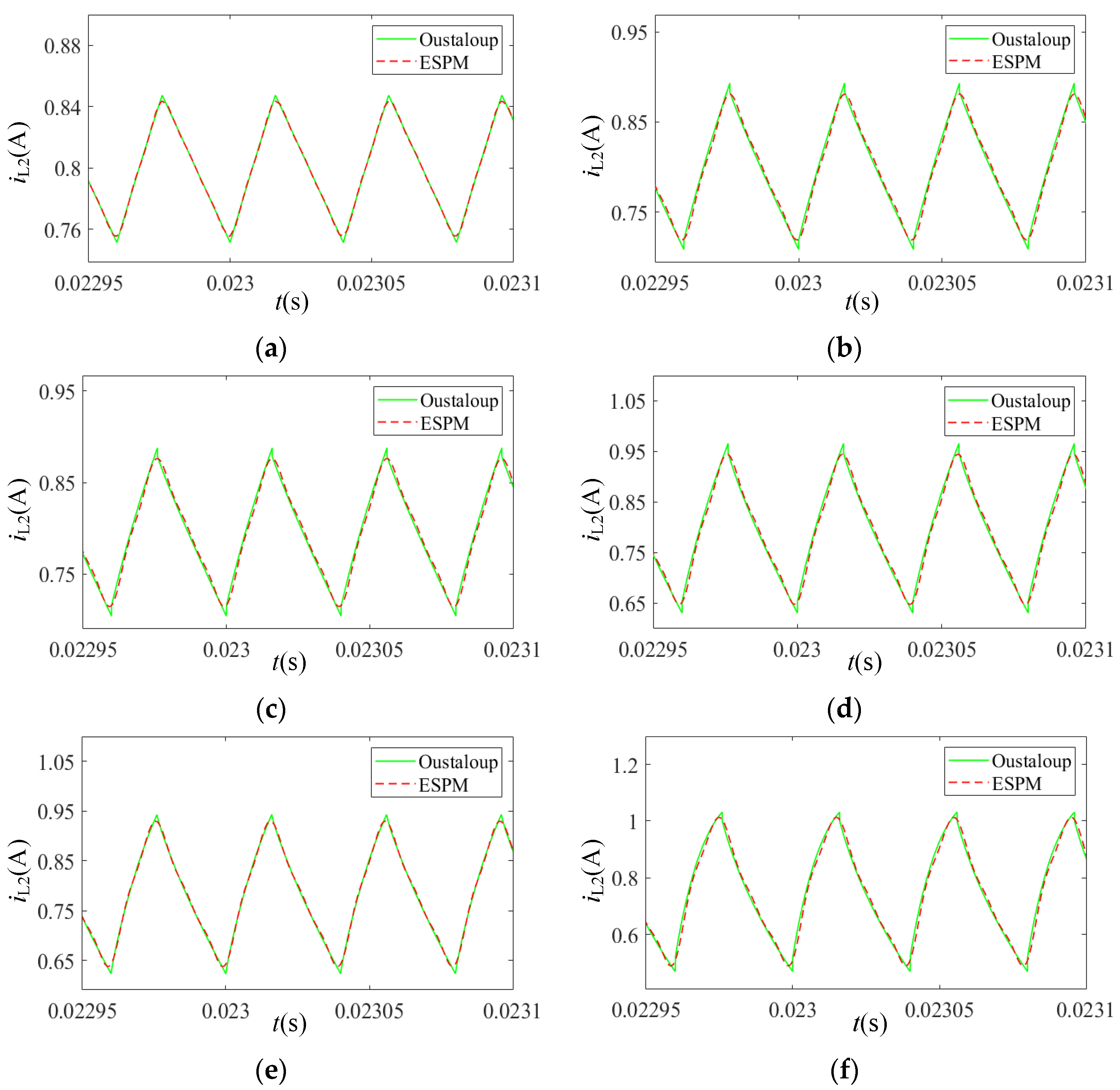
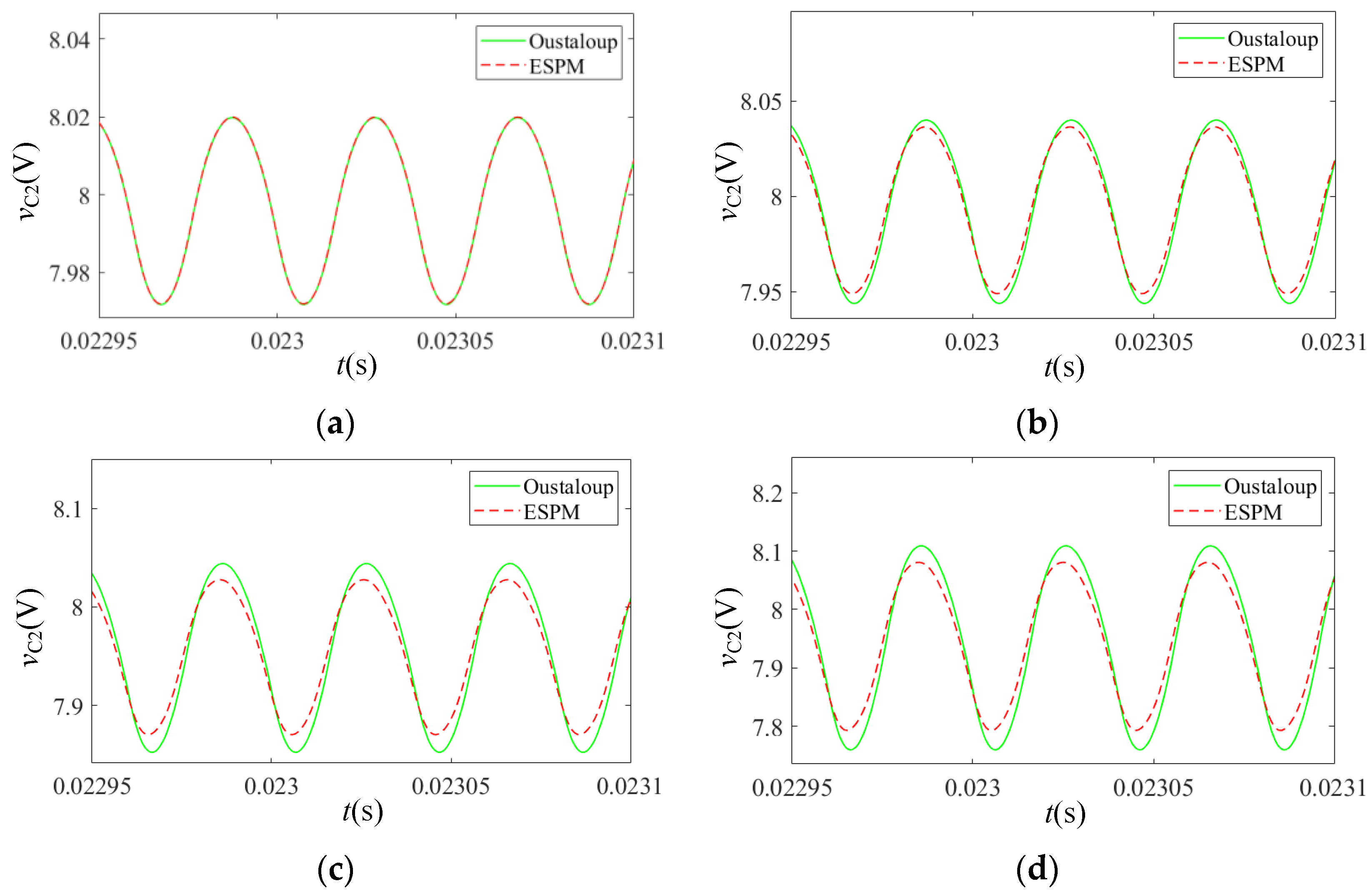
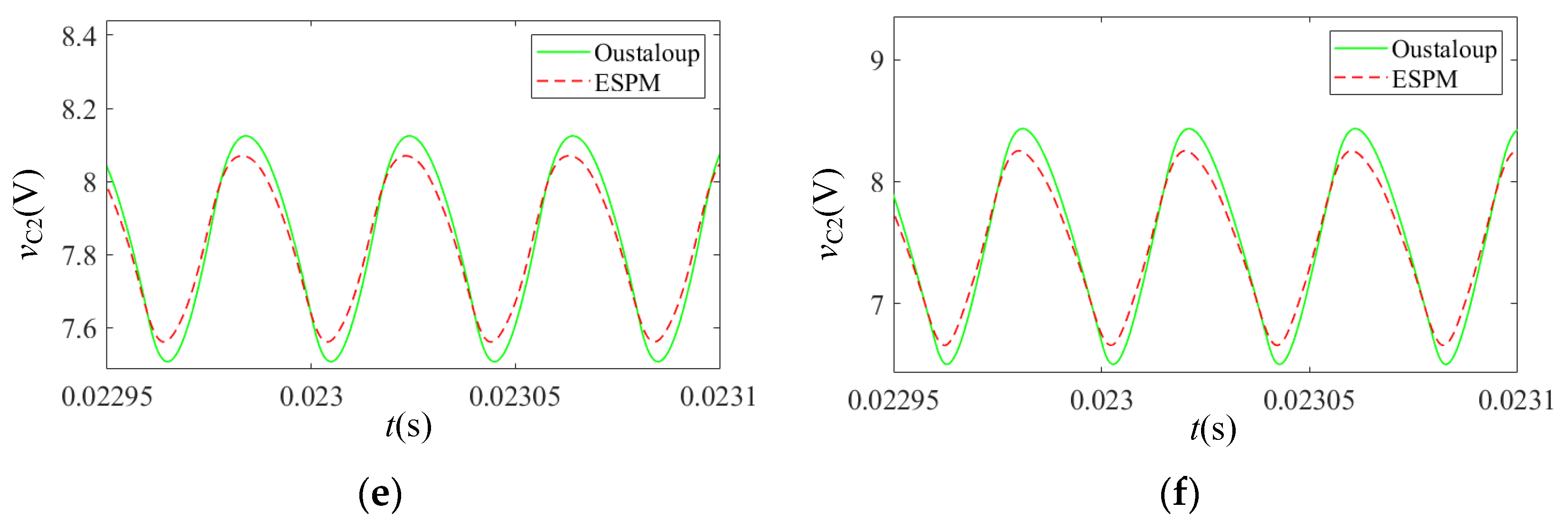
The waveform of inductor current and capacitor voltage of different orders obtained by the Oustaloup’s filter-based approximation method and ESPM are shown in Figure 6 and Figure 7, respectively. The figure’s green solid line and the red dotted line in the figure are the curves obtained by the Oustaloup’s filter-based approximation method and ESPM, respectively.

It can be seen from Figure 6 and Figure 7 that the values of the inductor current and capacitor voltage are consistent with the trends shown in Table 2. Furthermore, the steady-state ripples from the Oustaloup’s approximation method and the ESPM are compared, where the green solid lines represent the results from the Oustaloup’s approximation method, and the red dotted lines represent the results from the ESPM. The harmonic magnitudes are also order dependent. Specifically, the harmonic magnitudes of i_L and v_C increase with the decreases of α and β, respectively. Waveforms coming from these two methods show good agreement with each other, which proves the accuracy and feasibility of ESPM modeling of the fractional CCM Zeta converter.

The inductance current increment of the circuit model can be measured from Figure 6 and Figure 7, and the corresponding theoretical values can be obtained according to the formula for ripple given in Equation (46), and the comparison between the theoretical and simulated values is shown in

Table 3. Comparison of the theoretical value and the simulation value.

Order (α1, α2, β1, β2)	ΔiL	Theoretical Value	ESPM	Oustaloup
(1, 1, 1, 1)	ΔiL1/A	0.096	0.087	0.09501
	ΔiL2/A	0.096	0.0883	0.0949
(0.95, 0.95, 1, 1)	ΔiL1/A	0.1702	0.1812	0.1858
	ΔiL2/A	0.1702	0.1723	0.1851
(0.95, 0.95, 0.95, 0.95)	ΔiL1/A	0.1702	0.1853	0.1874
	ΔiL2/A	0.1702	0.1678	0.1839
(0.9, 0.9, 0.95, 0.95)	ΔiL1/A	0.3012	0.313	0.3435
	ΔiL2/A	0.3012	0.2968	0.3358
(0.9, 0.9, 0.9, 0.9)	ΔiL1/A	0.3012	0.3132	0.3435
	ΔiL2/A	0.3012	0.2918	0.3201
(0.85, 0.85, 0.85, 0.85)	ΔiL1/A	0.532	0.5716	0.5825
	ΔiL2/A	0.532	0.5246	0.5637

. The ripple error percentage is shown in

Table 4. Ripple error percentage.

Order (α1, α2, β1, β2)	ΔiL	ESPM	Oustaloup
(1, 1, 1, 1)	ΔiL1/A	9.37%	1.03%
	ΔiL2/A	8.02%	1.14%
(0.95, 0.95, 1, 1)	ΔiL1/A	6.46%	9.16%
	ΔiL2/A	1.23%	8.75%
(0.95, 0.95, 0.95, 0.95)	ΔiL1/A	8.87%	10.1%
	ΔiL2/A	1.41%	8.05%
(0.9, 0.9, 0.95, 0.95)	ΔiL1/A	3.91%	14.04%
	ΔiL2/A	1.46%	11.48%
(0.9, 0.9, 0.9, 0.9)	ΔiL1/A	3.98%	14.04%
	ΔiL2/A	3.12%	6.27%
(0.85, 0.85, 0.85, 0.85)	ΔiL1/A	7.44%	9.49%
	ΔiL2/A	1.39%	5.95%

.

Combining Table 2, Table 3 and Table 4 it can be seen that the DC components of the inductor current and capacitor voltage are basically not affected by the fractional order in a steady state. The fractional order mainly affects the ripple of the inductor current and capacitor voltage, and the ripple amplitude increases sharply as the order decreases. Analysis of the data in Table 3 shows that there is a certain error between the simulated and theoretical values, but the error is small and stays in a reasonable range. The comparison between the theoretical and simulated values fully verifies the correctness of the fractional order model and the theoretical derivation.

4.3. Fractional-Order Zeta Converter CCM Discriminant

From the method of reference [21], the expressions for the fractional order inductance currents Δi_L1 and Δi_L2 can be obtained as:

$$\left\{\begin{array}{l}\Delta i_{L1}=\frac{V_{in}{(DT)}^{{\alpha }_1}}{L_1{\alpha }_1\Gamma ({\alpha }_1)}\hfill \\ \Delta i_{L2}=\frac{(V_{in}-V_{C1}-V_{C2}){(DT)}^{{\alpha }_2}}{L_2{\alpha }_2\Gamma ({\alpha }_2)}\hfill \end{array}\right.$$

(46)

In Equation (46), Г(α) is the gamma function. Additionally, V_C1 = −V_C2, so by taking L = L₁ = L₂, α = α₁ = α₂, the fractional order inductor L₁^α1 and L₂^α2 current ripple calculation formula can be expressed uniformly as follows.

$$\Delta i_L=\Delta i_{L1}=\Delta i_{L2}=\frac{V_{in}{(DT)}^{\alpha }}{L\alpha \Gamma (\alpha )}$$

(47)

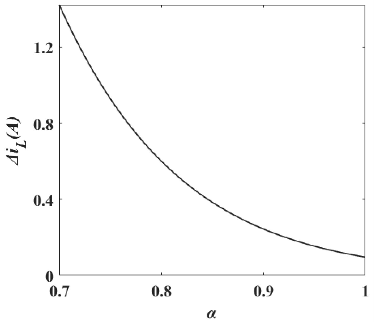
Equation (47) shows that when the fractional-order inductors L₁^α1 and L₂^α2 have equal inductance values and orders, the inductor current ripple is calculated by the same formula, and the inductor current ripple is related to its order. The curve of inductor current ripple Δi_L with order α can be obtained by using Matlab software, as shown in Figure 8. As the order decreases, the inductor current ripple Δi_L increases sharply, and the lower the order, the faster the ripple increases.

For a fractional-order Zeta converter to operate in CCM, the current flowing through the converter diode S_D must always be greater than 0 in the $(n+D)T_S<t\le (n+1)T_S$ interval. In the $(n+D)T_S<t\le (n+1)T_S$ interval, the current flowing through the diode is equal to the sum of the two inductor currents.

$$i_{S_D}=i_{L1}+i_{L2}$$

(48)

The diode current i_D is always greater than 0. Equivalently, the DC component of the inductor current should always be greater than half of its current ripple amplitude, yielding the following expression:

$$(I_{L1}-\frac{1}{2}\Delta i_{L1})+(I_{L2}-\frac{1}{2}\Delta i_{L2})>0$$

(49)

Substituting Equation (46) into Equation (49) and simplifying it can be expressed in the following form:

$$(I_{L1}+I_{L2})-\frac{V_{in}}{2}[\frac{{(DT)}^{{\alpha }_1}}{L_1{\alpha }_1\Gamma ({\alpha }_1)}+\frac{{(DT)}^{{\alpha }_2}}{L_2{\alpha }_2\Gamma ({\alpha }_2)}]>0$$

(50)

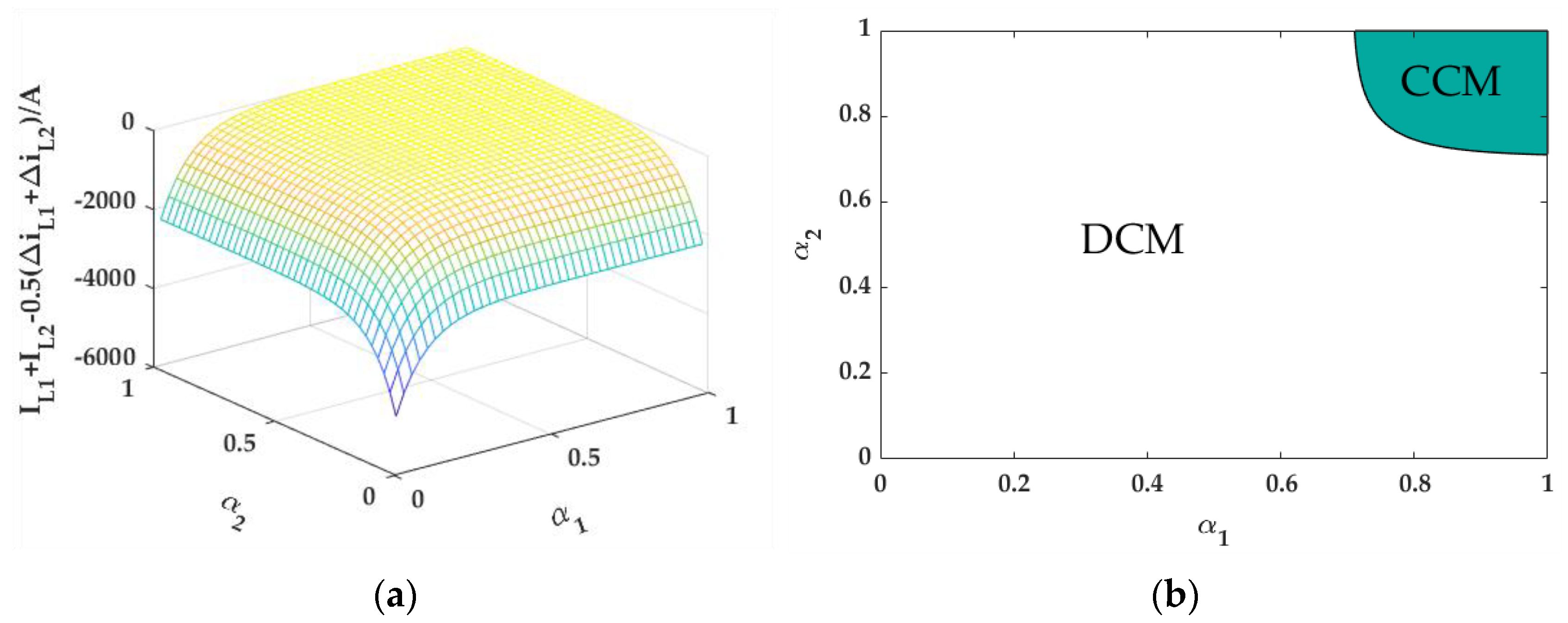
The effect of order α₁ and α₂ of the fractional-order inductor on the converter operation mode can be obtained from Equation (50), as shown in Figure 9.

Figure 9a shows the three-dimensional diagram of the current relative to the order α₁-α₂ plane change of Equation (50). When this current is greater than 0, it indicates that the converter is operating in CCM mode; when this current is less than 0, it indicates that the converter is operating in DCM mode; when this current is equal to 0, it indicates that it is operating in the critical state of CCM and DCM; the boundary lines of the two operating modes are shown in Figure 9b. From Figure 9b, the intersection coordinates (0.71, 1) and (1, 0.71) of the dividing line and the edge of α₁-α₂ plane can be obtained. Only when the inductance order is greater than 0.71 order can the converter run in CCM mode.

5. Analysis of Harmonic Components in Different Orders

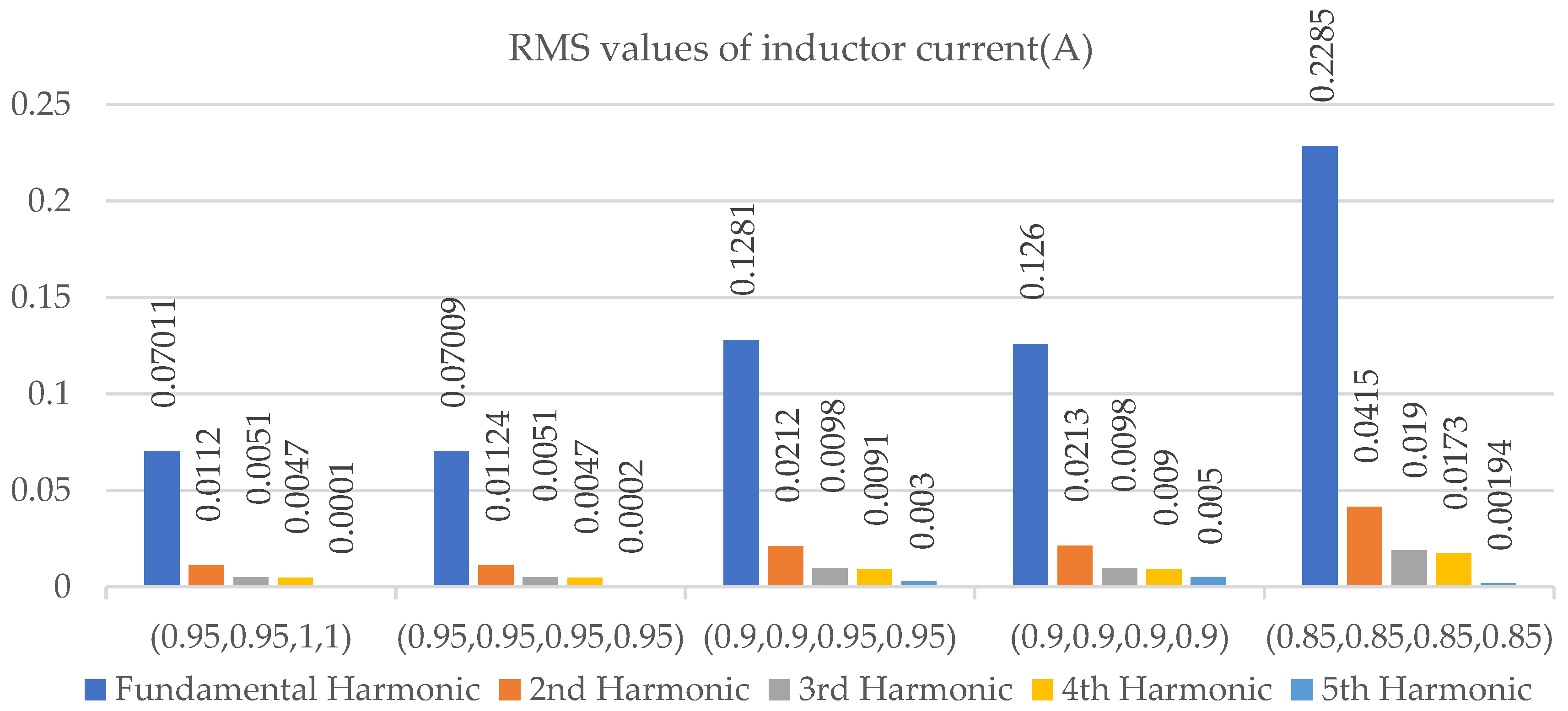
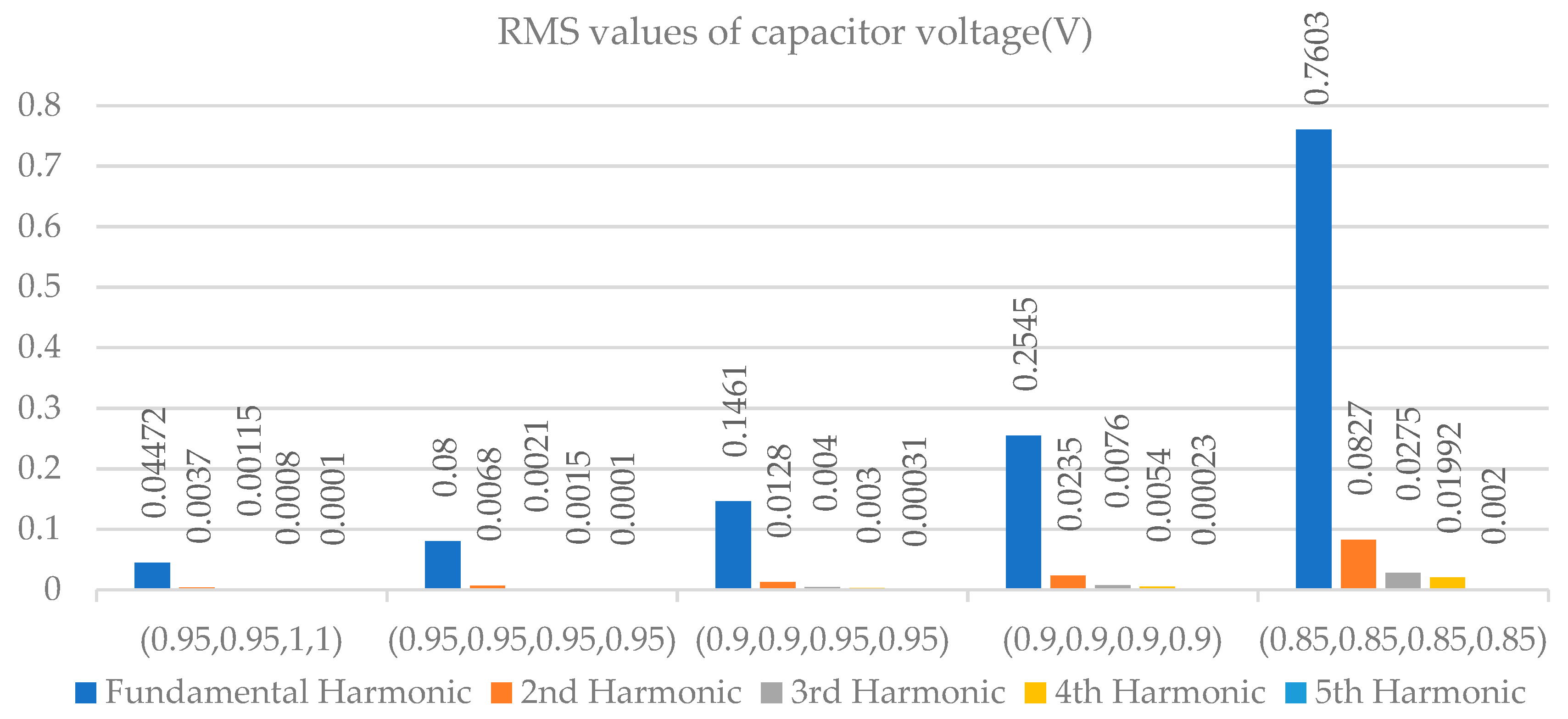
The steady-state approximate analytical solution of the fractional-order CCM Zeta converter is obtained through the analytical modeling method in Section 2. It is observed that both the DC component and the ripple of the energy storage element are related to the order of the energy storage element in the study. The specific change rule is as follows: when the order of the energy storage element decreases, the ripple amplitude of the state variable increases; in the contrary, the ripple amplitude of the state variable decreases. When the inductor and capacitor are in different orders, the harmonic amplitudes of the converter inductor current and capacitor voltage are obtained, as shown in Figure 10 and Figure 11, respectively.

From Figure 10 and Figure 11, as the order of the inductor and capacitor elements decreases, the amplitudes of the fundamental, second, third, fourth, and fifth harmonics of the inductor current and capacitor voltage increase. Since the ripple of the state variable is jointly affected by the harmonics, the changing trend of the harmonics in the state variable is consistent with the changing trend of the ripple amplitude. The change in the inductance order greatly influences the inductor current, while the change in the capacitance order has a relatively small influence on the inductor current.

The modified termination criterion of the analytical solution proposed in Equation (21) is verified by the change in each harmonic amplitude. The condition of the discriminant stability were analyzed with respect to the harmonic components. The effective values of the harmonic components of the converter inductor current and capacitor voltage, as a percentage of the fundamental component, were obtained, as shown in Figure 12. As can be seen from Figure 12, the value of the modified termination discriminant condition increases as the fractional order of the inductor and capacitor decreases.

6. Conclusions

Based on the extended harmonic balance principle and the idea of disturbance, ESPM was used to model the fractional CCM zeta converter. The steady-state analytical expression was obtained. According to the steady-state analytical expression, the fractional-order CCM Zeta converter was modeled in MATLAB and compared with the Oustaloup’s filter-based approximation method. Furthermore, the harmonic amplitude of each order of the state variables of the fractional CCM Zeta converter was obtained, and the influence of the order of the energy storage element on the harmonic components of each order was analyzed. The obtained results show that:

(1)

ESPM can avoid the discussion of the applicability of several fractional calculus definitions to the upper and lower limits of the integration under different circumstances, and overcome the problem that it is difficult for the fractional system to obtain specific expressions. The obtained solutions conclude practical physical significance, and the analysis results are consistent with those obtained by the Oustaloup’s filter-based approximation method.

(2)

The amplitude of each harmonic of the fractional converter is related to the order of the inductance and capacitance components. With all other parameters unchanged, when the fractional order of inductance and capacitance decreases, the amplitude of the harmonic components of each order in the state variable increases, increasing the amplitude of the inductor current and capacitance voltage ripple of the fractional order converter.

(3)

Compared with the numerical simulation method, the proposed method can better describe the change in the state variable ripple. The computational complexity is significantly reduced, the simulation speed is fast, and the memory consumption is small.

The ESPM is a fast algorithm for solving the steady-state periodic solution of Zeta circuits. The algorithm is a symbolic algorithm which overcomes the drawback of too many variable symbols in similar symbolic algorithms and uses matrix operations to make the whole solution process intuitive and clear. However, the equivalent small parameter method also has some problems; for example, the modeling of a high-order converter is complicated, and the converter with low-order-of-energy storage components needs to derive the high-order correction. This paper uses ESPM to model and analyze the fractional-order Zeta converter in CCM mode, and deduces the boundary conditions of the CCM mode and DCM mode. The modeling method proposed in this paper can be easily extended and applied to the fractional-order Zeta converter in DCM mode and other converter circuits.

References

- Jonscher, A.K. Dielectric Relaxation in Solids, Chelsea; Dielectrics Pub.: London, UK, 1983. [Google Scholar]
- Westerlund, S. Causal Consulting: Dead Matter Has Memory; Casual Consulting: Kalmar, Sweden, 2002. [Google Scholar]
- Chen, X. Research on Analytical Modeling Methods and Nonlinear Dynamic Characteristics of Fractional-Order DC/DC Converters. Ph.D. Thesis, South China University of Technology, Guangzhou, China, 2018. [Google Scholar]
- Kianpoor, N.; Yousefi, M.; Bayati, N. Fractional Order Modelling of DC-DC Boost Converters. In Proceedings of the 2019 IEEE 28th International Symposium on Industrial Electronics (ISIE), Vancouver, BC, Canada, 12–14 June 2019. [Google Scholar]
- Tan, C.; Liang, Z.S. Fractional order modeling and analysis of Boost converter in inductor current pseudo-continuous mode. Acta Phys. Sin. 2017, 63, 58–67. [Google Scholar]
- Yang, R.C.; Liao, X.Z. Modeling and analysis of fractional order Buck converter using Caputo–Fabrizio derivative. Energy Rep. 2020, 6, 440–445. [Google Scholar] [CrossRef]
- Wang, F.; Ma, X.K. Modeling and analysis of the fractional order buck converter in DCM operation by using fractional calculus and the circuit-Averaging Technique. J. Power Electron. 2013, 13, 1008–1015. [Google Scholar] [CrossRef]
- Wei, Z.H.; Zhang, B.; Jiang, Y.W. Analysis and Modeling of Fractional-Order Buck Converter Based on Riemann-Liouville Derivative. IEEE Access 2019, 7, 162768–162777. [Google Scholar] [CrossRef]
- Xie, L.L.; Liu, Z.P.; Zhang, B. A Modeling and Analysis Method for CCM Fractional Order Buck-Boost Converter by Using R–L Fractional Definition. J. Electr. Eng. Technol. 2020, 15, 1651–1661. [Google Scholar] [CrossRef]
- Xie, L.L.; Liu, Z.P.; Ning, K.Z. Fractional-Order Adaptive Sliding Mode Control for Fractional-Order Buck-Boost Converters. J. Electr. Eng. Technol. 2022, 17, 1693–1704. [Google Scholar] [CrossRef]
- Sarwar, S. On the Existence and Stability of Variable Order Caputo Type Fractional Differential Equations. Fractal Fract. 2022, 6, 51. [Google Scholar] [CrossRef]
- Wang, Z.Q.; Cao, J.Y. Numerical Solution of Fractional-Order Differential Integration Equations and Their Error Analysis; Xi’an Jiaotong University Press: Xi’an, China, 2015. [Google Scholar]
- Chen, X.; Chen, Y.F.; Zhang, B. A Modeling and Analysis Method for Fractional-Order DC-DC Converters. IEEE Trans. Power Electron. 2017, 32, 7034–7044. [Google Scholar] [CrossRef]
- Chen, Y.F.; Chen, X.; Hu, J. A symbolic analysis method for fractional-order boost converter in discontinuous conduction mode. In Proceedings of the IECON 2017—43rd Annual Conference of the IEEE Industrial Electronics Society, Beijing, China, 29 October–1 November 2017; IEEE: New York, NY, USA, 2017. [Google Scholar]
- Xu, J.; Li, X.; Liu, H. Fractional-Order Modeling and Analysis of a Three-Phase Voltage Source PWM Rectifier. IEEE Access 2020, 8, 13507–13515. [Google Scholar] [CrossRef]
- Sharma, M.; Rajpurohit, B.S.; Agnihotri, S.; Rathore, A.K. Development of Fractional Order Modeling of Voltage Source Converters. IEEE Access 2020, 8, 142652–142662. [Google Scholar] [CrossRef]
- Chen, B.; Li, C.; Wilson, B.; Huang, Y. Fractional modeling and analysis of coupled MR damping system. IEEE/CAA J. Autom. Sin. 2016, 3, 288–294. [Google Scholar]
- Chen, Y.F.; Xiao, W.X.; Zhang, B. Nonlinear Modeling and Harmonic Analysis of Magnetic Resonant WPT System Based on Equivalent Small Parameter Method. IEEE Trans. Ind. Electron. 2019, 66, 6604–6612. [Google Scholar] [CrossRef]
- Tseng, C.-C.; Lee, S.-L. Computation of fractional derivatives using Fourier transform and digital FIR differentiator. Signal Process. 2000, 80, 151–159. [Google Scholar] [CrossRef]
- Mohamed, A.; Rachid, M. Numerical Simulations of Fractional Systems: An Overview of Existing Methods and Improvements. Nonlinear Dyn. 2004, 38, 117–131. [Google Scholar]
- Xie, L.L.; Ning, K.Z.; Qin, L. Fractional Order Modeling and Simulation Analysis of Cuk Converter. Comput. Simul. 2022, 39, 313–320. [Google Scholar]
Figure 1.
Fractional-order Zeta converter.
Figure 2.
Working mode 1 of fractional-order CCM-Zeta converter.
Figure 3.
Working mode 2 of fractional-order CCM-Zeta converter.
Figure 4.
Simulation model of fractional-order CCM Zeta converter.
Figure 5.
Equivalent circuit of fractional element. (a) Fractional-order inductor; (b) fractional-order capacitor.
Figure 6.
Inductance current waveform of different orders: (a) (α1, α2, β1, β2) = (1, 1, 1, 1); (b) (α1, α2, β1, β2) = (0.95, 0.95, 1, 1); (c) (α1, α2, β1, β2) = (0.95, 0.95, 0.95, 0.95); (d) (α1, α2, β1, β2) = (0.9, 0.9, 0.95, 0.95); (e) (α1, α2, β1, β2) = (0.9, 0.9, 0.9, 0.9); (f) (α1, α2, β1, β2) = (0.85, 0.85, 0.85, 0.85).
Figure 7.
Capacitance voltage waveform of different orders: (a) (α1, α2, β1, β2) = (1, 1, 1, 1); (b) (α1, α2, β1, β2) = (0.95, 0.95, 1, 1); (c) (α1, α2, β1, β2) = (0.95, 0.95, 0.95, 0.95); (d) (α1, α2, β1, β2) = (0.9, 0.9, 0.95, 0.95); (e) (α1, α2, β1, β2) = (0.9, 0.9, 0.9, 0.9); (f) (α1, α2, β1, β2) = (0.85, 0.85, 0.85, 0.85).
Figure 8.
The relationship between inductance current ripple and inductance order.
Figure 9.
Influence of inductor order on operation mode of the converter. (a) Three-dimensional graph. (b) Boundary between CCM and DCM.
Figure 10.
Harmonic components of inductor currents with different orders in the CCM region.
Figure 11.
Harmonic components of capacitor voltages with different orders in the CCM region.
Figure 12.
Change in effective value of harmonic component in converter state variable with order.