A Comparative Study of the Kalman Filter and the LSTM Network for the Remaining Useful Life Prediction of SOFC

Abstract

The solid oxide fuel cell (SOFC) system is complicated because the characteristics of gas, heat, and electricity are intricately coupled. During the operation of the system, problems such as frequent failures and a decrease in the stack’s performance have caused the SOFC system to work less well and greatly shortened the SOFC’s practical life. As such, it is essential to accurately forecast its remaining useful life (RUL) to make the system last longer and cut down on economic losses. In this study, both model-based and data-driven prediction methods are used to make predictions about the RUL of SOFC. First, the linear degradation model of the SOFC system is established by introducing degradation resistance as the index of health status. Using the Kalman filtering (KF) method, the health status of SOFC is evaluated online. The results of the health state estimation indicated that the KF algorithm is accurate enough to provide a good basis for the model-based RUL prediction. Then, a long short-term memory (LSTM) network-recursive (data-driven) method is presented for RUL prognostics. The multi-step-ahead recursive strategy of updating the network state with actual test data improves the prediction accuracy. Finally, a comparison is made between the LSTM network prediction approach suggested and the model-based KF prognostics. The results of the experiments indicate that the LSTM network is more suitable for RUL prediction than the KF algorithm.

1. Introduction

The solid oxide fuel cell (SOFC) is used in many scenarios because of its near-zero pollution, high power density, fuel adaptability, and high efficiency [1,2]. However, performance degradation or even failure in actual operation makes SOFC systems poor in durability, which inhibits their widespread commercialization. The SOFC system is complicated, with multiple physical (electrochemical, thermodynamic, mechanical, fluidic), spatial, and temporal scales [3]. The precise degradation mechanism of the stack is still not fully understood. Moreover, the stack’s performance is significantly impacted by the frequent fluctuations in operating conditions [4,5,6]. In addition, some other failures, such as carbon deposition, chromium poisoning, and deterioration of BOP (balance of plant) elements, will also contribute to the short service life of the SOFC system [7]. To guarantee the safety and stability of the system, the development of prognostics and health management (PHM) techniques has received considerable attention. As the key of PHM, the remaining useful life (RUL) prediction is fascinating. Its goal is to check on the health of the SOFC and figure out how long it has left before it breaks down [8]. Therefore, even though material deterioration is unavoidable, a precise prediction can help people take steps early on to slow down the process [9], thus maximizing the system’s availability and reducing operating costs.

Much effort has been put into RUL prediction from various fields, such as mechanical systems (e.g., bearings) and electrochemical ones (e.g., batteries, proton exchange membrane fuel cells (PEMFCs)). However, little work has been done for the SOFC RUL. This makes it meaningful to screen the main ideas of other research objects for potential use in SOFC. In general, the prognostic approaches for RUL prediction can be put into one of the following three groups: model-based, data-driven, or hybrid [10]. The hybrid prognostics method, because it can combine the advantages of various methods and compensate for each other’s deficiencies, has gradually become the focus of current RUL forecasting research. Ge et al. [11] reviewed the hybrid RUL prediction of lithium batteries. Most hybrid approaches either integrate several data-driven methods or combine model-based and data-driven methods. Liu et al. [12] came up with a strategy for predicting RUL for aircraft auxiliary power units (APU), which merged an artificial intelligence-based model with a physics-based model. The experimental findings show that this approach can improve the precision and stability of RUL prediction not only for the aircraft APU but also for other complex systems. A fusion prognosis technique based on a long short-term memory (LSTM) network and a particle filter (PF) was reported by Xie et al. [13]. The results of the experiments demonstrated that it could produce better prognostic performance than a single prediction method. Some new forecasting problems are well solved with the hybrid approaches described above, but it is essential to comprehend the characteristics of a single method first. Simultaneously, figuring out how to combine them and change the parameters is also challenging.

The model-based approach aims to set up a model that matches how the system degrades over its entire life cycle so that the RUL can be predicted. Model-based methods require fewer data and directly reflect the fuel cell’s decay process, making them more practical [14]. Electrochemical models, equivalent circuit models (ECMs), and empirical models are common deterioration models [15]. Lyu et al. [16] showed a method for predicting the RUL of lead–acid batteries that uses a PF method combined with an electrochemical model. However, since fuel cell degradation is a complex, unobservable problem, it is usually hard to make a precise physical degradation model, particularly when the stack operates in unknown surroundings. Gallo et al. [17] reported a diagnostic approach integrating electrochemical impedance spectroscopy (EIS) with model-based aging estimation for SOFC RUL prediction. A stack aging model was developed by merging similar features from ECM parameters to simulate fuel cell degradation. The parameters of the fuel cell ECMs are often estimated utilizing EIS measurements [18]. However, EIS needs extra equipment to be measured, and the cost of the measurement is quite high. The empirical model is simpler to build and adaptable to a wider variety of scenarios than the other two models [19]. Chen et al. [20] constructed an empirical voltage degradation model for fuel cells. Using this model and the unscented Kalman filter (UKF) method, they predicted the degradation trend well. The limitation is that the measured voltage is selected as the degradation indicator. It is widely known that the system’s working environment significantly impacts the output voltage. Therefore, it becomes difficult to tell if the voltage decrease is due to the stack’s deterioration, the workload alteration, or if it is a response of the system due to the controller [21]. To improve the prognostics accuracy, Dolenc et al. [22] introduced area-specific resistance (ASR) as a health indicator to estimate the RUL, and a linear Kalman filter (KF) was employed to identify the parameters used in the empirical model.

With the significant increase in the computing capacity of computers, data-driven methods have steadily become the focus of RUL prediction research. The goal of data-driven methods is to investigate the potential association between sensor measurement data and the RUL value based on previous data [23]. However, the accuracy of the data-based algorithms mainly depends on the constructed mapping relationships that are sensitive to historical data [24]; in other words, when the quantity or quality of historical data is insufficient, data-driven methods may not achieve the expected results. However, this type of method does not require any prior knowledge of the system’s degradation mechanism or the creation of a reliable degradation model [25]. It is easy to implement and has excellent predictive power with the help of superior machine learning techniques. Javed et al. [26] put forward a summation-wavelet extreme learning machine (SW-ELM) model to estimate the RUL of PEMFC. Experimental results demonstrate the adaptability of this approach with limited data. Support vector machine (SVM), as a typical representative of the machine learning algorithm, is widely used in RUL prediction [27]. The performance of the SOFC stack was forecasted via three algorithms by Song et al. [28]. The comparison results indicated that the neural network (NN) prediction effect is better than the machine learning (SVM). The LSTM network [29] is a particular type of recurrent neural network (RNN). By incorporating a sigmoid layer known as the forget gate layer, the LSTM network is able to avoid the problems that traditional RNNs have with gradient disappearance and explosion [30]. The application of the LSTM network in the RUL estimation of lithium batteries [31] and turbofan engines [32] proves its potential for time sequence prediction. Liu et al. [33] employed an LSTM-RNN approach to deal with the PEMFC degradation issue. The fuel cell RUL was predicted quickly and accurately. However, the prediction was made only one step ahead, which is insufficient for most practical uses.

Each research approach has its own strengths and weaknesses and can be more or less useful depending on the circumstances. In general, RUL prediction has gotten a lot of attention from many various fields, and there have been many research findings. However, prognostication of SOFCs, the process that comes after monitoring and diagnostics, is still a young field of scientific investigation [34]. There have been relatively few studies conducted in the area of RUL prediction for SOFCs [17]. To close this gap, both model-based and data-driven prediction methods are used to figure out the RUL of SOFC. These methods take into account the characteristics of SOFC, and the existing available data [35] provide an essential basis for verifying the methods. The primary contributions to this work are as follows:

(1)

The Kalman filtering (KF) and LSTM networks are used to predict the RUL of SOFC, respectively. Moreover, the prediction effects are compared and analyzed in detail.

(2)

The linear degradation model of the SOFC system is established by taking the degradation resistance as the health index, and the accurate KF estimation provides a good foundation for predicting SOFC RUL.

(3)

The multi-step-ahead recursive strategy of updating the network state with actual test data improves prediction accuracy, enhancing the practical application value.

The following describes the arrangement of this paper: In Section 2, the experiment configurations and data preparation are illustrated; in Section 3, two RUL prediction methods for fuel cells are presented; and the analysis and comparison of the RUL prediction results using the above two methods are displayed in Section 4. The conclusion is in Section 5.

2. Experimental Configurations and Data Acquisition

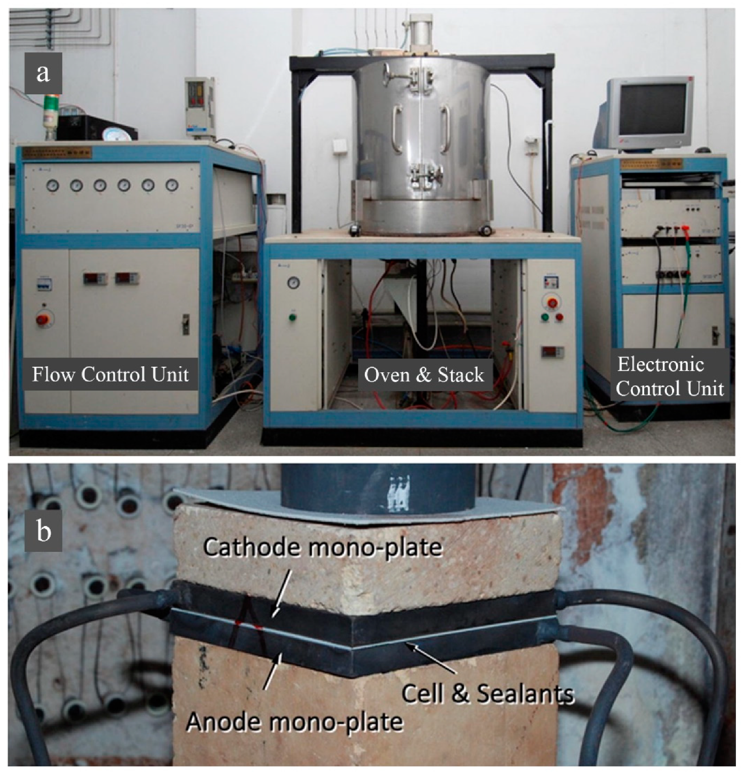
2.1. Experimental Platform

Prior to estimating the RUL of a SOFC stack, the stack’s durability test should be carried out first. As given in Figure 1a, this paper developed an independent SOFC test bench in the Fuel Cell Research Center of Huazhong University of Science and Technology [35]. The stack is installed in the oven. The anode reductant of the stack is hydrogen, and the cathode oxidizer is dehumidified air.

The investigated stack adopts a single anode-supported SOFC, as depicted in Figure 1b. The cell’s dimensions are 11 cm × 11 cm × 1 mm, and its cathode-active area is 9 cm × 9 cm. The anode-supported material is Ni–YSZ (Yttria Stabilized Zirconia).

Table 1. Experimental configuration.

Parameter	Value	Parameter	Value
Related to fuel cell
Thickness of YSZ electrolyte	10 μm	Thickness of anode functional layer	10 μm
Thickness of anode support	1 mm	Thickness of YSZ-based cathode	≤3 μm
Related to operating conditions
Stack temperature	750 °C	Air flow rate	2 NL/min
Hydrogen flow rate	2 NL/min	Load current	0.37 A/cm2 (30 A)

briefly overviews the fuel cell [35], including the materials for other composition sections. More specific details about the fuel cell manufacturing method can be found in Ref. [36].

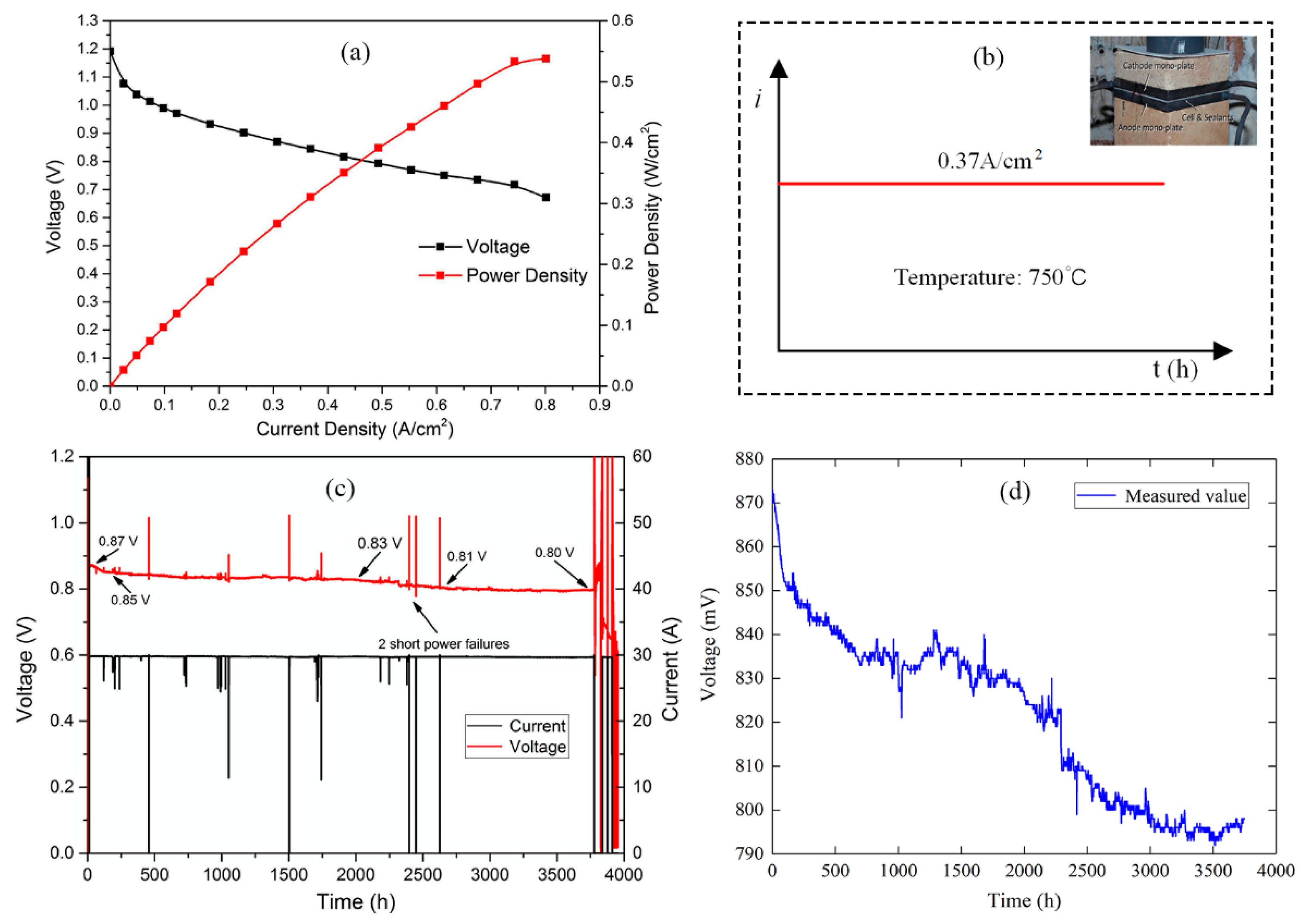
2.2. Experimental Data Acquisition

In the anode atmosphere of 5% H₂ + N₂, the stack was heated to a stable temperature of 750 °C [35]. Following the stabilization of the open circuit voltage (OCV), the i-v curve (Figure 2a) was plotted by discharging the stack at different currents to see how well it worked, after which it was subjected to a constant discharge current to assess the stack’s durability, as shown in Figure 2b.

Figure 2c displays the stack deterioration curve under steady-state operation conditions (750 °C and 0.37 A/cm²). The testing was carried out for close to 4000 h. The original voltage rose from 0.86 V to 0.87 V in 120 h before falling to 0.85 V. Over the next 1800 h, the voltage dropped steadily to 0.83 V. At the 2500th hour, the voltage decreased relatively quickly, eventually reaching around 0.81 V. After that, the fuel cell stack voltage stabilized at 0.8 V. The test experiment was interrupted after an unexpected external power failure occurred in the 3770th hour. During this time, the oven was forced to return to room temperature.

Some interferences, such as electromagnetic interference, may lead to inaccurate calculations during the test. Moreover, too much data will cost much computing time, so it is necessary to preprocess the original data. By setting the sampling period to 1 h and removing the out-of-range values that changed a lot by hand, a 3750-h data set was finally selected for subsequent health assessment and life prediction. Figure 2d shows the voltage data after pretreatment. The voltage in the 3750th hour is around 798 mV. It can be seen from the figure that the processed data not only retains the primary trend of the original information but also effectively removes noise and spikes.

3. RUL Prediction Methods

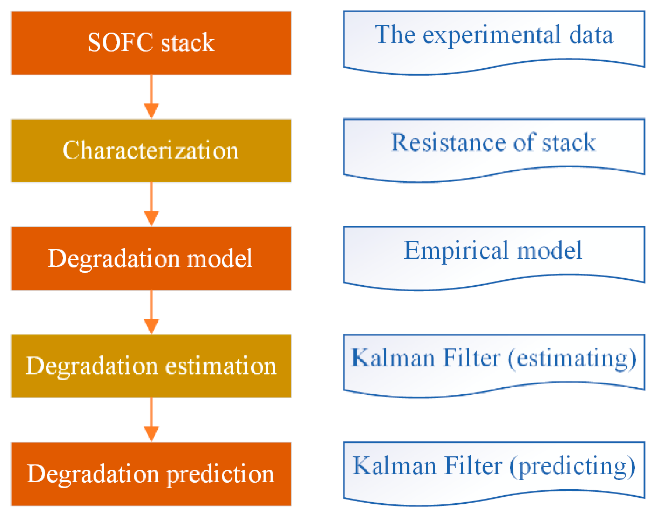
3.1. The Model-Based RUL Prediction Method

For the model-based RUL prediction, the system’s degradation law or failure mechanism is used to build a matching physical model. Then, RUL forecasting can be performed with the physical model. This method is very applicable to research items with clear degradation mechanisms, and the degradation model can correspond to physical quantities one by one, which has strong interpretability. The model-based RUL prediction processes are presented in Figure 3, which are as follows: Choose a degradation index; model the degradation process; estimate the health state; forecast RUL; and evaluate performance.

3.1.1. SOFC Degradation Model

The SoH (state of health) of SOFC is a crucial performance parameter used to characterize the degree of its performance deterioration. The most common way to choose health indicators is to use the voltage as a status indicator and calculate the remaining life when the stack voltage obviously drifts. However, the stack voltage is extremely sensitive to operational conditions. For the performance prediction to work well in real operating conditions, there needs to be an appropriate indicator.

The internal resistance is a result of many chemical reactions happening simultaneously on the stack, and it carries crucial information about the SoH of the stack. As described in the literature [21,37], they used area-specific resistance (ASR) as a health indicator. One of the benefits is that the ASR value of the fuel cell is invariant to the operating conditions of the system. It means that static operation is not necessary. On the other hand, it can weaken the voltage difference caused by various reactant components (CH₄, H₂, CO₂, CO, H₂O, and N₂) [37]. Therefore, this work chose degradation resistance as an index to evaluate SOFC health status.

In the state of SOFC performance degradation, its electrical characteristic equation can be written as follows [38]:

$$V_s=(E_{nernst}-V_{act}-V_{con}-V_{ohm})-I_s{R}_s$$

(1)

where V_s and I_s represent the output voltage and current, respectively. R_s is the lumped degradation resistance, indicating the SOFC resistance’s increased value as performance degrades. Nernst voltage E_nernst is calculated by the following equation [38]:

$$E_{nernst}=1.286-k_E(T_s-T_0)+\frac{R^{*}\cdot T_s}{2F}\ln \frac{P_{H_2}{P}_{O_2}^{0.5}}{P_{H_{2}O}}$$

(2)

where R* denotes the universal gas constant; F is Faraday’s constant; T_s indicates the stack temperature; and P_H2, P_O2, and P_H2O represent hydrogen, oxygen, and water vapor partial pressures inside the stack. The activation polarization voltage V_act can be expressed as [38]:

$$V_{act}=\frac{R^{*}\cdot T_s}{F}\left({\sinh }^{-1}\left(\frac{i_s}{2i_{0,a}}\right)+{\sinh }^{-1}\left(\frac{i_s}{2i_{0,c}}\right)\right)$$

(3)

where i_s denotes the current density; and i_0,a and i_0,c are the exchange current density of the anode and cathode, respectively. The concentration polarization loss V_con can be obtained by [38]:

$$V_{con}=\frac{R^{*}\cdot T_s}{n_{e}F}\ln \left(1-\frac{i_s}{2i_L}\right)$$

(4)

where i_L is the limit current density and n_e represents the number of free electrons. The ohmic polarization voltage V_ohm is computed as [38]:

$$V_{ohm}=i_s{T}_s{e}^{\frac{a_1}{T_s}+a_0}$$

(5)

where a₀ and a₁ are constants.

Table 2. Model parameters [38].

Parameter	Value	Parameter	Value
kE	2.304 × 10−4	T0	298.15 K
R*	8.314 J·mol·K−1	F	96,485 C·mol−1
iL	1 × 104 A·m−2	ne	2
I0,a	5300 A·m−2	io,c	2000 A·m−2
a0	−25.855	a1	7509.6

lists some parameters of the above formulas.

Because the SOFC degradation mechanism is unknown and constant thermodynamics are assumed, this paper uses the linear drift model below to describe the degradation process [21]. The model’s foundation is the idea that things should be as simple as possible and empirical analysis of experimental results.

$$R(t)={\alpha }_{k}t+b_k$$

(6)

where, ${\alpha }_k$ denotes the slope, $b_k$ indicates the intercept, and R(t) represents the ohmic resistance.

The Taylor series can be utilized to explain this linear model. The Taylor expansion is a common method for linearizing nonlinear functions, with the first two terms used to approximate the function. Thus, the trajectory of R(t) can be approximated and characterized by a linear function. The linearity of the drift model allows the KF algorithm to estimate its parameters with adequate precision.

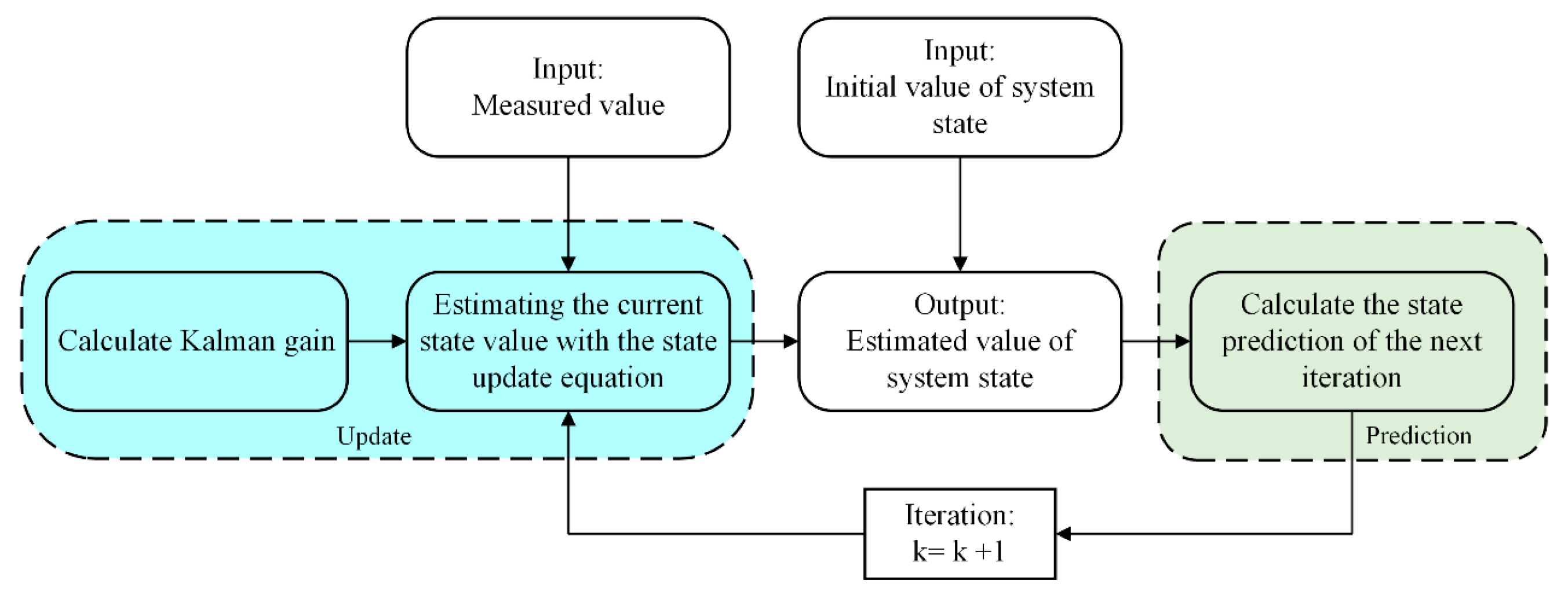
3.1.2. Health State Estimation Based on the Kalman Filter

This paper uses KF to predict the RUL of a single SOFC stack within a model-based framework. KF is a special optimal estimation algorithm, especially for linear systems. It determines the unbiased minimum variance of the system state based on input and output and integrates the state equation with the measurement equation [39]. The state equation expresses the change law of the state, but if only use the state equation, the error will not converge quickly. As such, to make the state estimation more accurate, it is vital to combine the measurement equation and use the measured data to correct the state error. The frame diagram of the KF recursive algorithm is described in Figure 4.

Firstly, convert the degradation model into a two-state discrete state space model [40]:

$$x_k=[\begin{array}{l}{R}_k\\ {\alpha }_k\end{array}]$$

(7)

x_k+1 = Ax_k + w_k

(8)

y_k = Hx_k + v_k

(9)

where x indicates the degradation state; α is the aging factor, also known as the gradient of a linear function; and the additional components w_k and v_k are both zero-expected white noise, and their covariances are the matrices L and M, respectively. A represents the state transition matrix for system degradation; y denotes the measurement output, which in this case is the resistance; and the matrix H relates the state to the measurement y_k.

$$A=\left[\begin{array}{cc}1& t_s\\ 0& 1\end{array}\right]$$

(10)

y_k = R_k

(11)

$$H=\left[\begin{array}{cc}1& 0\end{array}\right]$$

(12)

t_s denotes the sampling period, here t_s = 1 h. The following is the algorithm of the KF:

Initialization:

$$x_{0|0}=E(x_0)$$

(13)

$$P_{0|0}=Var(x_0)$$

(14)

Time update:

$${\widehat{x}}_{k|k-1}=A{\widehat{x}}_{k-1|k-1}$$

(15)

$$P_{k|k-1}=A{P}_{k-1|k-1}{A}^T+L$$

(16)

Measurement update:

$$K_k=P_{k|k-1}{H}_k^T{(H_k{P}_{k|k-1}{H}_k^T+M)}^{-1}$$

(17)

$${\widehat{x}}_{k|k}={\widehat{x}}_{k|k-1}+K_k(y_k-H_k{\widehat{x}}_{k|k-1})$$

(18)

$$P_{k|k}=(1-K_k{H}_k)P_{k|k-1}$$

(19)

Equations (15) and (16) represent time-based updates. Based on the optimally estimated value of the previous time ${\widehat{x}}_{k-1|k-1}$, the estimated value of the system’s current moment ${\widehat{x}}_{k|k-1}$ and the covariance of the system prediction error $P_{k|k-1}$ are obtained. $K_k$ is the Kalman gain. The measurement update equations in Formulas (18) and (19) update the current state prediction ${\widehat{x}}_{k|k-1}$. More details about the KF are given in Refs. [21,41].

It is challenging to obtain process noise and measurement noise in practice. To make the KF approach noise-tolerant and fast-convergent, after a series of parameter adjustments, L and M are set as:

$$L=\left[\begin{array}{cc}{10}^{-4}& 0\\ 0& {10}^{-12}\end{array}\right] \mathrm{and} M={10}^{-3}$$

(20)

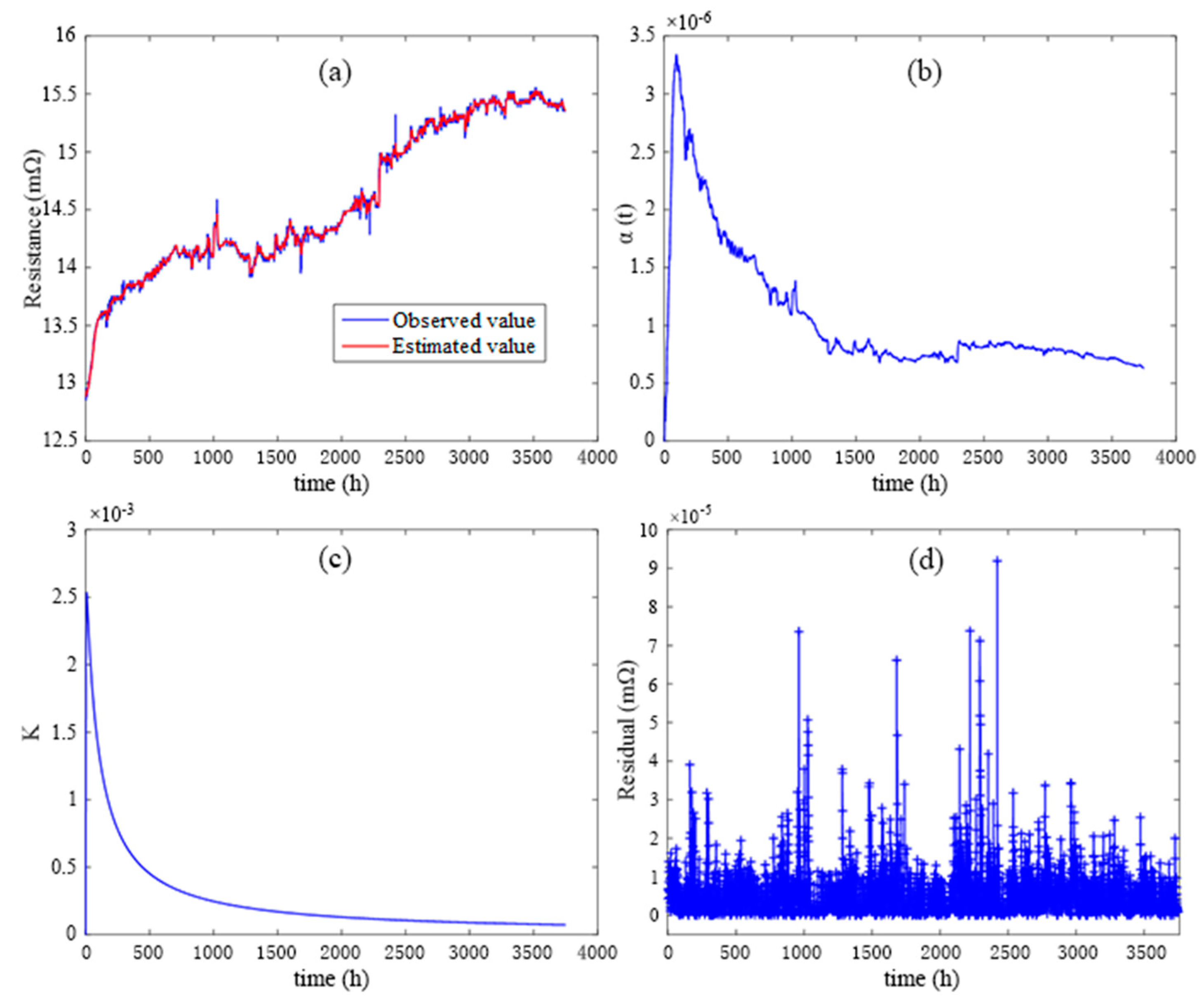
3.1.3. Estimation Results from the Kalman Filter

The results of health state estimation using the KF algorithm are displayed in Figure 5a. According to Figure 5a, the resistance value estimated by KF can track the measured one well. In most cases, the predicted value is very close to the observed value, except at specific peaks where the difference between the estimated and observed data is significant. In addition, the estimated value of degradation resistance includes time drift, which will be utilized to calculate RUL in the future. These verify the viability and effectiveness of modeling SOFC deterioration behavior as a linear model. In addition, as time passes, the stack further deteriorates, and the internal resistance grows. KF gives an accurate estimate of the degradation resistance of SOFC by eliminating oscillations caused by measurement noise while keeping the overall trend. Hence, we can say that using KF to estimate the model state is practical and accurate.

Figure 5b and c show the estimated values of the aging factor $\alpha (t)$ and Kalman gain K obtained by the KF algorithm, respectively. $\alpha (t)$ is the second state of the suggested KF, and the degradation rate increases quickly at first and then slowly decreases. The convergence of the KF algorithm can be judged by observing how the Kalman gain changes over time. It is evident from Figure 5c that the KF algorithm tends to converge when t = 3000 h. The residual result of the resistance is displayed in Figure 5d. The diagram illustrates that the maximum residual value is less than 10⁻⁴. This result indicates that the KF estimation is accurate enough to lay a good foundation for the following RUL prediction step.

3.2. The Data-Driven RUL Prediction Method

Within the framework of data-driven forecasting, we used the LSTM network method combined with a recursive strategy to make the RUL prediction. The scheme of the LSTM–Recursive prognostic approach is given in Figure 6. Details of the related contents will be shown below.

3.2.1. LSTM Network Model

As seen in Figure 6b, the LSTM has three layers: an input layer, a hidden layer, and an output layer. The most important thing about LSTM is that tiny linear interactions can change a cell from its previous state C_t−1 to its current state C_t [9]. The LSTM transmission state is determined by three gates, which can be expressed as three stages.

(1) The forgetting process. The first step is to determine which data the network needs to throw away or which data from the previous node it needs to forget. This is accomplished through the forget gate f_t, with the following calculation formula:

$$f_t=\sigma (W_f\cdot [h_{t-1},X_t]+b_f)$$

(21)

where σ denotes the activation function and in cell state C_t−1, the forget gate reads the previous step’s output h_t−1 and the current step’s input X_t. It then sends out a vector between [0, 1] that indicates which data is kept and which data is discarded.

(2) The selection/memory stage. At this stage, the input is selected and stored, and the input gate controls the information that has just been saved. The formulas for the calculation are as follows:

$$i_t=\sigma (W_i\cdot [h_{t-1},X_t]+b_i)$$

(22)

$${\tilde{C}}_t=\tanh (W_C\cdot [h_{t-1},X_t]+b_c)$$

(23)

where i_t is the input gate and ${\tilde{C}}_t$ indicates the updated value of the cell status. When data passes through the input gate, the internal state of the network needs to be updated. The update rule is to choose through the forget gate to throw away some of the last moment’s internal state information and then make a selection through the input gate so that new unit information C_t can be generated. The update process has the following mathematical form:

$$C_t=f_t\odot C_{t-1}+i_t\odot {\tilde{C}}_t$$

(24)

(3) The output stage. At this stage, the present state of the cell is evaluated by the output gate o_t, which then makes a decision on the cell’s output. The calculation formulas are shown below:

$$o_t=\sigma (W_o[h_{t-1},X_t]+b_o)$$

(25)

$$h_t=o_t\odot \tanh (C_t)$$

(26)

where the weights matrix is denoted by W_f, W_i, W_o, and W_c, while b_f, b_i, b_c, and b_o represent the deviation vectors, and $\odot$ indicates the element dot product.

In the output gate, the inputs X_t and h_t−1 are calculated by a sigmoid function to figure out whether or not the information can pass, so as to obtain the judgement condition. The tanh function takes the unit state C_t and turns it into a vector ranging from −1 to 1. This vector is then multiplied by the judgement condition to get the final output of the LSTM. More information about LSTM can be obtained in Ref. [13].

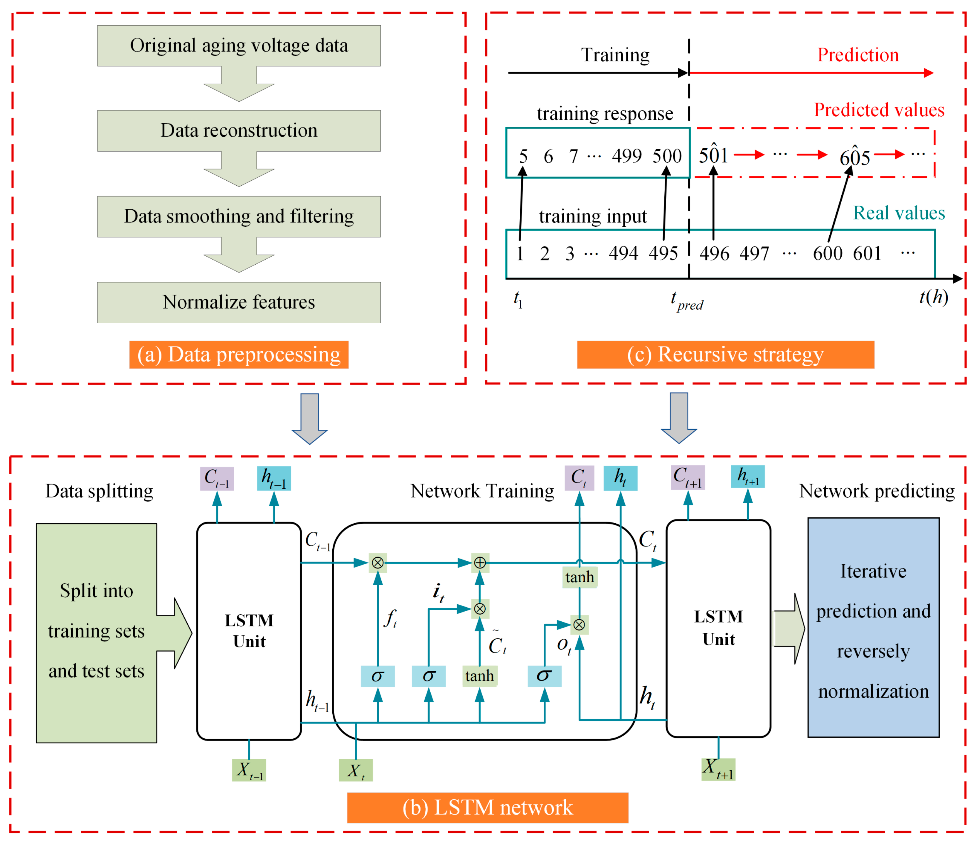
3.2.2. Prognostics Implementation with the LSTM-Recursive Method

As can be seen in Figure 6c, we used a recursive strategy to make the LSTM multi-step-ahead prediction. The distinctive property of this approach is that the accumulation of errors can be largely avoided by using the actual value instead of the estimated value of the previous step to conduct the prediction process.

The specific prognostics process with the LSTM–Recursive method is as follows:

(1)

Data standardization.

(2)

Data splitting. The voltage data was split into training sets and test sets.

(3)

Prepare training input and response. The response was designated as a new sequence formed by moving the values of the training sequence by four steps. In other words, at each time step of the input sequence, the LSTM network learns to predict the value of the following fourth-time step. Naturally, you can also move more steps to forecast the voltage situation at a further moment in the future.

(4)

Define the LSTM network structure and parameters. The specific values are given below.

(5)

Training the network. The “trainNetwork” library in MATLAB (MathWorks, R2021b) software trains the network using the training input and response.

(6)

LSTM prediction. Use the “resetState” function to reset the network state so that the predictions of the new data sets are not affected by the previous predictions. Then initialize the network state by predicting the training data. Further, use the “predictAndUpdateState” function to update the network status. The test data is used as the function’s input for each prediction, and the predicted stack voltage is the output. This process is iterative until the end of the test set traversal.

The code for the LSTM–Recursive prognostic model was completed in the script file built by MATLAB. The LSTM network parameters are configured as follows: the solver is set to ‘Adam’, and the network is trained for 250 epochs. The gradient threshold is set to 1 to prevent explosions of gradients. It starts with a learning rate of 0.005 and decreases by a factor of 0.2 after 125 rounds. The choice of an LSTM hidden unit is typically determined by engineering experience between 100 and 1000. In this work, 200 hidden cells are chosen to achieve the lowest possible error rate.

4. Results and Analyses

4.1. Performance Evaluation Criteria

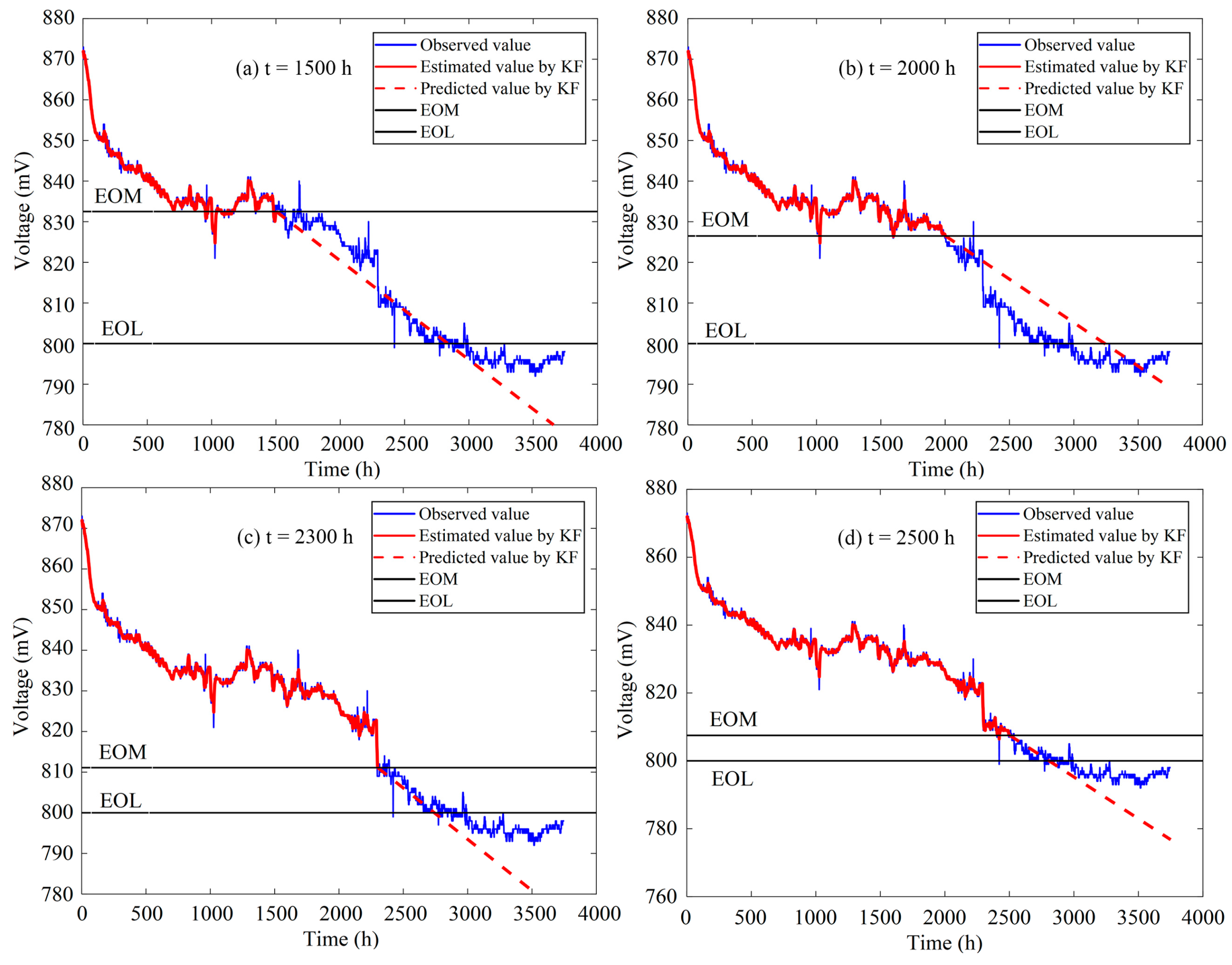
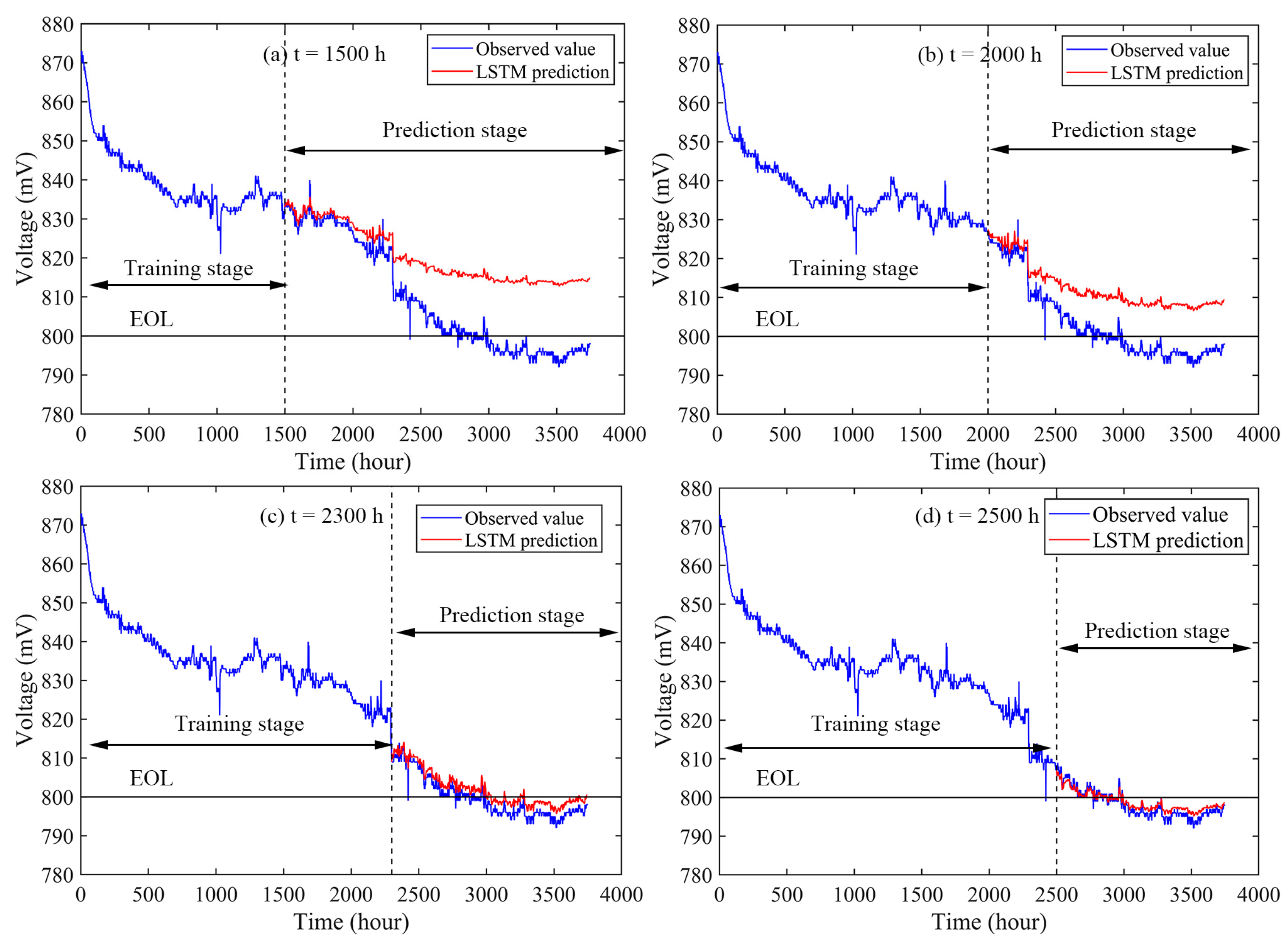
Root mean square error (RMSE) and mean absolute error (MAE), two statistical measures, are applied to judge the accuracy of predictions and compare how well the two forecasting approaches work. The smaller the two values, the more accurately the algorithm can forecast.

$$RMSE=\sqrt{\frac{1}{m}{\displaystyle \sum _{i=1}^m{(y_i-{\widehat{y}}_i)}^2}}$$

(27)

$$MAE=\frac{1}{m}{\displaystyle \sum _{i=1}^m\frac{\left|y_i-{\widehat{y}}_i\right|}{\left|y_i\right|}}$$

(28)

where m denotes the test data size, y_i represents the actual value, and ${\stackrel{}{\widehat{y}}}_i$ indicates the predicted result.

4.2. RUL Prediction

A system’s RUL is the time left until it fails, where failure means it cannot perform a specified function. Further, the prognostic process is split into two parts: the first is figuring out how healthy the system is right now and predicting how it will change until the preset failure threshold is achieved. Then, the RUL at time t RUL_pre(t) is determined by subtracting the time when the prognosis began from the anticipated end of life (EOL).

$$RU{L}_{pre}(t)=E_{pre}(t)-t$$

(29)

where E_pre(t) is the moment when the predicted results intersect with EOL. EOL can vary depending on the task and application, and its value can differ [21]. For example, drops in output voltage (e.g., should not exceed 10%) [26], power output (e.g., 4%) [42], or power conversion efficiency are all viable definitions of EOL. Here, the failure threshold EOL = 800 mV was selected (about a 9.2% drop from the initial voltage), which is reasonable and acceptable. t denotes the beginning point of life prediction, corresponding to the EOM (end of monitoring).

4.3. Analysis and Comparison of RUL Prediction Results

After determining that EOL is 800 mV, considering the uncertainty and a specific confidence interval, we can find that the real failure moment E_real(t) is approximately 2771 h. Combined with the training of data sets, t = 1500, 2000, 2300, and 2500 h are chosen as the starting points for a comprehensive evaluation of the prediction effect under different conditions. Figure 7 illustrates the RUL prediction results of the KF method. The red solid line in the first half of KF represents the KF state estimation result, while the red dashed line in the second half denotes the KF prediction result. The blue solid line throughout the entire period reflects the observed value. The EOM represents the prediction starting point, which means that from this point forward, the state parameters are fixed, and the RUL of the stack is predicted.

Since the filter cannot get the voltage observation data during the prediction stage, it is unable to correct the prior estimation, making it relatively hard to update. The prediction effect is a straight line, which cannot predict the local nonlinear change in voltage and track the voltage degradation trend well. The slope of the prediction straight line depends on the state estimation value of the prediction starting point.

Table 3. The RUL prediction results of the two approaches.

Method	Forecast Starting Point/h	RULreal/h	RULpre/h	RMSE	MAE
KF	1500	1271	1337	4.2324	0.0042
	2000	771	1241	7.3568	0.0078
	2300	471	441	1.7692	0.0018
	2500	271	307	1.7582	0.0018
LSTM	1500	1271	/	7.8885	0.0074
	2000	771	/	6.4721	0.0069
	2300	471	698	2.1802	0.0022
	2500	271	287	1.4373	0.0015

displays the specific performance criteria of the KF method. At t = 1500 h and t = 2000 h, the KF prediction effect is poor, with a significant prediction error. At t = 2300 h, the RMSE predicted by KF is 1.7692, and the MAE is 0.0018. The prediction effect of t = 2500 h is comparable to that of t = 2300 h, with an RMSE of 1.7582, slightly less than t = 2300 h, and an MAE of 0.0018, which is consistent with t = 2300 h. It can also be seen from the corresponding graph that when t = 2300 h and t = 2500 h, the slope of the prediction straight lines between EOM and EOL matches the linearity of the degraded data well.

In order to compare with the KF prediction results, the beginning points for the prediction have also been set at t = 1500, 2000, 2300, and 2500 h. The multi-step-ahead degradation prediction with LSTM is presented in Figure 8. In the figure, the blue line depicts the observed voltage, whereas the red line shows the predicted result. The first and second halves of the dotted line reflect the training and prediction stages, respectively. The figure shows that LSTM can well capture the trend of voltage degradation and predict the local nonlinear change of voltage. In addition, the observation was that the measurement data was effectively fitted in the early stage, but the prediction error increased somewhat as the prediction time increased. This finding suggests that the LSTM model may not have been overfitted to some extent.

Notably, when the prediction starting point is t = 1500, 2000, or 2300 h, the model’s predicted voltage value is slower than the actual one, its predicted voltage value is usually higher than the actual value, and the predicted voltage did not reach the failure threshold EOL before the moment of E_real(t). The later the starting point of prediction is, the more training data is used to train the model, and the more accurate the prediction effect will be. Specific performance indicators are also shown in Table 3. At t = 2500 h, the overall prediction curve matches the actual degradation trend well, and the overall prediction error is at its lowest, with RMSE = 1.4373 and MAE = 0.0015.

Comparing and analyzing the LSTM prediction results based on data with the KF prediction results based on the model, we can see that LSTM multi-step-ahead degradation prediction can capture the details of voltage deterioration and the overall degradation trend. Additionally, the later the prediction starting point, the more data is used for training, which will make the prediction more credible. However, the KF forecast accuracy mainly depends on the linearity of degradation data; it cannot track the local fluctuation and degradation trend of voltage. As such, we can say that the data-driven LSTM approach is more suitable for RUL estimation than the KF approach.

5. Conclusions

This paper presents two prognostic methods for RUL prediction of SOFC. In order to verify the effectiveness of the proposed methods, the aging data sets were obtained from an experimental platform built by our laboratory. For the model-based KF method, a linear deterioration model uses degradation resistance as an indicator of SOFC health status. The degradation estimation is then implemented to check the health status of SOFC online. The maximum residual value of the resistance is less than 10⁻⁴ indicates that the KF estimation is accurate enough to lay a good foundation for predicting SOFC RUL. The KF prediction results suggest that it can only predict the short-term degradation trend, and the forecast accuracy mainly depends on the linearity of degradation data. For the data-driven (LSTM network–Recursive) method, the multi-step-ahead recursive strategy of updating the network state with test data increases the prediction accuracy. The RUL forecasting outcomes show that the suggested LSTM technique can capture the details of voltage deterioration and make the prediction more credible with more training data. The comparison results of the two approaches reveal that the LSTM network is more suitable for RUL prediction than the KF algorithm. Currently, the SOFC RUL prediction verification under stable operating conditions has been implemented. Future work will improve the prediction’s generalization ability while operating under a dynamic load.

References

1. Yang, B.; Wang, J.; Zhang, M.; Shu, H.; Yu, T.; Zhang, X.; Yao, W.; Sun, L. A state-of-the-art survey of solid oxide fuel cell parameter identification: Modelling, methodology, and perspectives. Energy Convers. Manag. 2020, 213, 112856. [Google Scholar] [CrossRef]
2. Xu, H.; Ma, J.; Tan, P.; Chen, B.; Wu, Z.; Zhang, Y.; Wang, H.; Xuan, J.; Ni, M. Towards online optimisation of solid oxide fuel cell performance: Combining deep learning with multi-physics simulation. Energy AI 2020, 1, 100003. [Google Scholar] [CrossRef]
3. Jiang, H.; Xu, L.; Struchtrup, H.; Li, J.; Gan, Q.; Xu, X.; Hu, Z.; Ouyang, M. Modeling of Fuel Cell Cold Start and Dimension Reduction Simplification Method. J. Electrochem. Soc. 2020, 167, 044501. [Google Scholar] [CrossRef]
4. Zheng, Y.; Wu, X.-l.; Zhao, D.; Xu, Y.-w.; Wang, B.; Zu, Y.; Li, D.; Jiang, J.; Jiang, C.; Fu, X.; et al. Data-driven fault diagnosis method for the safe and stable operation of solid oxide fuel cells system. J. Power Sources 2021, 490, 229561. [Google Scholar] [CrossRef]
5. Cuneo, A.; Zaccaria, V.; Tucker, D.; Traverso, A. Probabilistic analysis of a fuel cell degradation model for solid oxide fuel cell and gas turbine hybrid systems. Energy 2017, 141, 2277–2287. [Google Scholar] [CrossRef]
6. Zeng, Z.; Qian, Y.; Zhang, Y.; Hao, C.; Dan, D.; Zhuge, W. A review of heat transfer and thermal management methods for temperature gradient reduction in solid oxide fuel cell (SOFC) stacks. Appl. Energy 2020, 280, 115899. [Google Scholar] [CrossRef]
7. Peng, J.; Huang, J.; Wu, X.-L.; Xu, Y.-W.; Chen, H.; Li, X. Solid oxide fuel cell (SOFC) performance evaluation, fault diagnosis and health control: A review. J. Power Sources 2021, 505, 230058. [Google Scholar] [CrossRef]
8. Wu, X.; Ye, Q.; Wang, J. A hybrid prognostic model applied to SOFC prognostics. Int. J. Hydrogen Energy 2017, 42, 25008–25020. [Google Scholar] [CrossRef]
9. Zhang, Z.; Wang, Y.-X.; He, H.; Sun, F. A short- and long-term prognostic associating with remaining useful life estimation for proton exchange membrane fuel cell. Appl. Energy 2021, 304, 117841. [Google Scholar] [CrossRef]
10. Rao, M.; Wang, L.; Chen, C.; Xiong, K.; Li, M.; Chen, Z.; Dong, J.; Xu, J.; Li, X. Data-Driven State Prediction and Analysis of SOFC System Based on Deep Learning Method. Energies 2022, 15, 3099. [Google Scholar] [CrossRef]
11. Ge, M.-F.; Liu, Y.; Jiang, X.; Liu, J. A review on state of health estimations and remaining useful life prognostics of lithium-ion batteries. Measurement 2021, 174, 109057. [Google Scholar] [CrossRef]
12. Liu, X.; Liu, L.; Liu, D.; Wang, L.; Guo, Q.; Peng, X. A Hybrid Method of Remaining Useful Life Prediction for Aircraft Auxiliary Power Unit. IEEE Sens. J. 2020, 20, 7848–7858. [Google Scholar] [CrossRef]
13. Xie, R.; Ma, R.; Pu, S.; Xu, L.; Zhao, D.; Huangfu, Y. Prognostic for fuel cell based on particle filter and recurrent neural network fusion structure. Energy AI 2020, 2, 100017. [Google Scholar] [CrossRef]
14. Liu, Z.; Xu, S.; Zhao, H.; Wang, Y. Durability estimation and short-term voltage degradation forecasting of vehicle PEMFC system: Development and evaluation of machine learning models. Appl. Energy 2022, 326, 119975. [Google Scholar] [CrossRef]
15. Ma, G.; Wang, Z.; Liu, W.; Fang, J.; Zhang, Y.; Ding, H.; Yuan, Y. A two-stage integrated method for early prediction of remaining useful life of lithium-ion batteries. Knowl.-Based Syst. 2023, 259, 110012. [Google Scholar] [CrossRef]
16. Lyu, C.; Lai, Q.; Ge, T.; Yu, H.; Wang, L.; Ma, N. A lead-acid battery’s remaining useful life prediction by using electrochemical model in the Particle Filtering framework. Energy 2017, 120, 975–984. [Google Scholar] [CrossRef]
17. Gallo, M.; Polverino, P.; Mougin, J.; Morel, B.; Pianese, C. Coupling electrochemical impedance spectroscopy and model-based aging estimation for solid oxide fuel cell stacks lifetime prediction. Appl. Energy 2020, 279, 115718. [Google Scholar] [CrossRef]
18. Khan, S.; Rizvi, S.A.; Urooj, S. Equivalent circuit modelling using electrochemical impedance spectroscopy for different materials of SOFC. In Proceedings of the 2016 3rd International Conference on Computing for Sustainable Global Development (INDIACom), New Delhi, India, 16–18 March 2016; pp. 1563–1567. [Google Scholar]
19. Chang, Y.; Fang, H.; Zhang, Y. A new hybrid method for the prediction of the remaining useful life of a lithium-ion battery. Appl. Energy 2017, 206, 1564–1578. [Google Scholar] [CrossRef]
20. Chen, K.; Laghrouche, S.; Djerdir, A. Fuel cell health prognosis using Unscented Kalman Filter: Postal fuel cell electric vehicles case study. Int. J. Hydrogen Energy 2019, 44, 1930–1939. [Google Scholar] [CrossRef]
21. Dolenc, B.; Boškoski, P.; Stepančič, M.; Pohjoranta, A.; Juričić, Đ. State of health estimation and remaining useful life prediction of solid oxide fuel cell stack. Energy Convers. Manag. 2017, 148, 993–1002. [Google Scholar] [CrossRef]
22. Dolenc, B.; Boškoski, P.; Pohjoranta, A.; Noponen, M.; Juričić, Đ. Hybrid approach to remaining useful life prediction of solid oxide fuel cell stack. ECS Trans. 2017, 78, 2251. [Google Scholar] [CrossRef]
23. Zhang, H.; Zhang, Q.; Shao, S.; Niu, T.; Yang, X. Attention-Based LSTM Network for Rotatory Machine Remaining Useful Life Prediction. IEEE Access 2020, 8, 132188–132199. [Google Scholar] [CrossRef]
24. Xue, Z.; Zhang, Y.; Cheng, C.; Ma, G. Remaining useful life prediction of lithium-ion batteries with adaptive unscented kalman filter and optimized support vector regression. Neurocomputing 2020, 376, 95–102. [Google Scholar] [CrossRef]
25. Lei, Y.; Yang, B.; Jiang, X.; Jia, F.; Li, N.; Nandi, A.K. Applications of machine learning to machine fault diagnosis: A review and roadmap. Mech. Syst. Signal Process. 2020, 138, 106587. [Google Scholar] [CrossRef]
26. Javed, K.; Gouriveau, R.; Zerhouni, N.; Hissel, D. Data-driven Prognostics of Proton Exchange Membrane Fuel Cell Stack with constraint based Summation-Wavelet Extreme Learning Machine. In Proceedings of the International Conference on Fundamentals and Development of Fuel Cells, Toulouse, France, 3–5 February 2015. [Google Scholar]
27. Zhao, Q.; Qin, X.; Zhao, H.; Feng, W. A novel prediction method based on the support vector regression for the remaining useful life of lithium-ion batteries. Microelectron. Reliab. 2018, 85, 99–108. [Google Scholar] [CrossRef]
28. Song, S.; Xiong, X.; Wu, X.; Xue, Z. Modeling the SOFC by BP neural network algorithm. Int. J. Hydrogen Energy 2021, 46, 20065–20077. [Google Scholar] [CrossRef]
29. Hochreiter, S.; Schmidhuber, J. Long short-term memory. Neural Comput. 1997, 9, 1735–1780. [Google Scholar] [CrossRef] [PubMed]
30. Xin, Y.; Hu, Y. Prediction of Remaining Useful Life of Proton Exchange Membrane Fuel Cell based on Wavelet-LSTM. In Proceedings of the 2020 IEEE 9th Data Driven Control and Learning Systems Conference (DDCLS), Liuzhou, China, 20–22 November 2020; pp. 1009–1014. [Google Scholar]
31. Zhang, Y.; Xiong, R.; He, H.; Pecht, M.G. Long Short-Term Memory Recurrent Neural Network for Remaining Useful Life Prediction of Lithium-Ion Batteries. IEEE Trans. Veh. Technol. 2018, 67, 5695–5705. [Google Scholar] [CrossRef]
32. Huang, C.-G.; Huang, H.-Z.; Li, Y.-F. A Bidirectional LSTM Prognostics Method Under Multiple Operational Conditions. IEEE Trans. Ind. Electron. 2019, 66, 8792–8802. [Google Scholar] [CrossRef]
33. Liu, J.; Li, Q.; Chen, W.; Yan, Y.; Qiu, Y.; Cao, T. Remaining useful life prediction of PEMFC based on long short-term memory recurrent neural networks. Int. J. Hydrogen Energy 2019, 44, 5470–5480. [Google Scholar] [CrossRef]
34. Wu, X.; Ye, Q. Fault diagnosis and prognostic of solid oxide fuel cells. J. Power Sources 2016, 321, 47–56. [Google Scholar] [CrossRef]
35. Yan, D.; Zhang, C.; Liang, L.; Li, K.; Jia, L.; Pu, J.; Jian, L.; Li, X.; Zhang, T. Degradation analysis and durability improvement for SOFC 1-cell stack. Appl. Energy 2016, 175, 414–420. [Google Scholar] [CrossRef]
36. Luo, J.; Yan, D.; Fang, D.; Liang, F.; Pu, J.; Chi, B.; Zhu, Z.H.; Li, J. Electrochemical performance and thermal cyclicability of industrial-sized anode supported planar solid oxide fuel cells. J. Power Sources 2013, 224, 37–41. [Google Scholar] [CrossRef]
37. Gemmen, R.S.; Williams, M.C.; Gerdes, K. Degradation measurement and analysis for cells and stacks. J. Power Sources 2008, 184, 251–259. [Google Scholar] [CrossRef]
38. Zhang, L. Optimization and Control Strategy of SOFC from the Perspective of High Efficiency. Ph.D. Thesis, Huazhong University of Science and Technology, Wuhan, China, 2015. [Google Scholar]
39. Yamamoto, Y. The influence of R. E. Kalman—State space theory, realization, and sampled-data systems. Annu. Rev. Control 2019, 47, 1–6. [Google Scholar] [CrossRef]
40. Bressel, M.; Hilairet, M.; Hissel, D.; Ould Bouamama, B. Extended Kalman Filter for prognostic of Proton Exchange Membrane Fuel Cell. Appl. Energy 2016, 164, 220–227. [Google Scholar] [CrossRef]
41. Mo, B.; Yu, J.; Tang, D.; Liu, H. A remaining useful life prediction approach for lithium-ion batteries using Kalman filter and an improved particle filter. In Proceedings of the 2016 IEEE international conference on Prognostics and Health Management (ICPHM), Ottawa, ON, Canada, 20–22 June 2016; pp. 1–5. [Google Scholar]
42. Zhang, D.; Cadet, C.; Yousfi-Steiner, N.; Bérenguer, C. Proton exchange membrane fuel cell remaining useful life prognostics considering degradation recovery phenomena. Proc. Inst. Mech. Eng. Part O J. Risk Reliab. 2018, 232, 415–424. [Google Scholar] [CrossRef]
Figure 1. (a) The aging test platform [35] of the SOFC system; (b) the investigated single-cell stack.
Energies 16 03628 g001
Figure 2. (a) initial stack performance at a stable temperature of 750 °C; (b) the steady load during the entirety of operation; (c) the rate of stack voltage degradation over time; (d) the stack voltage data after pretreatment.
Energies 16 03628 g002
Figure 3. The model-driven prognostics method for SOFC.
Energies 16 03628 g003
Figure 4. Kalman filtering framework.
Energies 16 03628 g004
Figure 5. (a) Estimated result of internal resistance; (b) estimated result of α ( t ) ; (c) KF gain; (d) residual of KF.
Energies 16 03628 g005
Figure 6. The LSTM–Recursive method scheme for RUL prognostic. (a) data preprocessing; (b) the LSTM network model; (c) the recursive strategy.
Energies 16 03628 g006
Figure 7. RUL prediction result of the KF framework.
Energies 16 03628 g007
Figure 8. RUL prediction result of the LSTM framework.
Energies 16 03628 g008