A Bilevel Stochastic Optimization Framework for Market-Oriented Transmission Expansion Planning Considering Market Power

Abstract

Market power, defined as the ability to raise prices above competitive levels profitably, continues to be a prime concern in the restructured electricity markets. Market power must be mitigated to improve market performance and avoid inefficient generation investment, price volatility, and overpayment in power systems. For this reason, involving market power in the transmission expansion planning (TEP) problem is essential for ensuring the efficient operation of the electricity markets. In this regard, a methodological bilevel stochastic framework for the TEP problem that explicitly includes the market power indices in the upper level is proposed, aiming to restrict the potential market power execution. A mixed-integer linear/quadratic programming (MILP/MIQP) reformulation of the stochastic bilevel model is constructed utilizing Karush−Kuhn−Tucker (KKT) conditions. Wind power and electricity demand uncertainty are incorporated using scenario-based two-stage stochastic programming. The model enables the planner to make a trade-off between the market power indices and the investment cost. Using comparable results of the IEEE 118-bus system, we show that the proposed TEP outperforms the existing models in terms of market power indices and facilitates open access to the transmission network for all market participants.

1. Introduction

1.1. Backgrounds, Aims, and Contributions

To construct a reliable and efficient electric power grid, it is essential to have a sufficient transmission capacity to transfer the generated electrical power to load centers securely. Transmission expansion planning (TEP) involves identifying the location and installation time of new transmission lines or transformers in a power network in order to satisfy the future electric demand in a reliable, economical, and efficient manner during a given horizon. In its comprehensive and original form, TEP is a large-scale, multi-period, multi-objective, and highly non-convex combinatorial optimization problem that involves many uncertain parameters and is mainly considered a natural monopoly. Traditionally, TEP is mathematically formulated as a cost-minimization problem considering transmission constraints.

So far, extensive research works have been carried out to study the TEP problem from different perspectives. From the uncertainty point of view, TEP is categorized into deterministic and non-deterministic models. In the former approach, the uncertainty is ignored, while the latter considers the uncertainty through either stochastic programming or robust optimization. It is of note some models utilize a hybrid robust/stochastic approach. From the time period’s viewpoint, TEP can be either static, where a single time period is regarded during the entire planning horizon, or dynamic, in which several periods are considered. In other words, the construction time of transmission lines is a decision variable in dynamic approaches, making its solution space much larger and its solution algorithm more complex than static approaches. TEP can also be divided according to the utilization of DC or AC power flow equations. In DC-TEP, an approximated linear representation of the power network is used, while the exact nonlinear power flow equations are employed in AC-TEP. It is worth mentioning there are numerous convex relaxation models in the current literature that seek to convexify the AC power flow equations in a very efficient and precise manner.

Moreover, TEP problems can be formulated as single-level or multi-level (particularly bilevel) mathematical programming where each level shows the desire of the corresponding entity. Additionally, it is imperative to coordinate the TEP problem with generation expansion, reactive power planning, and gas network, which results in the creation of different integrated models. All of these viewpoints have been well investigated, particularly within the context of a vertically-integrated power system, while the research area is still open on this topic to enhance the models and relevant solution techniques.

On the one hand, electricity markets are known to be prone to the exercise of market power due to inelastic electric demand, network congestion, and the inability to economically store electric energy on a large scale, which can cause inefficient generation investment, ineffective power dispatch, price volatility, overpayment, and social welfare reduction [1]. Market power is defined as the ability to raise prices profitably above competitive levels, mainly when the balance in demand−supply is tight, under which some actors, especially generators, can earn more profit [1,2]. On the other hand, the available transmission capacity considerably affects the exercise of market power and market competition. The configuration of transmission grids as a link between supply and demand highly influence the nature of competition and market power in the deregulated power industry. Adequate transmission capacity enables more generators to be connected to the electricity network, leading to more competition in the wholesale electricity market. Conversely, insufficient transmission capacity would block some lines to transfer power, enabling some generators to exert market power. Hence, it is needed to design an effective configuration for transmission grid infrastructure, such that all participants could have open access to transmission capacity. Devising an efficient formulation for the TEP problem to augment the transmission capacity can help mitigate the market power and enhance competition among all market participants. However, this crucial matter has not gained much attention in the current literature. Hence, the existing TEP models cannot capture the potential exercise of market power in electricity markets. The purpose of this paper is to construct a novel methodology for the TEP problem that directly seeks to enhance market power through transmission capacity augmentation and investment. Toward this end, a bilevel TEP strategy based on DC power flow (DC-TEP) is utilized, where the market power indices are explicitly incorporated into the problem at the upper level. It is worth pointing out that although the upper level’s objective function also minimizes the lower level’s objective function, it is necessary to utilize a bilevel model because market power indices incorporated in the upper level must be computed in the lower level. To the best of our knowledge, there is no model in the existing published research that market power indices are considered decision variables. Moreover, a high penetration level of renewable energy sources (RESs) will increase the necessity for considering a mechanism to mitigate market power in the TEP problem, as, in the presence of RES, the power flow pattern of transmission lines becomes less predictable. Motivated by the discussion above, the contributions of this work are listed below:

• To construct a mathematical model to incorporate market power in the TEP problem, such that the planner is able to make a trade-off between the cost and market power values.
• To propose several techniques to make the presented model linear/quadratic such that it can be efficiently solved by commercial solvers.

The numerical results obtained by applying the presented model to the IEEE 118-bus power system indicate the effectiveness of the proposed methodology, which enables the planner to make a trade-off between the market power indices and the investment cost. It is shown that the proposed TEP outperforms the existing models in terms of market power indices and facilitates open access to the transmission network for all market participants. The following section reviews some state-of-the-art papers in the technical literature that deal with the TEP problem and the effect of transmission capacity on market power.

1.2. Literature Survey

An integrated transmission and generation expansion planning (TGEP) model based on three different mathematical formulations is presented in [1], where in order to overcome the computational complexity, the Benders decomposition (BD) technique is employed. A three-stage robust optimization approach for TGEP is proposed in [2] in the presence of different long-term climate conditions, in which a modified version of the nested column-and-constraint-generation (C&CG) technique is used to reach the optimal global solution. The authors of [3] constructed a mathematical optimization model for simultaneous TEP and energy storage systems (ESS) optimal siting and sizing considering N−1 contingency, in which BD is utilized to overcome the computational burden. The authors of [4] suggest a multi-period scheme for TEP in a hybrid AC/DC grid using a second-order conic relaxation considering the increasing integration of large-scale RES. A mixed-integer linear programming (MILP) model for the TEP problem considering N−1 contingency is developed in [5], where compressed air energy storage (CAES) is included to improve grid-scale system flexibility. A resilient-based TEP model that considers the N−1 security criterion is proposed in [6], where a multi-stage BD is used to solve the problem. A mixed-integer nonlinear programming (MINLP) problem is presented as a novel global solver in [7] for the AC-TEP problem based on second-order cone relaxation and improved relaxation tightening equations. The authors of [8] proposed a risk-based method for TEP, intending to decrease the wind power curtailment through the theory of super quantile and a convex relaxation method. The impact of wind and solar energy on TEP modeling the correlations and fluctuations based on hourly resolution was studied in [9], where both DC and AC power flow were considered. A flexibility-based MILP method for the contingency-constrained TEP problem was studied in [10], where linearized power losses were modeled. The authors claim their model avoids under-investment in TEP due to neglecting losses. The authors of [11] present a new methodological model for the dynamic AC-TEP problem in order to maintain the system stability under conditions with a high electric load and low production of RESs, which is solved by an evolutionary algorithm. As reducing the number of scenarios to deal with computational complexity may result in inefficient solutions, the authors of [12] proposed a model for TEP to incorporate many operating scenarios without any reduction based on BD. In this sense, the TEP problem is divided into a master problem and several subproblems in which multiple parametric linear programming is utilized to cluster the operation subproblems in each iteration. A novel two-stage algorithm to solve the dynamic TEP problem was proposed in [13], where the first stage reduces the search space size by a constructive heuristic algorithm, and the second stage is to refine the optimal solution plan using particle swarm optimization and a genetic algorithm. A strategy to create an efficacious set of candidate-line for the TEP problem modeling both long-term uncertainty, i.e., the peak load and available generating capacity and short-term uncertainty, i.e., different operating conditions, is put forth in [14]. A robust-based TEP regarding the N-k security criterion was formulated in [15] under the demand and RES uncertainty, where the proposed MILP problem was solved using BD. A TEP model that considers the resistance variations of transmission lines was formulated in [16] using robust adaptive optimization. A tri-level model for the TEP problem where the distribution networks expansion is coordinated with the transmission grid was suggested by [17], where multi-parametric programming and duality theory was utilized to solve this tri-level problem. The authors of [18] designed a new scenario-based TEP model considering the dynamic thermal rating (DTR) of transmission lines in which the optimal placement of lines and DTR was identified. It has been shown that DTR can postpone the investment in transmission lines. The authors of [19] developed the probability of RES uncertainty based on RES output probabilities derived from recorded historical information for the robust TEP problem, where a modified C&CG was employed to reach the optimal solution. A new data-driven scenario generation technique was set out in [20] for the TEP problem to create unseen but vital wind-demand scenarios while modeling correlation by employing a vine-copula-based stochastic variable modeling method. A coordinated dynamic TGEP in the presence of a high share of RES considering the demand response was studied in [21], in which the multi-objective model was formulated as a mixed-integer quadratic programming (MIQP) problem. A static TEP model for integrated TGEP considering deliberate attacks was presented in [22], where investment and operation cost, energy not supplied, and the grid’s vulnerability against physical deliberate attacks were considered as the objective function. The authors in [23] explored a game-based TGEP problem in an integrated gas and electricity market where a mixed complementarity approach was used to simulate interactions among participants. A tri-level integrated strategy for TEP and distributed generations was proposed in [24], where, distinct from the existing methods, the hourly transmission prices were considered. A tri-level adaptive robust TEP model was formulated in [25], in which C&CG was utilized to solve the dynamic tri-level model. Moreover, for an effective survey of TEP models and relevant solution techniques with more detailed demonstration, the readers are referred to the review articles [26,27,28,29,30].

Several technical publications in the literature deal with market power and its relationship with transmission capacity. The impact of transmission capacity on market power was studied in [31,32,33]. It was shown in [33] that there might be a condition in a transmission-constrained electric grid in which a unit would exercise market power by increasing its generation level to block a transmission line. The authors of [34] concluded that a line with even a little power flow may be crucial for mitigating market power. The effect of nodal congestion management on the exercise of market power was investigated in [33]. The authors of [34] showed that transmission expansion decreased the unit’s market power and that the transmission constraint was essential in assessing market power. A method for assessing the economic benefits of transmission expansions was discussed in [35], which accounted for how transmission expansions mitigated market power.

1.3. Paper Organization

The rest of this paper is laid out as follows. In Section 2, we present the mathematical formulation of the bilevel TEP model. Section 3 describes the solution methodology for our TEP model. Section 4 uses a case study to evaluate the model’s performance. Finally, we draw the main conclusion in Section 5.

2. Bilevel Stochastic TEP Model Considering Market Power

This section contains two subsections. In Section 2.1, the market-oriented TEP problem is mathematically formulated as bilevel programming while modeling the uncertainty in demand and wind power through several representative scenarios. Then, Section 2.2 describes the market power indices used in the TEP problem.

2.1. Mathematical TEP Formulation

To structure the proposed TEP model considering market power enhancement in wind-integrated power grids, the optimization problem comprised two levels, as is customary in the existing literature. In the first level, the binary investment decisions were made by the independent system operator, assumed to be the responsible agent for expanding the transmission capacity. The objective function of the upper level consisted of two terms: investment cost plus the expected operation cost over all of the scenarios. The available investment budget and the equations relevant to the market power requirement constrained the upper objective function. In the second level, the electricity market was cleared for each scenario using a lossless DC approximation by minimizing the total production cost subject to the prevailing power system constraints. The detailed mathematical formulation is as follows:

$$\underset{u_{ij}^L,MPI}{\underbrace{Min}} {{\displaystyle \sum }}_{\left(ij\right)}^{}{c}_{ij}^L{u}_{ij}^L+\sigma {{\displaystyle \sum }}_{s\in {\mathsf{\Omega }}^S}^{}{\rho }_s{{\displaystyle \sum }}_{i\in {\mathsf{\Omega }}^N}^{}{c}_i^T{P}_{is}^T$$

(1)

$${{\displaystyle \sum }}_{\left(ij\right)}^{}{c}_{ij}^L{u}_{ij}^L\le C_{}^{Lmax}$$

(2)

$$MPI\le MP{I}_{}^{max}$$

(3)

$$\mathrm{where} {\lambda }_{is}^{},P_{is}^T ,P_{ijs}^L \forall s\in {\mathsf{\Omega }}_{}^S\in \arg \{$$

$$\underset{P_{is}^T,P_{is}^W,P_{ijs}^L,{\delta }_{is}}{\underbrace{Min}} {{\displaystyle \sum }}_{i\in {\mathsf{\Omega }}^N}^{}{c}_i^T{P}_{is}^T$$

(4)

$$P_{is}^T+P_{is}^W-{{\displaystyle \sum }}_{j\in {\mathsf{\Omega }}^N}^{}{P}_{ijs}^L=P_{is}^D\hspace{1em}\hspace{1em}\stackrel{}{\to }{\lambda }_{is}^{}$$

(5)

$$P_{ijs}^L=-u_{ij}^L{b}_{ij}\left({\delta }_{is}-{\delta }_{js}\right)\hspace{1em}\hspace{1em}\hspace{1em}\stackrel{}{\to }{\eta }_{ijs}^L$$

(6)

$$0\le P_{is}^T\le P_i^{Tmax}\hspace{1em}\hspace{1em}\hspace{1em}\hspace{1em}\stackrel{}{\to }{\overline{\eta }}_{is}^T,{\underset{\_}{\eta }}_{is}^T$$

(7)

$$0\le P_{is}^W\le K_{is}^W{P}_i^{Wmax}\hspace{1em}\hspace{1em}\hspace{1em}\hspace{1em}\hspace{1em}\stackrel{}{\to }{\overline{\eta }}_{is}^W,{\underset{\_}{\eta }}_{is}^W$$

(8)

$$-P_{ij}^{Lmax}\le P_{ijs}^L\le P_{ij}^{Lmax}\hspace{1em}\hspace{1em}\hspace{1em}\stackrel{}{\to }{\overline{\eta }}_{ijs}^C,{\underset{\_}{\eta }}_{ijs}^C$$

(9)

$$-{\delta }_{}^{max}\le {\delta }_{is}\le {\delta }_{}^{max}\hspace{1em}\hspace{1em}\stackrel{}{\to }{\overline{\eta }}_{is}^A,{\underset{\_}{\eta }}_{is}^A$$

(10)

$${\delta }_{ref,s}=0\hspace{1em}\hspace{1em}\hspace{1em}\hspace{1em}\stackrel{}{\to }{\eta }_{ref,s}^{}$$

(11)

The objective function defined by (1) is the lines’ annualized investment cost plus the annual total generation cost of the thermal units. The investment cost is bounded by (2). Constraint associated with market power is shown by (3). The total generation cost of thermal units for each scenario is indicated by (4), which is the objective function of the lower level problem. Supply−demand balance at each bus is imposed by (5). Equation (6) is the power flow through lines. Note that for the existing lines, $u_{ij}^L$ is set to 1 and $I_{ij}^L$ is set to 0. The generation output of thermal and wind power units is limited by (7) and (8), respectively. The capacity of each line and voltage angle are restricted by (9) and (10), respectively. Equation (11) means the slack bus’s voltage angle is equal to 0. The dual variable of each constraint of the lower level is shown in front of its corresponding constraint after $\to$. The following section describes the indices used in (3) in detail.

2.2. Market Power Indices

Several indices have been introduced in the literature to measure market power. Here, we introduce three market power indices used in our studies. In [36], two market power indices are defined, in which one is based on the nodal price, and the other is based on the power flows through lines. An index named the average nodal price deviation index (PDI) is suggested, which is mathematically defined as follows:

$$PDI=\frac{{{\displaystyle \sum }}_{i\in {\mathsf{\Omega }}_{}^N}^{}\left|{\overline{\lambda }}_i^{}-\overline{\lambda }\right|}{N\times \overline{\lambda }}$$

(12)

$${\overline{\lambda }}_i^{}={{\displaystyle \sum }}_{s\in {\mathsf{\Omega }}_{}^S}^{}{\rho }_s{\lambda }_{is}^{} , \overline{\lambda }=\frac{{{\displaystyle \sum }}_{i\in {\mathsf{\Omega }}_{}^N}^{} {\overline{\lambda }}_i^{}}{N}$$

(13)

$PDI=0$ means no congestion in the power system for all scenarios. Another index named the network usage index (NUI) is also devised in [36], which is described as follows:

$$NUI=\frac{{{\displaystyle \sum }}_{\left(ij\right)}^{}\underset{s\in {\mathsf{\Omega }}^S}{\underbrace{max}}\left\{\left|P_{ijs}^L\right|\right\}}{{{\displaystyle \sum }}_{\left(ij\right)}^{}{u}_{ij}^L{P}_{ij}^{Lmax}}$$

(14)

As demonstrated in [36], NUI is explained as the degree of severity of transmission usage. With NUI being close to 0, the transmission system is not used much, and with NUI being close to 1, the transmission capacity is reaching its boundaries. One of the most widely-used indices is the Herfindahl−Hirschman Index (HHI), which is used to evaluate the concentration of a market. HHI is defined as [37,38]:

$$HHI={{\displaystyle \sum }}_{i=1}^{NF}{S}_i^2$$

(15)

where $NF$ is the number of firms and $S_i^{}$ is the market share of firm i. FERC uses the HHI to classify the market type. On a percentage basis, if HHI is smaller than 1000, the market is considered to be competitive. In a monopoly market, HHI would be equal to 10,000. On the other hand, for a large number of firms where no single producer has a large amount of market share, the HHI index will be near zero.

3. Solution Strategy

This section is divided into two parts. The bilevel model is transformed into a single-level model in the first part. The second part is devoted to linearizing the nonlinear terms.

3.1. Converting the Bilevel into a Single Level

As the lower-level problem is linear, the KKT conditions can be used to replace the lower level by its primal feasibility constraints (16)–(22), dual feasibility constraints (23)–(27), and complementary slackness conditions (CSCs) (28)–(35), as follows:

$$P_{is}^T+P_{is}^W-{{\displaystyle \sum }}_{j\in {\mathsf{\Omega }}^N}^{}{P}_{ijs}^L=P_{is}^D$$

(16)

$$P_{ijs}^L=-u_{ij}^L{b}_{ij}\left({\delta }_{is}-{\delta }_{js}\right)$$

(17)

$$0\le P_{is}^T\le P_i^{Tmax}$$

(18)

$$0\le P_{is}^W\le K_{is}^W{P}_i^{Wmax}$$

(19)

$$-P_{ij}^{Lmax}\le P_{ijs}^L\le P_{ij}^{Lmax}$$

(20)

$$-{\delta }_{}^{max}\le {\delta }_{is}\le {\delta }_{}^{max}$$

(21)

$${\delta }_{ref,s}=0$$

(22)

$$c_i^T+{\lambda }_{is}^{}+{\overline{\eta }}_{is}^T-{\underset{\_}{\eta }}_{is}^T=0$$

(23)

$${\lambda }_{is}^{}+{\overline{\eta }}_{is}^W-{\underset{\_}{\eta }}_{is}^W=0$$

(24)

$${\overline{\eta }}_{is}^A-{\underset{\_}{\eta }}_{is}^A+{{\displaystyle \sum }}_{j\in {\mathsf{\Omega }}_{}^N}^{}\left\{u_{ij}^L{b}_{ij}^{}\left({\eta }_{ijs}^L-{\eta }_{jis}^L\right)\right\}=0$$

(25)

$${\eta }_{ref,s}^{}+{{\displaystyle \sum }}_{j\in {\mathsf{\Omega }}_{}^N}^{}\left\{u_{ij}^L{b}_{ij}^{}\left({\eta }_{ijs}^L-{\eta }_{jis}^L\right)\right\}=0$$

(26)

$$-{\lambda }_{is}^{}+{\eta }_{ijs}^L+{\overline{\eta }}_{ijs}^C-{\underset{\_}{\eta }}_{ijs}^C=0$$

(27)

$$0\le \left(P_i^{Tmax}-P_{is}^T\right)\perp {\overline{\eta }}_{is}^T\ge 0$$

(28)

$$0\le P_{is}^T\perp {\underset{\_}{\eta }}_{is}^T\ge 0$$

(29)

$$0\le \left(K_{is}^W{P}_i^{Wmax}-P_{is}^W\right)\perp {\overline{\eta }}_{is}^W\ge 0$$

(30)

$$0\le P_{is}^W\perp {\underset{\_}{\eta }}_{is}^W\ge 0$$

(31)

$$0\le \left(P_{ij}^{Lmax}-P_{ijs}^L\right)\perp {\overline{\eta }}_{ijs}^C\ge 0$$

(32)

$$0\le \left(P_{ijs}^L+P_{ij}^{Lmax}\right)\perp {\underset{\_}{\eta }}_{ijs}^C\ge 0$$

(33)

$$0\le \left({\delta }_{}^{max}-{\delta }_{is}\right)\perp {\overline{\eta }}_{is}^A\ge 0$$

(34)

$$0\le \left({\delta }_{is}+{\delta }_{}^{max}\right)\perp {\underset{\_}{\eta }}_{is}^A\ge 0$$

(35)

3.2. Linearization of the Nonlinear Terms

The nonlinear terms appear in (17), (25), and (26) due to the product of binary and continuous variables; in CSCs (28)–(35), in the absolute function used in (12); and in the max function in (14). It is worthwhile to note that when HHI is considered to be the market power index, (6) can be rewritten as ${{\displaystyle \sum }}_{i=1}^{NF}{S}_i^2\le HH{I}_{}^{max}$, which is a convex equation and can be easily handled by commercial solvers. To make (17) linear, (17) and (20) are replaced by the following two equations:

$$-M_1\left(1-u_{ij}^L\right)\le P_{ijs}^L+b_{ij}\left({\delta }_{is}-{\delta }_{js}\right)\le M_1\left(1-u_{ij}^L\right)$$

(36)

$$-u_{ij}^L{P}_{ij}^{Lmax}\le P_{ijs}^L\le u_{ij}^L{P}_{ij}^{Lmax}$$

(37)

A similar approach can be applied to (25) and (26). Assuming $A_{ijs}^L=u_{ij}^L{b}_{ij}^{}\left({\theta }_{ijs}^{}-{\theta }_{jis}^{}\right)$, we can obtain:

$$-M_2\left(1-u_{ij}^L\right)\le A_{ijs}^L-b_{ij}^{}\left({\theta }_{ijs}^{}-{\theta }_{jis}^{}\right)\le M_2\left(1-u_{ij}^L\right)$$

(38)

$$-u_{ij}^L{A}_{ij}^{Lmax}\le A_{ijs}^L\le u_{ij}^L{A}_{ij}^{Lmax}$$

(39)

Additionally, it is a commonly-used approach to recast the CSC $0\le x\perp y\ge 0$ as $0\le x\le Mz$ and $0\le y\le M\left(1-z\right)$. For instance, (28) can be replaced by the following equations:

$$0\le P_i^{Tmax}-P_{is}^T\le M_3{y}_{is}^{}$$

(40)

$$0\le {\overline{\eta }}_{is}^{}\le M_3\left(1-y_{is}^{}\right)$$

(41)

To be concise, we ignore reformulating all CSCs as linear equations. Moreover, the absolute function $y=\left|x\right|$ in (12) can be rewritten in a linear form as $y=x^{+}+x^{-}$ and $x=x^{+}-x^{-}$ where $x^{+},x^{-}\ge 0$. Therefore, if PDI is used as the market power index, (3) can be recast as follows:

$${{\displaystyle \sum }}_{i\in {\mathsf{\Omega }}_{}^N}^{}{\mathsf{\Lambda }}_i\le PD{I}_{}^{max}\times N\times \overline{\lambda }$$

(42)

$${\mathsf{\Phi }}_i={\overline{\lambda }}_i^{}-\overline{\lambda }$$

(43)

$${\mathsf{\Lambda }}_i={\mathsf{\Phi }}_i^{+}+{\mathsf{\Phi }}_i^{-}$$

(44)

$${\mathsf{\Phi }}_i={\mathsf{\Phi }}_i^{+}-{\mathsf{\Phi }}_i^{-}$$

(45)

$${\mathsf{\Phi }}_i^{+},{\mathsf{\Phi }}_i^{-}\ge 0$$

(46)

However, if NUI is used as a market power index, (3) would be as follows:

$${{\displaystyle \sum }}_{\left(ij\right)}^{}\underset{s\in {\mathsf{\Omega }}^S}{\underbrace{max}}\left\{\left|P_{ijs}^L\right|\right\}\le NU{I}_{}^{max}\times {{\displaystyle \sum }}_{\left(ij\right)}^{}{u}_{ij}^L{f}_{ij}^{Lmax}$$

(47)

The left-hand side of which is nonlinear. To make (47) linear, first, it is needs to be rewritten as below to linearize the absolute function as described before:

$${{\displaystyle \sum }}_{\left(ij\right)}^{}\underset{s\in {\mathsf{\Omega }}^S}{\underbrace{max}}\left\{{\mathsf{\Gamma }}_{ijs}\right\}\le NC{I}_{}^{max}\times {{\displaystyle \sum }}_{\left(ij\right)}^{}{u}_{ij}^L{P}_{ij}^{Lmax}$$

(48)

$${\mathsf{\Gamma }}_{ijs}={\mathsf{\Psi }}_{is}^{+}+{\mathsf{\Psi }}_{is}^{-}$$

(49)

$$P_{ijs}^L={\mathsf{\Psi }}_{is}^{+}-{\mathsf{\Psi }}_{is}^{-}$$

(50)

$${\mathsf{\Psi }}_{is}^{+},{\mathsf{\Psi }}_{is}^{-}\ge 0$$

(51)

Afterwards, by introducing ${\mathsf{\Xi }}_{ij}=\underset{s\in {\mathsf{\Omega }}^S}{\underbrace{max}}\left\{{\mathsf{\Gamma }}_{ijs}\right\}$, (48) can be recast as:

$${{\displaystyle \sum }}_{\left(ij\right)}^{}{\mathsf{\Xi }}_{ij}\le NC{I}_{}^{max}\times {{\displaystyle \sum }}_{\left(ij\right)}^{}{u}_{ij}^L{f}_{ij}^{Lmax}$$

(52)

$${\mathsf{\Gamma }}_{ijs}\le {\mathsf{\Xi }}_{ij}\le {\mathsf{\Gamma }}_{ijs}+\left(1-z_s\right)M_4$$

(53)

$${{\displaystyle \sum }}_{s\in {\mathsf{\Omega }}_{}^S}^{}{z}_s=1$$

(54)

The resultant formulated problem is a MILP/MIQP problem that can be efficiently solved by the off-the-shelf solvers. The next section shows the proposed model is efficacious by applying it to a case study.

4. Numerical Results

The IEEE 118-bus power system is used to illustrate the presented model that contains 186 existing lines, 64 candidate lines, 54 thermal units, and 99 loads. To solve the MILP/MIQP problems, Gurobi [39] within GAMS [40] was utilized. The code was run on a laptop with an Intel Core i7 CPU (2.5 GHz) and 16 GB of RAM. The optimality gap was set at 1%. It is worth mentioning that setting a lower value of the optimality gap, although it yielded more exact solutions, significantly increased the computational time. In this situation, decomposition techniques may be utilized, which was not within the scope of this work. The system configuration input data are provided in [41], which include investment cost, location, reactance and capacity of lines, electric demand, production cost, location and capacity of thermal and wind units, and all the 30 representative scenarios along with their probability. It is assumed the load demands, generation, and lines capacity are 2.5, 2.5, and 0.7 times, respectively, the original values given in [41].

We considered four different cases: case (a), where TEP was solved without including any market power indices; case (b), (c), and (d), where PDI, NUI, and HHI were incorporated into the TEP model, as described in the previous section. The simulation results for all these cases are given in

Table 1. Optimal solutions for four different cases considering different market power indices.

	Case (a): without MPI	Case (b): PDI $\mathit{P}\mathit{D}{\mathit{I}}_{}^{\mathit{m}\mathit{a}\mathit{x}}=0.09$	Case (c): NUI $\mathit{N}\mathit{U}{\mathit{I}}_{}^{\mathit{m}\mathit{a}\mathit{x}}=0.40$	Case (d): HHI $\mathit{H}\mathit{H}{\mathit{I}}_{}^{\mathit{m}\mathit{a}\mathit{x}}=100$
Annualized investment cost ($)	3.101 × 107	9.980 × 107	7.762 × 107	4.893 × 107
Operation cost ($/year)	7.899 × 108	7.358 × 108	7.967 × 108	8.612 × 108
Objective function ($)	8.209 × 108	8.356 × 108	8.743 × 108	9.101 × 108
PDI	0.208	0.090	0.189	0.201
NUI	0.656	0.541	0.399	0.653
HHI	148	163	175	99.98

.

Several points can be construed from the results shown in Table 1:

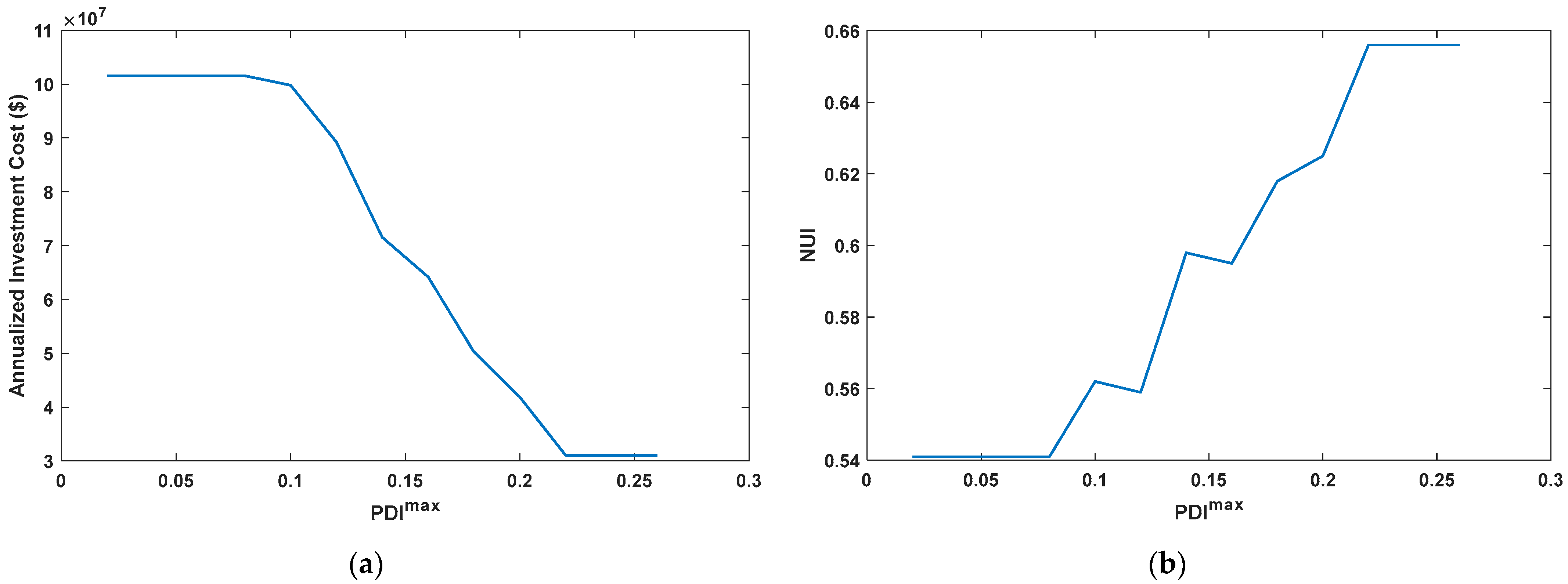
• Comparing case (a) with case (b) indicates that although PDI decreased from 0.208 to 0.090, the investment cost rose by 221%. However, the operation cost reduced by about 6.8% due to the more available capacity in the transmission grid, which yielded the commitment of cheaper generators. As expected, the objective function in case (b) would be 1.8% higher than in case (a). This increase was at the expense of reducing PDI. It is of note that NUI was slightly lower in case (b) when compared with case (a), indicating that transmission was less used in case (b).
• If NUI was considered to be the market power index in the TEP problem, it decreased to its minimum value of 0.399. However, both investment and operation cost increased in this case to lower the NUI. The objective function was 6.5% higher in case (c) compared with case (a). The PDI in case (c) was higher than that in case (b), but slightly lower than that in case (a).
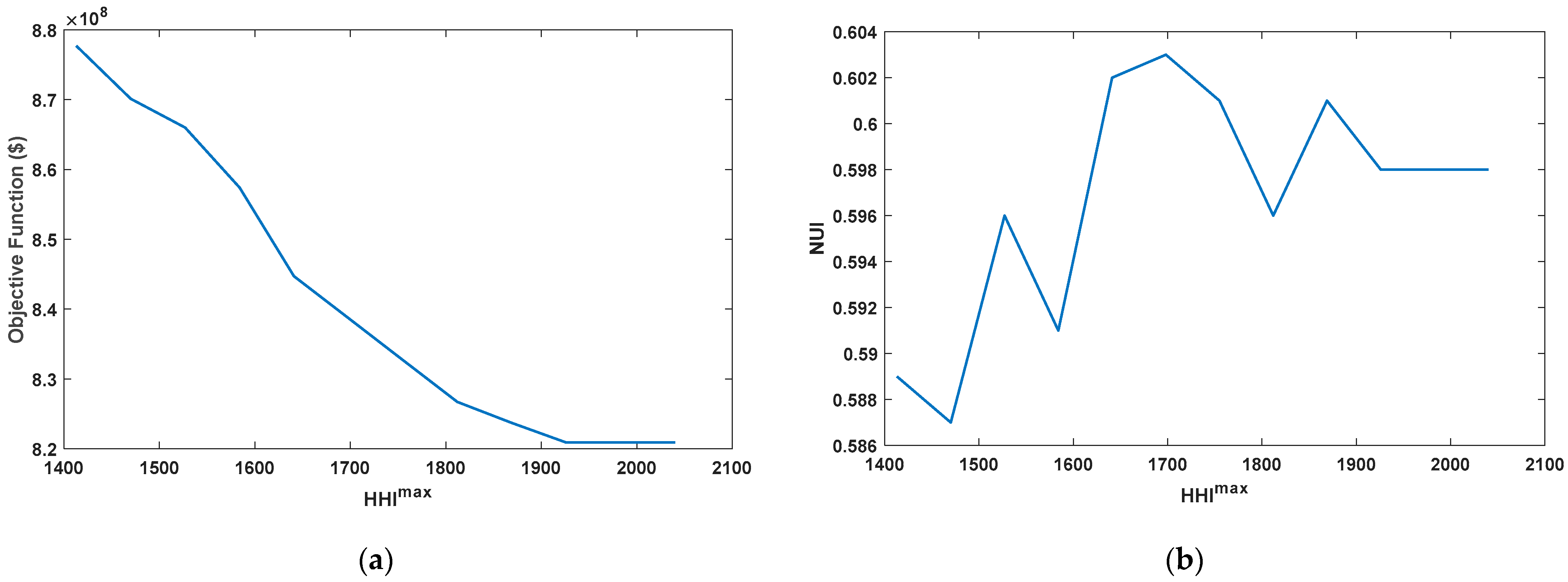
• In case (d), where HHI was considered as the market power index, the operation cost was the highest among all of the cases. To guarantee that constraint $HHI\le HH{I}_{}^{max}=100$ was satisfied, the more expensive generators were dispatched, leading to a greater total operation cost. As shown in Table 1, the operation cost was 9% higher than that in case (a). In addition, despite the higher investment cost in case (d) compared with case (a), NUI had the largest amount in case (d). HHI in the other three cases was above 100. Note that as the number of producers participating in the electricity generation was large enough (54 generators), all four cases were considered competitive electricity markets from the HHI point of view. The effect of the fewer generation companies on the HHI will be studied shortly.

It is of note that a linear combination of market power indices introduced in the previous section could also be used. For instance, let us consider $w\times PDI+\left(1-w\right)NUI\le MP{I}_{}^{max}=w\times PD{I}_{}^{max}+\left(1-w\right)NU{I}_{}^{max}$ as a combination of PDI and NUI. The results for different amounts of weighting factor $w$ are shown in

Table 2. Optimal solutions for four different cases considering different weighting factors.

	$\mathit{w}=0$ (Case (c))	$\mathit{w}=0.2$	$\mathit{w}=0.5$	$\mathit{w}=0.8$	$\mathit{w}=1$ (Case (b))
Annualized investment cost (×107$)	7.762	8.391	8.779	9.546	9.980
Operation cost (×108$/year)	7.967	7.812	7.604	7.479	7.358
Objective function (×108$)	8.743	8.651	8.481	8.433	8.356
PDI	0.189	0.153	0.117	0.097	0.090
NUI	0.399	0.423	0.487	0.509	0.541
HHI	175	171	170	166	163

. Notice that $w=0$ corresponded to case (c) and $w=1$ corresponded to case (b). It can be seen in Table 2 that as $w$ increased, the investment cost rose while the operation cost decreased. In addition, as expected, PDI reduced and NUI increased.

Figure 1 denotes the investment cost as well as NUI for case (b) for different values of $PD{I}_{}^{max}$. It was concluded from this figure that as $PD{I}_{}^{max}$ decreased, the investment cost of transmission lines increased, meaning that more transmission lines were needed to be built to mitigate the price deviation throughout the power system. For $PD{I}_{}^{max}$ equal to 0.21, (3) it was nonbinding, i.e., it could be removed without any changes in the optimal solution. Therefore, the investment cost remained unchanged for $PD{I}_{}^{max}\ge 0.21$. In addition, when $PD{I}_{}^{max}$ reached 0.08, the investment cost reached its maximum value of 10.157 × 10⁷$. For such an investment cost, PDI was zero, meaning there was no congestion in the expanded transmission grid in all of the scenarios. Moreover, it is observed from Figure 1 that, in general, as $PD{I}_{}^{max}$ increased, NUI increased as well, because more lines were constructed, which led to more available capacity in the network. However, when $PD{I}_{}^{max}$ increased from 0.10 to 0.12 or from 0.14 to 0.16, the NUI reduced a little despite the rise in transmission capacity. This could be justified because the power flow pattern through the transmission lines slightly changed as $PD{I}_{}^{max}$ increased.

To further analyze the results, Figure 2 plots the average locational marginal prices (LMPs) across the power system for three different values of $PD{I}_{}^{max}$. The blue curve shows the LMPs for $PD{I}_{}^{max}=0.21$. As can be seen, electricity prices differed significantly across the whole power system. For instance, the end-user at bus 78 would face a high electricity price of 37 USD/MWh, while the end-user at bus 12 would experience an electricity price as low as 3 USD/MWh. This means that access to open transmission capacity was not non-discriminatory. As $PD{I}_{}^{max}$ decreased from 0.21 to 0.16, the price volatility was reduced. For $PD{I}_{}^{max}$ equal to 0.10 (red curve), the price profile was much smoother than the other two curves, indicating that the presented mathematical model could effectively introduce more uniform prices across the network, but at the expense of building more transmission lines.

To investigate the effect of the number of players on HHI, we studied the simulation results for fewer generation companies. Notice that the number of players was assumed to be known before the planning process. In doing so, we assumed the number of generating companies to be 2, 5, and 10. The optimal solutions are shown in

Table 3. Optimal solutions considering different numbers of market players.

		Case (e): 2 Players	Case (f): 5 Players	Case (g): 10 Players
With HHI as MPI	HHI	3898	1413	649
	Annualized investment cost ($)	3.337 × 107	3.632 × 107	3.006 × 107
	Operation cost ($/year)	7.952 × 108	8.414 × 108	8.697 × 108
	Objective function ($)	8.289 × 108	8.777 × 108	8.997 × 108
Without MPI	HHI	4207	1926	893

. As expected, as the number of players grew, HHI reduced, regardless of whether HHI was included in the TEP problem or not. Furthermore, for all three cases, HHI decreased if it was considered in the TEP problem by 7.3%, 26%, and 27% for cases (e), (f), and (g), respectively. However, the cost to mitigate HHI was an increase in the objective function. It should be highlighted that when the number of players was 2, it was much more challenging to reduce HHI. Note that the investment and operation cost for the situation in which HHI was not considered in the TEP model was the same as case (a) and was not be impacted by the number of players because we did not model the competitive behavior of the market participant. In addition, the HHIs provided in row 2 of Table 3 were the minimum values of $HH{I}_{}^{max}$ under which the optimization model was feasible. This means if $HH{I}_{}^{max}$ was selected below the amounts given in Table 3, the problem was infeasible. Therefore, this is the minimum HHI that the planning model could achieve. Figure 3 illustrates the objective function and NUI for different values of $HH{I}_{}^{max}$, while the number of players was fixed at 5. As $HH{I}_{}^{max}$ increased from its minimum value, i.e., 1413, the objective function was reduced. When $HH{I}_{}^{max}$ reached 1926, the objective function did not change anymore. The right-hand side of Figure 3 indicates that NUI behaved randomly, and there was no correlation between $HH{I}_{}^{max}$ and the amount of NCI. It is of note that in a market with a higher competitiveness level, the total operation cost must be lower in practice, i.e., the higher the competition, the lower the operation cost. However, comparing cases (c) and (e) was inconsistent with this point. The reason is that the generation cost of each generator ($c_i^T$) was assumed to be a constant parameter for all cases. In fact, it was assumed that all generators submited their marginal cost. To consider the effect of different competition levels on the operation cost, we needed to model the bidding strategy in the problem, which was beyond the scope of our research work.

5. Conclusions

This paper presents a market-oriented TEP model that directly takes the market power measures into account. Motivated by the existing market settings, the proposed model incorporates the market power measures using an approximated lossless DC representation of power flow. In this context, a stochastic bilevel model is formulated where the planner makes investment decisions at the upper level while respecting the constraints associated with market power. The lower level is to clear the market using DC equations given the optimal decisions attained from the upper level. The solution strategy is based on the broadly used KKT conditions resulting in a MILP/MIQP problem whose solution algorithms are efficient and mature. A set of plausible scenarios represents wind power and electricity demand uncertainty. As demonstrated by the numerical experiment, the proposed model can effectively reduce the market power in the electricity market, but at the cost of a higher investment cost. The lower the market power indices, the higher the investment cost. Moreover, it is observed that the set of candidate transmission lines can significantly influence the results. It is also inferred from the numerical experiment that improving one of the market power indices for the same set of candidate lines does not necessarily lead to an improvement in all indices.

In future studies, we will model the generalizations of our formulation by investigating the possibility of incorporating AC power flow equations. In addition, as the generation expansion plans considerably affect the market power indices, it is suggested to consider the market power in a co-planning model for transmission and generation expansion. It is also interesting to explore the effect of demand response as well as energy storage systems on the market power in the planning problems.

References

1. Li, C.; Conejo, A.J.; Liu, P.; Omell, B.P.; Siirola, J.D.; Grossmann, I.E. Mixed-Integer Linear Programming Models and Algorithms for Generation and Transmission Expansion Planning of Power Systems. Eur. J. Oper. Res. 2022, 297, 1071–1082. [Google Scholar] [CrossRef]
2. Moreira, A.; Pozo, D.; Street, A.; Sauma, E.; Strbac, G. Climate-aware Generation and Transmission Expansion Planning: A Three-stage Robust Optimization Approach. Eur. J. Oper. Res. 2021, 295, 1099–1118. [Google Scholar] [CrossRef]
3. Kazemi, M.; Ansari, M.R. An Integrated Transmission Expansion Planning and Battery Storage Systems Placement-A Security and Reliability Perspective. Int. J. Electr. Power Energy Syst. 2022, 134, 107329. [Google Scholar] [CrossRef]
4. Bhattiprolu, P.A.; Conejo, A.J. Multi-Period AC/DC Transmission Expansion Planning Including Shunt Compensation. IEEE Trans. Power Syst. 2021, 37, 2164–2176. [Google Scholar] [CrossRef]
5. Mazaheri, H.; Moeini-Aghtaie, M.; Fotuhi-Firuzabad, M.; Dehghanian, P.; Khoshjahan, M. A Linearized Transmission Expansion Planning Model under N − 1 Criterion for Enhancing Grid-Scale System Flexibility via Compressed Air Energy Storage Integration. IET Gener. Transm. Distrib. 2022, 16, 208–218. [Google Scholar] [CrossRef]
6. Qorbani, M.; Amraee, T. Long Term Transmission Expansion Planning to Improve Power System Resilience against Cascading Outages. Electr. Power Syst. Res. 2021, 192, 106972. [Google Scholar] [CrossRef]
7. Mehrtash, M.; Cao, Y. A New Global Solver for Transmission Expansion Planning With AC Network Model. IEEE Trans. Power Syst. 2022, 37, 282–293. [Google Scholar] [CrossRef]
8. Liu, D.; Zhang, S.; Cheng, H.; Liu, L.; Zhang, J.; Zhang, X. Reducing Wind Power Curtailment by Risk-Based Transmission Expansion Planning. Int. J. Electr. Power Energy Syst. 2021, 124, 106349. [Google Scholar] [CrossRef]
9. Mortaz, E.; Valenzuela, J. Evaluating the Impact of Renewable Generation on Transmission Expansion Planning. Electr. Power Syst. Res. 2019, 169, 35–44. [Google Scholar] [CrossRef]
10. Gutiérrez-Alcaraz, G.; González-Cabrera, N.; Gil, E. An Efficient Method for Contingency-Constrained Transmission Expansion Planning. Electr. Power Syst. Res. 2020, 182, 106208. [Google Scholar] [CrossRef]
11. Vilaça Gomes, P.; Saraiva, J.T.; Carvalho, L.; Dias, B.; Oliveira, L.W. Impact of Decision-Making Models in Transmission Expansion Planning Considering Large Shares of Renewable Energy Sources. Electr. Power Syst. Res. 2019, 174, 105852. [Google Scholar] [CrossRef]
12. Zhuo, Z.; Du, E.; Zhang, N.; Kang, C.; Xia, Q.; Wang, Z. Incorporating Massive Scenarios in Transmission Expansion Planning With High Renewable Energy Penetration. IEEE Trans. Power Syst. 2020, 35, 1061–1074. [Google Scholar] [CrossRef]
13. Gomes, P.V.; Saraiva, J.T. A Two-Stage Strategy for Security-Constrained AC Dynamic Transmission Expansion Planning. Electr. Power Syst. Res. 2020, 180, 106167. [Google Scholar] [CrossRef]
14. Zhang, X.; Conejo, A.J. Candidate Line Selection for Transmission Expansion Planning Considering Long- and Short-Term Uncertainty. Int. J. Electr. Power Energy Syst. 2018, 100, 320–330. [Google Scholar] [CrossRef]
15. Wu, Z.; Liu, Y.; Gu, W.; Wang, Y.; Chen, C. Contingency-Constrained Robust Transmission Expansion Planning under Uncertainty. Int. J. Electr. Power Energy Syst. 2018, 101, 331–338. [Google Scholar] [CrossRef]
16. El-Meligy, M.; El-Sherbeeny, A.; Anvari-Moghaddam, A. Transmission Expansion Planning Considering Resistance Variations of Overhead Lines Using Minimum-Volume Covering Ellipsoid. IEEE Trans. Power Syst. 2021, 37, 1916–1926. [Google Scholar] [CrossRef]
17. El-Meligy, M.A.; Sharaf, M.; Soliman, A.T. A Coordinated Scheme for Transmission and Distribution Expansion Planning: A Tri-Level Approach. Electr. Power Syst. Res. 2021, 196, 107274. [Google Scholar] [CrossRef]
18. Zhan, J.; Liu, W.; Chung, C.Y. Stochastic Transmission Expansion Planning Considering Uncertain Dynamic Thermal Rating of Overhead Lines. IEEE Trans. Power Syst. 2019, 34, 432–443. [Google Scholar] [CrossRef]
19. Liang, Z.; Chen, H.; Chen, S.; Lin, Z.; Kang, C. Probability-Driven Transmission Expansion Planning with High-Penetration Renewable Power Generation: A Case Study in Northwestern China. Appl. Energy 2019, 255, 113610. [Google Scholar] [CrossRef]
20. Sun, M.; Cremer, J.; Strbac, G. A Novel Data-Driven Scenario Generation Framework for Transmission Expansion Planning with High Renewable Energy Penetration. Appl. Energy 2018, 228, 546–555. [Google Scholar] [CrossRef] [Green Version]
21. Gbadamosi, S.L.; Nwulu, N.I. A Multi-Period Composite Generation and Transmission Expansion Planning Model Incorporating Renewable Energy Sources and Demand Response. Sustain. Energy Technol. Assess. 2020, 39, 100726. [Google Scholar] [CrossRef]
22. Nemati, H.; Latify, M.A.; Yousefi, G.R. Coordinated Generation and Transmission Expansion Planning for a Power System under Physical Deliberate Attacks. Int. J. Electr. Power Energy Syst. 2018, 96, 208–221. [Google Scholar] [CrossRef]
23. Zahedi Rad, V.; Torabi, S.A.; Shakouri, G.H. Joint Electricity Generation and Transmission Expansion Planning under Integrated Gas and Power System. Energy 2019, 167, 523–537. [Google Scholar] [CrossRef]
24. Wang, J.; Zhong, H.; Tang, W.; Rajagopal, R.; Xia, Q.; Kang, C. Tri-Level Expansion Planning for Transmission Networks and Distributed Energy Resources Considering Transmission Cost Allocation. IEEE Trans. Sustain. Energy 2018, 9, 1844–1856. [Google Scholar] [CrossRef]
25. Roldán, C.; Sánchez de la Nieta, A.A.; García-Bertrand, R.; Mínguez, R. Robust Dynamic Transmission and Renewable Generation Expansion Planning: Walking towards Sustainable Systems. Int. J. Electr. Power Energy Syst. 2018, 96, 52–63. [Google Scholar] [CrossRef] [Green Version]
26. Gomes, P.V.; Saraiva, J.T. State-of-the-Art of Transmission Expansion Planning: A Survey from Restructuring to Renewable and Distributed Electricity Markets. Int. J. Electr. Power Energy Syst. 2019, 111, 411–424. [Google Scholar] [CrossRef]
27. Naderi, E.; Pourakbari-Kasmaei, M.; Lehtonen, M. Transmission Expansion Planning Integrated with Wind Farms: A Review, Comparative Study, and a Novel Profound Search Approach. Int. J. Electr. Power Energy Syst. 2020, 115, 105460. [Google Scholar] [CrossRef]
28. Mahdavi, M.; Antunez, C.S.; Ajalli, M.; Romero, R. Transmission Expansion Planning: Literature Review and Classification. IEEE Syst. J. 2019, 13, 3129–3140. [Google Scholar] [CrossRef]
29. Hemmati, R.; Hooshmand, R.-A.; Khodabakhshian, A. State-of-the-Art of Transmission Expansion Planning: Comprehensive Review. Renew. Sustain. Energy Rev. 2013, 23, 312–319. [Google Scholar] [CrossRef]
30. Ude, N.G.; Yskandar, H.; Graham, R.C. A Comprehensive State-of-the-Art Survey on the Transmission Network Expansion Planning Optimization Algorithms. IEEE Access 2019, 7, 123158–123181. [Google Scholar] [CrossRef]
31. Cardell, J.B.; Hitt, C.C.; Hogan, W.W. Market Power and Strategic Interaction in Electricity Networks. Resour. Energy Econ. 1997, 19, 109–137. [Google Scholar] [CrossRef]
32. Borenstein, S.; Bushnell, J.; Kahn, E.; Stoft, S. Market Power in California Electricity Markets. Util. Policy 1995, 5, 219–236. [Google Scholar] [CrossRef]
33. Harvey, S.M.; Hogan, W.W. Hogan Nodal and Zonal Congestion Management and the Exercise of Market Power; Harvard University: Cambridge, MA, USA, 2000. [Google Scholar]
34. Joskow, P.; Schmalensee, R.L. Market for Power: An Analysis of Electric Utility Deregulation; MIT Press: Cambridge, MA, USA, 1983. [Google Scholar]
35. Awad, M.; Broad, S.; Casey, K.E.; Chen, J.; Geevarghese, A.S.; Miller, J.C.; Perez, A.J.; Sheffrin, A.Y.; Zhang, M.; Toolson, E.; et al. The California ISO Transmission Economic Assessment Methodology (TEAM): Principles and Application to Path 26. In Proceedings of the 2006 IEEE Power Engineering Society General Meeting, Montreal, QC, Canada, 18–22 June 2006; p. 8. [Google Scholar]
36. Aguado, J.A.; De La Torre, S.; Contreras, J.; Conejo, A.J.; Martínez, A. Market-Driven Dynamic Transmission Expansion Planning. Electr. Power Syst. Res. 2012, 82, 88–94. [Google Scholar] [CrossRef]
37. Wang, P.; Xiao, Y.; Ding, Y. Nodal Market Power Assessment in Electricity Markets. IEEE Trans. Power Syst. 2004, 19, 1373–1379. [Google Scholar] [CrossRef]
38. Shang, N.; Ding, Y.; Cui, W. Review of Market Power Assessment and Mitigation in Reshaping of Power Systems. J. Mod. Power Syst. Clean Energy 2021, 10, 1067–1084. [Google Scholar] [CrossRef]
39. Gurobi Optimization. Gurobi Optimizer Reference Manual. Available online: http://Www.Gurobi.Com (accessed on 1 March 2022).
40. Guide, G.U. GAMS Development Corporation: Washington, DC, USA. Available online: https://Www.gams.Com (accessed on 1 March 2022).
41. Data for “A Bilevel Stochastic Optimization Framework for Market-Oriented Transmission Expansion Planning Considering Market Power”. Available online: https://Drive.Google.Com/File/d/1iESlgO9YTV2DBZGMYFicSAkTuJvDQ7X2/View?Usp=sharing (accessed on 1 March 2022).
Figure 1. (a) Annualized investment cost of transmission lines and (b) NUI versus different values of P D I m a x .
Energies 16 03256 g001
Figure 2. Average LMPs at different buses versus different values of P D I m a x .
Energies 16 03256 g002
Figure 3. (a) Objective function and (b) NUI versus different values of H H I m a x for the number of players being 5.
Energies 16 03256 g003