Article

A Hybrid Approach of the Deep Learning Method and Rule-Based Method for Fault Diagnosis of Sucker Rod Pumping Wells

School of Petroleum and Natural Gas Engineering, Changzhou University, Changzhou 213164, China
*
Author to whom correspondence should be addressed.
Energies 2023, 16(7), 3170; https://doi.org/10.3390/en16073170
Submission received: 3 March 2023 / Revised: 24 March 2023 / Accepted: 28 March 2023 / Published: 31 March 2023
(This article belongs to the Section H1: Petroleum Engineering)

Abstract

:
Accurately obtaining the working status of the sucker rod pumping wells is a challenging problem for oil production. Sensors at the polished rod collect working data to form surface dynamometer cards for fault diagnosis. A prevalent method for recognizing these cards is the convolutional neural network (CNN). However, this approach has two problems: an unbalanced dataset due to varying fault frequencies and similar dynamometer card shapes that complicate recognition. This leads to a low accuracy of fault diagnosis in practice, which is unsatisfactory. Therefore, this paper proposes a hybrid approach of the deep learning method and rule-based method for fault diagnosis of sucker rod pumping wells. Specifically, when the CNN model alone fails to achieve satisfactory accuracy in the working status, historical monitoring data of the relevant wells can be collected, and expert rules can assist CNN to improve diagnostic accuracy. By analyzing time series data of factors such as the maximum and minimum loads, the area of the dynamometer card, and the load difference, a knowledgebase of expert rules can be created. When performing fault diagnosis, both the dynamometer cards and related time series data are used as inputs. The dynamometer cards are used for the CNN model to diagnose, and the related time series data are used for expert rules to diagnose. The diagnostic results and the confidence levels of the two methods are obtained and compared. When the two diagnostic results conflict, the one with higher confidence is preserved. Out of the 2066 wells and 7 fault statuses analyzed in field applications, the hybrid approach demonstrated a 21.25% increase in fault diagnosis accuracy compared with using only the CNN model. Additionally, the overall accuracy rate of the hybrid approach exceeded 95%, indicating its high effectiveness in diagnosing faults in sucker rod pumping wells.

1. Introduction

The sucker rod pumping system is still the primary artificial lifting method in the oil industry to this day. The working environment of oil wells is complex and harsh. When faults occur during long-term operation, such as scaling problems and paraffin deposition, it not only causes a loss of crude oil production but may even lead to stringent safety and environmental accidents [1,2]. Therefore, promptly and accurately monitoring the working status of sucker rod pumping wells is vital for the safe production and improved recovery of oil fields.
After decades of research and exploration, analyzing the curve of a dynamometer card has become a common approach for diagnosing faults in sucker rod pumping wells [3]. This approach typically involves two processes: feature extraction and pattern recognition. During the feature extraction process, the two-dimensional data of the dynamometer card are transformed into one-dimensional features, such as eight-direction chain codes and spectrum analysis [4,5]. However, this transformation results in a loss of a large amount of useful information, making it difficult to distinguish specific faults and statuses [6]. One approach to the pattern classification process is to compare the differences between actual and known features of dynamometer cards, such as expert system and support vector machines [7,8]. Still, the complexity of oil reservoir and wells make it difficult to obtain dynamometer card templates for all oil reservoirs and working statuses [9]. Another approach is to build classification models on the basis of training data sets, such as different artificial neural network (ANN) structures [10,11]. Convolutional neural networks (CNN) learn the spatial structure of images adaptively through convolution and pooling, making neural networks much more powerful for image processing [12]. Studies by many scholars prove that fault diagnosis of sucker rod pumping wells has achieved great success after the application of CNN. The CNN model was used to predict the paraffin deposit with dynamometer cards. The accuracy rate of prediction was 98.08% [13]. A CNN model was designed for fault diagnosis, which could diagnose 30 types of fault statuses, and the training accuracy for all working status was greater than 95% [14].
Although the methods based on deep learning currently show great potential, the method requires a large sample base for training, and a series of problems still exist to be solved [15,16]. The frequency of occurrence of different working statuses is not the same during oil well production. Some working statuses, such as insufficient fluid supply and gas influence, occur every day in many wells and can accumulate a large number of data samples. However, some working statuses, such as sudden sucker rod break and valve leakage, occur less frequently and may not happen once a year for an oil well. These faults are far more hazardous than common statuses and require more attention. For the deep learning method, the data sample size of common working statuses is significant, while that of rare working statuses is still very insufficient [14]. As a result, the identification accuracy of rare working status is still not ideal in the training process. In addition, due to the complexity of the wells, many working status have a similar shape to the dynamometer card, such as sudden sucker rod break and pumping with gushing. Therefore, relying solely on the dynamometer card for diagnosis is prone to confusion [3]. Some statuses, such as paraffin deposition, is a slow-developing processes that cannot be judged only by the data of a single point in time; thus, they need to be considered comprehensively by the development trend of the past period [13]. The accuracy of the current method based solely on CNN is still insufficient due to the above problems.
To solve the problem caused by dynamometer card samples, some scholars used self-coding networks to increase the number of sample sets, as the generated dynamometer cards of partial fault status are missing essential features [17]. A real-time diagnosis method used a variety of wellbore parameters to assist in the fault diagnosis of CNN. At the same time, there are still difficulties in the collection of each parameter of the wellbore [18]. The above-mentioned studies have conducted some explorations of using neural network methods to improve accuracy, but the problem of applicability is still not well solved. With the continuous development of deep learning theory, coupling expert rules with deep learning method has attracted more attention as a new path to solving the above problems [19,20]. This combination has been applied in many similar scenarios with the fault diagnosis of sucker rod pumping wells, such as autonomous driving and medical diagnosis [21,22]. These scenarios all require solving the problem of image multi-classification. In medical diagnosis, doctors used expert rules to assist CNN with the classification of electrocardiograms, which can effectively solve the problem of misdiagnosis caused by similar electrocardiograms [22]. The application in these areas proves the feasibility of combining CNN and rules.
This study integrates the advantages of deep learning and rule-based method to construct a fault diagnosis method for sucker rod pumping wells. The CNN model and knowledgebase of expert rules are built by analyzing the data of sucker rod pumping wells over the years. The superiority of hybrid approach is verified by comparing the CNN model and the coupled approach. The hybrid approach is applied to oil production, relying on the experience of experts and the analysis of historical data. The diagnosis results of expert rules can compensate for the problems of CNN, and the results prove that it can improve the accuracy and interpretability of fault diagnosis.
The organization of this paper is as follows. Section 2 discusses the data collected and used in this paper. Section 3 describes the reason of low accuracy working statuses and the method to build knowledgebase of fault diagnosis. Section 4 represents the architecture of the CNN model. Section 5 shows the combination of CNN with the rule-based method, and the effectiveness of the hybrid approach is verified after being applied in an oil field. Finally, Section 6 presents the research conclusions.

2. Data Gathering and Preprocessing

With the implementation of digital oil fields, various sensors installed on the sucker rod pumping system can continuously transmit data to the data center, treating the sucker rod of a rod pump as a transmission conductor, using load sensors and displacement sensors to receive the instantaneous load and displacement signals on the ground polished rod, digitizing the signals generated by the two sensors, and submitting some well data (sucker rod length, weight, cross-sectional area, etc.) to microcomputer operation processing to obtain instantaneous load and displacement data of the sucker rod.
For example, consider the X oil field, which has 300 wells and collects data every half an hour. To diagnose the current working status of a well, data collected from the current moment up to the past 7 days will be gathered to form a data sample. The sample includes displacement and load data during the current stroke cycle, as well as the maximum load, minimum load, and area of the dynamometer card over the past 7 days. These data can be directly obtained from the database. Additionally, the load difference is calculated on the basis of the maximum load and minimum load and included in the sample. Displacement and load are vectors, each consisting of 200 data points representing the displacement and load corresponding to a time point in one stroke cycle. A current dynamometer card can be generated using the displacement and load vectors. The maximum load, minimum load, area of the dynamometer card, and load difference are time series consisting of 336 data points each, representing data recorded every half an hour over the past 7 days. The details are presented in Table 1.
In this paper, an analysis of characteristic parameters from various working statuses revealed that the maximum load, minimum load, area of the dynamometer card, and load difference form four vectors that consist of time series data. The final point in each vector represents the current well status, reflecting the working status of the sucker rod pumping system to a certain extent over the past seven days. Hence, expert rules were established around the variation range of these four parameters to create a knowledgebase for each fault status. These expert rules can effectively assist in logical reasoning for diagnosing the fault statuses.
Drawing a dynamometer card is a prerequisite for preparing a sample set for deep learning. The original data of the dynamometer card is stored in the database in the form of displacement vectors (W) and load vectors (Z). The displacement vector and load vector record the suspended displacement and load of 200 sampling points during the up and down stroke process of the pumping well. By using displacement and load as the x and y coordinates, the curve of the relationship between displacement and load obtained by plotting in a Cartesian coordinate system is called the dynamometer card. To ensure that the dynamometer card can show its characteristics, the normalized processing ordinate axis takes a range of values as [max(minZ,0), maxZ], and the abscissa axis takes a range of values as [minW, maxW], The image size is 64 × 48 pixels. The dynamometer card shown contains axes, but they are removed when used as a training set for deep learning. All dynamometer cards used in this paper are drawn to this standard. The samples displayed and trained are derived from data corresponding to the pump inspection results, ensuring that the dynamometer card conforms to the marked working status.
Figure 1, Figure 2, Figure 3, Figure 4, Figure 5, Figure 6 and Figure 7 show the dynamometer cards of various working statuses.

3. Rule-Based Method for Fault Diagnosis

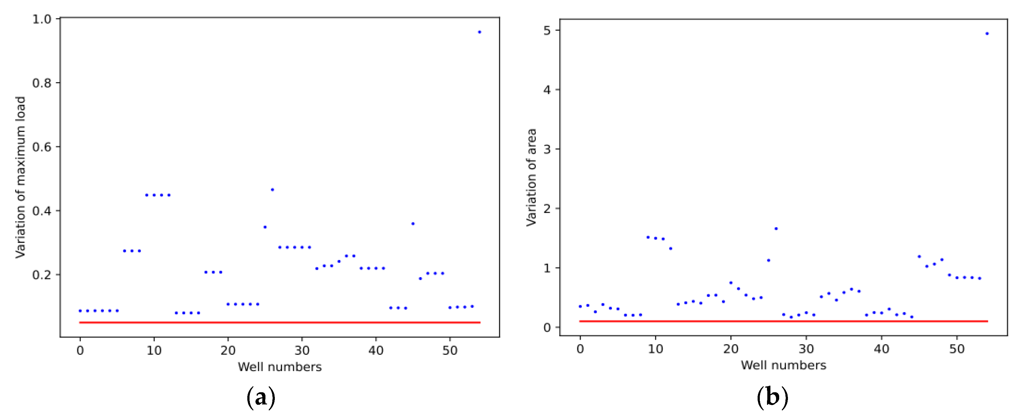
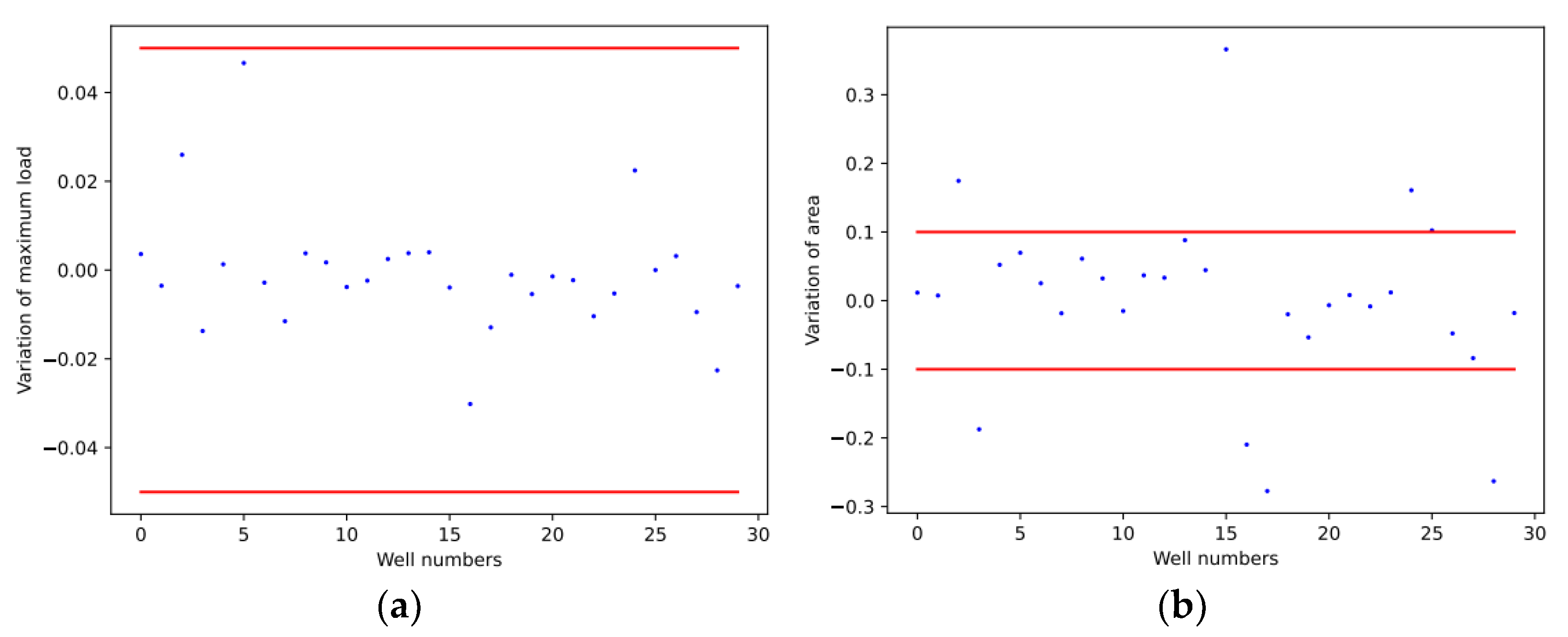
3.1. Analysis of Low Accuracy Working Status

The core unit of a sucker rod pumping well is the pump, located in the lower part of the pumping unit’s polished rod and submerged in the fluid at the bottom of the well during operation. The pumping team works with the help of a piston driven by a traveling valve, a standing valve, a plunger, and a pump barrel to collect crude oil. The traveling valve, which follows the plunger in its cyclic motion, is located on the plunger in the pump barrel and helps to remove the crude oil from the barrel. In contrast, the standing valve in the lower part of the barrel opens upwards to draw the crude oil into the barrel. During the pumping process, the standing valve position remains unchanged, and the plunger moves up and down in one cycle called one stroke.
The surface dynamometer card is a closed curve of displacement and load in one stroke. The value of displacement and load changes of the rod under different working statuses for various reasons will eventually be reflected in the shape of the curve. Therefore, the shape of the dynamometer card can reflect the working status of the sucker rod pumping system to a certain extent [23]. The following is an analysis of several fault situations and their corresponding surface dynamometer cards. The dynamometer card mentioned in this paper is regarded as the surface dynamometer card if not specifically stated. Due to the limited data available, the dynamometer cards used and presented in this paper represent only the wells for which data were collected; thus, they may have unique characteristics and cannot be used as typical dynamometer cards.
At present, the diagnostic accuracy is still insufficient under these statuses:
(1)
Low-frequency status
Oil well valve leakage is a relatively rare occurrence; it does not happen several times a year in a single well. For example, in an oil reservoir over the past year, 39,488 samples with insufficient liquid supply were collected, and only 140 valve leakage samples were collected. If we use this sample set to train a machine learning model without any data balancing measures, the model will learn about insufficient liquid supply 282 times more than valve leakage, resulting in inaccurate diagnosis of valve leakage.
Figure 8a shows the dynamometer card of traveling valve leakage. The pressure inside the pump decreases during the upstroke, which creates a pressure difference between the two ends of the plunger, and the liquid leaks to the pump barrel under the plunger through the discharge part of the unconsolidated pump, for example, the opening between the traveling valve and the plunger. The leakage rate increases due to the decrease in the pressure under the plunger. Leakage leads to the suspension point load not reaching the maximum value, resulting in the maximum load decline, and decreasing the area of the dynamometer card.
Figure 8b shows the dynamometer card of standing valve leakage. It is not possible to increase the pressure of the pump promptly during the downstroke, which slows down the unloading process, and so the traveling valve cannot be opened immediately. When the plunger speed is faster than the leakage speed, it increases to a higher pressure than the liquid column pressure in the pump, but the plunger speed decreases, and the pressure in the pump causes the standing valve to close early, making the suspension point unload early. This results in a decrease in the maximum load and a decrease in the area of the dynamometer card.
(2)
Status of the dynamometer cards have similar shapes
As shown in Figure 9, it is evident that the two dynamometer cards of sudden sucker rod break and pumping with gushing are very similar, as both appear to be as narrow, thin lines with a small distance between the upstroke and downstroke. When the sucker rod breaks suddenly, the polished rod load becomes equal to the weight of the sucker rod above the break point. However, the top and bottom lines of load do not match because of the friction in the wellbore. The sudden break causes a sharp drop in load.
(3)
Gradually changing status
Paraffin deposition is gradual, and the surface dynamometer card does not change suddenly and drastically. Due to the paraffin deposition, the piston resistance increases throughout the stroke or in a certain area. The additional resistance on the upstroke increases the polished rod load; the additional resistance on the downstroke decreases the polished rod load. This causes the maximum load to increase and the minimum load to decrease. As shown in Figure 10, the paraffin deposition becomes more severe, and the dynamometer card gradually becomes more expansive. This status cannot be judged by the dynamometer card at a single point in time, and in the early phase, the dynamometer card has no noticeable change compared with the normal status.
The shape of the surface dynamometer card in actual oilfield sites may differ from the theoretical dynamometer card of various fault statuses due to factors such as geology and reservoir type. This may cause some fault statuses to look similar on the dynamometer card. Some fault statuses gradually changing cannot be judged by one dynamometer card alone. Therefore, using only CNN to analyze the dynamometer card may reduce the diagnostic accuracy of these fault statuses.

3.2. Fault Diagnosis Knowledgebase

In this study, by analyzing the historical production data of actual sucker rod pumping systems and combining the working experience of oilfield experts, the characteristic parameters of fault statuses are extracted and summarized to provide data support for the construction of fault diagnosis knowledgebase. Given the limited number of wells available for the study, it was not possible to summarize expert rules for a large number of another working statuses. Nevertheless, several typical fault statuses were selected to verify the feasibility of the method.
The collected data format is shown in Section 2, each time series is X = x 1 , x 2 , x n , and the formula for calculating the variation in the time series is as Equation (1).
λ = x n o w x m e a n x m e a n
where λ indicates the variation, xnow is xn, which is the current value, and xmean is the mean value of the series.
Fault diagnosis requires timeliness, and current data are more meaningful than data from the past. The average value represents the overall situation of the past period to avoid the interference of sudden maximum or minimum values. To ensure consistency of the results, the average value is subtracted from the current value, then the resulting difference is divided by the average value. This generates a ratio that represents the variation, which is more convenient for comparison and use. The calculation results are not taken as absolute values, whereas the positive or negative results of the magnitude of change calculation represent the rise or fall of the characteristic parameters. Figure 11, Figure 12, Figure 13, Figure 14 and Figure 15 show the variation in characteristic parameters corresponding to various working statuses.
By analyzing the time series of various fault statuses through Equation (1), the regularity of the fault status and its corresponding maximum load, minimum load, surface dynamometer card area, and load difference changes are obtained, and a knowledgebase of the expert rules is built on the basis of this. Consider paraffin deposition as an example; the data of all wells were processed by Equation (1), and it found that their area of dynamometer card and maximum load had certain regularity. As shown in Figure 11, Figure 12, Figure 13, Figure 14 and Figure 15, the blue dots indicate the magnitude of change of the corresponding characteristic parameters for each well, and the upper half-axis of Y indicates that the trend of the characteristic parameters is rising. The red line indicates the threshold value of the variation magnitude, and the blue dots are all above the red line, which indicates that the data of all wells meet the set threshold value. Therefore, the fault status can be deduced as paraffin deposition on the basis of the maximum load rise >5% and the area of surface dynamometer card rise > 10%. Other fault statuses are also analyzed this way, and the laws are summarized into a knowledgebase.
Table 2 shows the statistical fault statuses and their characteristic parameter variations.
The knowledge expressed by the method in the knowledgebase constructed in this paper is a production rule, which is described by the following means:
Rule No.: IF condition, THEN action
Production rules have the form of IF condition THEN action, where the condition is the condition of this rule, and action is the conclusion of this rule. Production rules can describe the relationship between conditions and conclusions in facts concisely and clearly, the conditions and conclusions can be combined by logical operations, weighting factors can be added to the rules to make them gain weighted uncertainty, and many rules can be connected to form a rule base. The causal conditions of the production rules must all be satisfied to be valid, otherwise the conclusion cannot be deduced if one of the conditions is satisfied singly.
Based on the characteristics of the fault status parameters, the following knowledgebase of the expert rule is summarized.
R1: IF Maximum load drop >2.5% and Area of surface dynamometer card drop >10%, THEN Traveling valve leakage (Confidence: 0.5);
R2: IF Maximum load drop >2.5% and Area of surface dynamometer card drop >10%, THEN Standing valve leakage (Confidence: 0.5);
R3: IF Maximum load drop >10% and Load difference drop >45%, THEN Sudden sucker rod break (Confidence: 0.8);
R4: IF Maximum load rise >5% and Area of surface dynamometer card rise >10%, THEN Paraffin deposition (Confidence: 0.7);
R5: IF Maximum load variation is within ±5% and Area of surface dynamometer card is within ±10%, THEN Pumping with gushing (Confidence: 0.9).
Despite the expert experience and data support, the accuracy of fault diagnosis using expert rules alone is still low because there are statuses with the same production rules, such as traveling valve leakage and standing valve leakage, which leads to lower confidence in the expert rules for both statuses. However, such statuses are distinguishable by the dynamometer card’s shape; thus, CNN is also needed to combine expert rules for fault diagnosis.

4. Deep Learning Method for Fault Diagnosis

Since the processing object is the dynamometer card, the selected neural network model is the convolutional neural network (CNN), which has powerful image processing capability. CNN is a popular algorithm in computer vision, having been successfully applied in domains such as autonomous driving and medical image processing. CNN is inspired by the cognitive mechanism of animal vision and simulates how visual cortex cells receive and analyze optical signals. CNN extracts and processes spatial hierarchical information of images through layers of visual neurons. A CNN consists of three types of layers: convolutional, pooling, and fully connected. The convolutional layer uses different sizes of convolutional kernels to extract various features from the input image. The pooling layer reduces the feature dimensionality by under-sampling. The fully connected layer maps the extracted features to the output result using a classifier.
LeNet-5 is a network model proposed by Y. Lecun in 1998 for handwritten digit recognition. It consists of three fully connected layers, two convolutional layers, and two pooling layers [24]. AlexNet is an improved network architecture based on LeNet-5, proposed by A. Krizhevsky in 2012. It has three convolutional layers followed by pooling layers, and three consecutive convolutional layers before accessing three fully connected layers [25]. To enhance the recognition and classification accuracy, AlexNet uses the ReLU activation function instead of the Tanh activation function in the convolutional layers. It also uses maximum pooling instead of average pooling to avoid blurring the image features. The dropout layer is added in the fully connected layer to proportionally eliminate some corresponding parameters and prevent overfitting.
This paper proposes a convolutional neural network architecture based on AlexNet and LeNet-5 models and consists of two convolutional layers, two pooling layers, and two fully connected layers. The convolutional layers use 3 × 3 convolutional kernels, and the pooling layers use 3 × 3 maximum pooling. The input image size is 64 × 48. Table 3 and Figure 16 show the structure of the network.
The network uses ReLU as the activation function between each layer except the output layer and Softmax as the activation function of the output layer to output the confidence level of the fault diagnosis category.
The ReLU and Sotfmax equations are as follows:
s o f t m a x i ( x ) = e x i j = 1 J e x j , i = 1 , 2 , 3 , , J
r e l u i ( x ) = max ( 0.2 , e x i ) , i = 1 , 2 , 3 , , J
where x indicates the vector of neuron parameters in the neural network; xi and xj indicate the ith and jth neuron parameters, respectively; i and j indicate the neuron number; and J indicates the total number of neurons in the neural network layer.
The neural network has three dropout layers to reduce the training time and prevent overfitting. Dropout layers randomly deactivate some neurons to lower the computational cost of the network model and enhance its generalization ability.

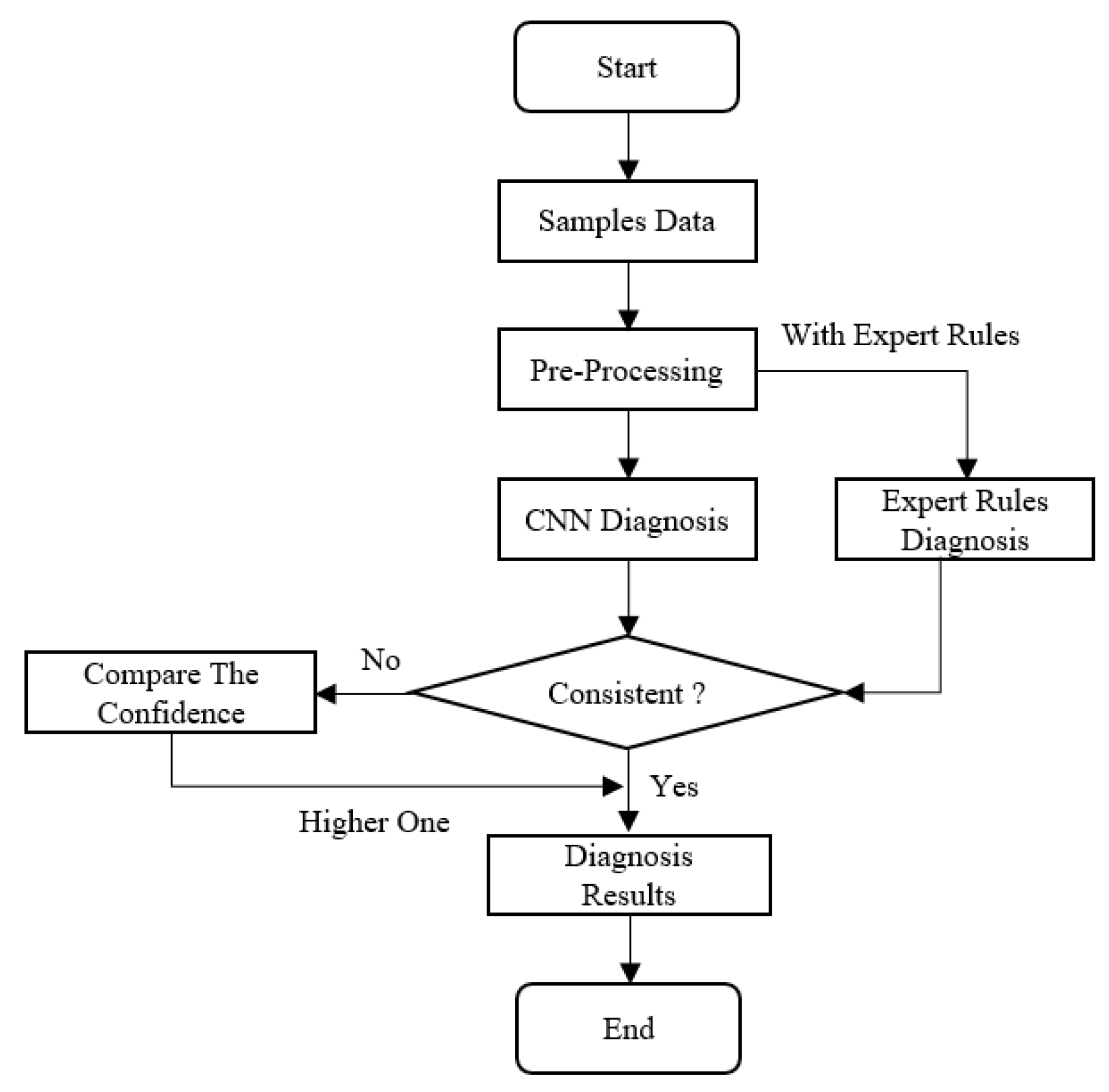
5. Combination of CNN and Expert Rules

Deep learning can build a neural network to fit the prediction function and learn the key features hidden in the massive data to infer and analyze the fault type. The inference and recognition process of rules is more rigorous than a neural network, and the rules are based on the technical and subjective experience accumulated in human history, which is hard to learn from the data set alone. The combination of CNN and expert rules can use expert rules to refine and complement the output of CNN and achieve mutual correction of both fault diagnosis results. Figure 17 shows the flowchart for fault diagnosis of this combined model.
The neural network outputs a vector of length 7, such as V p r e d i c t i o n = [ ( v p r e d i c t i o n ) 1 , , ( v p r e d i c t i o n ) j , ( v p r e d i c t i o n ) 7 ] , which represents the confidence levels for the seven fault statuses. Since the output layer uses Softmax as the activation function, the sum of the seven confidence levels is 100%, and the one with the highest confidence level is usually taken as the neural network’s diagnostic opinion. When the sample set is imbalanced or the dynamometer card of a fault type has a similar outline to other faults, the neural network’s confidence level will decrease and may be lower than the expert rule’s confidence level. In this case, mutual correction can improve the accuracy of fault diagnosis.
For fault diagnosis, both dynamometer cards and related time series data are used as inputs. The dynamometer cards are input to the CNN model for diagnosis, and the related time series data are input to the expert rules for diagnosis. The diagnostic results and confidence levels of both methods are obtained and compared. When there is a conflict between them, the one with higher confidence is retained.

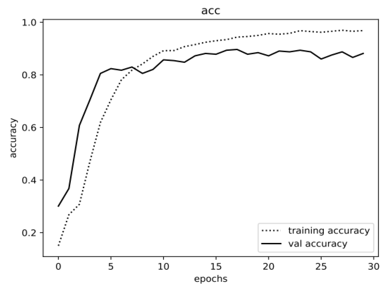
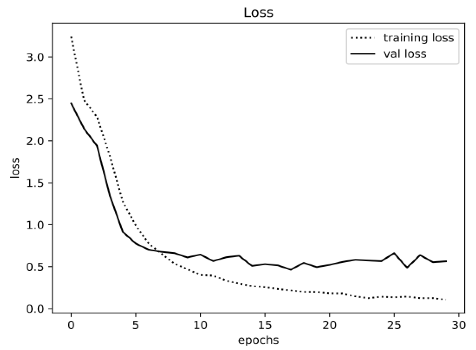
5.1. Training and Testing

CNN training is the process of finding the optimal weights for the neurons in each layer and storing them in a way that mimics the human brain’s memory. The training data are input to the model and the forward propagation and loss function calculate the difference between the current model prediction and the true value. Then, backward propagation and optimizer update the neuron weights in the neural network. This process is repeated until the model converges.
This study uses the cross-entropy loss function to train the convolutional neural network model. It is a loss function for multi-classification tasks that can measure the distance between two probabilities.
The expression is as follows.
C = 1 n k = 1 n y k ln a k + 1 y k ln 1 a k
where n is the total number of samples; k is the sample number; ak is the output value of the kth sample; y is the label value; and yk is the label value of the kth sample.
For the training process, we randomly split the sample set into 80% for training and 20% for validation. We trained the model for 30 epochs using Keras and Tensorflow (Keras and Tensorflow are open-source machine learning platforms, developed and maintained by Google Brain, in Mountain View, CA, USA). The running configuration was: Win10 64 bit; Intel i3-12100F 3.30 Ghz; AMD 6500xt; 16G Memory.
Figure 18 and Figure 19 show the training accuracy and loss values. After 20 epochs, the accuracy and loss values reached a plateau. The training accuracy and loss images indicate a gap between the training accuracy and the validation accuracy, which is consistent with the characteristics of using imbalanced samples to train the neural network [26].

5.2. Result of Fault Diagnosis

The test data used in the experiment were obtained from an oilfield site as mentioned in Section 2. Table 4, Table 5, Table 6, Table 7 and Table 8 show the detailed input and output parameters of the hybrid model. Since the vector of insufficient liquid supply and normal status have no obvious characteristics, the dynamometer card samples are sufficient, and CNN alone can effectively identify them. Therefore, these two working statuses are not discussed and only serve as a comparison.
Considering paraffin deposition as an example, fault diagnosis involves plotting the displacement and load vectors as a dynamometer card, similar to Figure 1 but without the axes, and inputting it into the CNN model. The CNN processing result is based on Equation (2), which outputs a vector of length equal to the number of classifications. In this paper, there are 7 categories: (normal, insufficient liquid supply, traveling valve leakage, standing valve leakage, sudden sucker rod break, paraffin deposition, and pumping with gushing). The points in this vector represent the confidence of each fault status, and their sum is 1. For this fault status, the maximum value in the vector is 0.3180 for the second item, which corresponds to the result of the CNN diagnosis indicating insufficient fluid supply (Confidence: 0.32). However, this prediction result has very low confidence, proving that this status is easily confused with other statuses when judged solely by the CNN model. To overcome this limitation, the related vector is processed using Equation (1) to calculate the variation of each characteristic parameter and compare this variation with the knowledgebase established in Section 3.2. If the variation conforms to the rules defined in R4, the output of the expert rule is paraffin deposition (Confidence: 0.7). The confidence of the expert rule is greater than that of the CNN model, which indicates that the output result is more reliable. If both confidence of outputs are not high, the higher is still used as the diagnosis. This approach is also applied to diagnose other fault statuses in the field.
Table 9 shows the accuracy rates of fault diagnosis using the CNN model and the hybrid approach on the sample set. The accuracy is calculated as the ratio of correctly diagnosed samples to all samples. The oil field had limited sample availability, so the training sets for normal and insufficient liquid supply were larger than the other five fault categories. The neural network alone performed well in diagnosing normal and insufficient fluid supply because they had sufficient training sets and clear dynamometer card features. However, the neural network alone had lower diagnostic accuracy for the other five fault categories due to insufficient training data or similarity to other faults on the dynamometer card. The hybrid approach improved the accuracy of diagnosing these faults by adding expert rules. For faults that had obvious rule features, such as sudden sucker rod break, paraffin deposition, and pumping with gushing, the diagnosis accuracy increased significantly after combining expert rules and even reached 100% in the field application test. Since normal and insufficient liquid supply had no obvious feature rule to diagnose them and had sufficient data available in the field, we did not test them with the coupling model.

6. Conclusions

For the problem of fault diagnosis of sucker rod pumping wells, the biggest problem is still the lack of available data. The main contribution of this paper is to create a hybrid of the CNN and expert rules for diagnosing sucker rod pump wells. The use of the oilfield field proves that this knowledgebase can compensate for the low accuracy of CNN diagnosis. This finding suggests that further research on the application of ensemble learning in this field is warranted.
This paper proposes a hybrid approach of the deep learning method and rule-based method for fault diagnosis of sucker rod pumping wells. CNN is widely used for image feature extraction due to its effectiveness. However, adjusting its parameters cannot fundamentally address the limitations of the dataset. To improve fault diagnosis, expert rules are added to assist CNN, especially for fault statuses that have low diagnostic accuracy with CNN alone. This integration of expert rules and CNN can effectively compensate for the limitations of the dataset.
Compared with CNN, the results of field applications demonstrate that the hybrid approach outperforms CNN in terms of stability and accuracy. Specifically, for fault statuses with limited data and inaccurate diagnosis using only the dynamometer card, expert rules are formulated on the basis of data characteristics and expert experience and then combined with CNN to achieve more accurate predictions. Overall, the hybrid approach shows an improvement of 21.25% in accuracy compared with the CNN model trained on existing data, with an overall accuracy rate of greater than 95%. Moreover, the expert rule library can be updated with the increase of production data, which enhances the generalization ability and accuracy of fault diagnosis for sucker rod pumping wells.

Author Contributions

Conceptualization, Y.H. and X.W.; methodology, Y.H. and X.W.; software, X.W. and Z.G.; validation, Z.G.; formal analysis, Z.G.; investigation, Z.G.; resources, Y.H.; data curation, Z.G.; writing—original draft preparation, Z.G.; writing—review and editing, Z.G., X.W. and W.A.; visualization, Z.G.; supervision, Y.H.; project administration, Y.H.; funding acquisition, Y.H. All authors have read and agreed to the published version of the manuscript.

Funding

This research was funded by the National Natural Science Foundation of China (No. 52204027) and the Sinopec Science and Technology Research Project (No. P20071).

Institutional Review Board Statement

Not applicable.

Informed Consent Statement

Not applicable.

Data Availability Statement

The data are not publicly available due to laboratory regulations.

Conflicts of Interest

The authors declare no conflict of interest.

References

  1. Tripp, H.A. A review: Analyzing beam-pumped wells. J. Pet. Technol. 1989, 41, 457–458. [Google Scholar] [CrossRef]
  2. Khormali, A.; Koochi, M.R.; Varfolomeev, M.A.; Ahmadi, S. Experimental study of the low salinity water injection process in the presence of scale inhibitor and various nanoparticles. J. Pet. Explor. Prod. Technol. 2022, 13, 903–916. [Google Scholar] [CrossRef]
  3. Reges, G.D.; Schnitman, L.; Reis, R.; Mota, F. A new approach to diagnosis of sucker rod pump systems by analyzing segments of downhole dynamometer cards. In Proceedings of the SPE Artificial Lift Conference—Latin America and Caribbean, Salvador, Brazil, 27–28 May 2015. [Google Scholar]
  4. Li, K.; Han, Y.; Wang, T. A novel prediction method for down-hole working conditions of the beam pumping unit based on 8-directions chain codes and online sequential extreme learning machine. J. Pet. Sci. Eng. 2018, 160, 285–301. [Google Scholar] [CrossRef]
  5. Yanfeng, H.; Cheng, L.; Xiang, W. Fault diagnosis of rod pump working conditions based on improved indicator AlexNet model. Ind. Saf. Environ. Prot. 2020, 46, 22–26. [Google Scholar]
  6. Lu, C.; Jiang, H.; Yang, J.; Wang, Z.; Zhang, M.; Li, J. Shale oil production prediction and fracturing optimization based on machine learning. J. Pet. Sci. Eng. 2022, 217, 110900. [Google Scholar] [CrossRef]
  7. Derek, H.J.; Jennings, J.W.; Morgan, S.M. Sucker rod pumping unit diagnostics using an expert system. In Proceedings of the Permian Basin Oil and Gas Recovery Conference, Midland, TX, USA, 10–11 March 1988. [Google Scholar]
  8. Lv, X.; Wang, H.; Zhang, X.; Liu, Y.; Jiang, D.; Wei, B. An evolutional SVM method based on incremental algorithm and simulated indicator diagrams for fault diagnosis in sucker rod pumping systems. J. Pet. Sci. Eng. 2021, 203, 108806. [Google Scholar] [CrossRef]
  9. Zheng, B.; Gao, X.; Li, X. Diagnosis of sucker rod pump based on generating dynamometer cards. J. Process Control 2019, 77, 76–88. [Google Scholar] [CrossRef]
  10. Johari, A.; Ghahramani, A.; Habibagahi, G. Prediction of a soil-water characteristic curve using a genetic-based neural network. Sci. Iran. 2006, 13, 284–294. [Google Scholar]
  11. Johari, A.; Habibagahi, G.; Ghahramani, A. Prediction of SWCC using artificial intelligent systems: A comparative study. Sci. Iran. 2011, 18, 1002–1008. [Google Scholar] [CrossRef] [Green Version]
  12. Jiao, J.; Zhao, M.; Lin, J.; Liang, K. A comprehensive review on convolutional neural network in machine fault diagnosis. Neurocomputing 2020, 417, 36–63. [Google Scholar] [CrossRef]
  13. Tian, H.; Deng, S.; Wang, C.; Ni, X.; Wang, H.; Liu, Y.; Ma, M.; Wei, Y.; Li, X. A novel method for prediction of paraffin deposit in sucker rod pumping system based on CNN indicator diagram feature deep learning. J. Pet. Sci. Eng. 2021, 206, 108986. [Google Scholar] [CrossRef]
  14. Wang, X.; He, Y.; Li, F.; Wang, Z.; Dou, X.; Xu, H.; Fu, L. A working condition diagnosis model of sucker rod pumping wells based on deep learning. SPE Prod. Oper. 2021, 36, 317–326. [Google Scholar] [CrossRef]
  15. Zhou, Y.; Kumar, A.; Parkash, C.; Vashishtha, G.; Tang, H.; Glowacz, A.; Dong, A.; Xiang, J. Development of entropy measure for selecting highly sensitive WPT band to identify defective components of an axial piston pump. Appl. Acoust. 2023, 203, 109225. [Google Scholar] [CrossRef]
  16. Gong, Y.; Mohammad, P. Pore-to-core upscaling of solute transport under steady-state two-phase flow conditions using dynamic pore network modeling approach. Transp. Porous Media 2020, 135, 181–218. [Google Scholar] [CrossRef]
  17. Xu, P.; Xu, S.; Yin, H. Application of self-organizing competitive neural network in fault diagnosis of suck rod pumping system. J. Pet. Sci. Eng. 2007, 58, 43–48. [Google Scholar] [CrossRef]
  18. Zhang, R.; Yin, Y.; Xiao, L.; Chen, D. A Real-Time Diagnosis Method of Reservoir-Wellbore-Surface Conditions in Sucker-Rod Pump Wells Based on Multidata Combination Analysis. J. Pet. Sci. Eng. 2021, 198, 108254. [Google Scholar] [CrossRef]
  19. Meyer, A. Vibration Fault diagnosis in wind turbines based on automated feature learning. Energies 2022, 15, 1514. [Google Scholar] [CrossRef]
  20. Lu, J.; Huang, J.; Lu, F. Sensor fault diagnosis for aero engine based on online sequential extreme learning machine with memory principle. Energies 2017, 10, 39. [Google Scholar] [CrossRef] [Green Version]
  21. Gou, C.; Zhou, Y.; Li, D. Driver attention prediction based on convolution and transformers. J. Supercomput. 2022, 78, 8268–8284. [Google Scholar] [CrossRef]
  22. Rajpurkar, P.; Hannun, A.Y.; Haghpanahi, M.; Bourn, C.; Ng, A.Y. Cardiologist-level arrhythmia detection with convolutional neural networks. arXiv 2017, arXiv:1707.01836. [Google Scholar]
  23. Abdalla, R.; Abu El Ela, M.; El-Banbi, A. Identification of downhole conditions in sucker rod pumped wells using deep neural networks and genetic algorithms (includes associated discussion). SPE Prod. Oper. 2020, 35, 435–447. [Google Scholar] [CrossRef]
  24. Lecun, Y.; Bottou, L.; Bengio, Y.; Haffner, P. Gradient-based learning applied to document recognition. Proc. IEEE 1998, 86, 2278–2324. [Google Scholar] [CrossRef] [Green Version]
  25. Krizhevsky, A.; Sutskever, I.; Hinton, G.E. Imagenet classification with deep convolutional neural networks. Commun. ACM 2017, 60, 84–90. [Google Scholar] [CrossRef] [Green Version]
  26. Vankdothu, R.; Hameed, M.A.; Fatima, H. A brain tumor identification and classification using deep learning based on CNN-LSTM method. Comput. Electr. Eng. 2022, 101, 107960. [Google Scholar] [CrossRef]
Figure 1. Dynamometer cards of normal status.
Energies 16 03170 g001
Figure 2. Dynamometer cards of insufficient liquid supply.
Energies 16 03170 g002
Figure 3. Dynamometer cards of traveling valve leakage.
Energies 16 03170 g003
Figure 4. Dynamometer cards of standing valve leakage.
Energies 16 03170 g004
Figure 5. Dynamometer cards of sudden sucker rod break.
Energies 16 03170 g005
Figure 6. Dynamometer cards of paraffin deposition.
Energies 16 03170 g006
Figure 7. Dynamometer cards of pumping with gushing.
Energies 16 03170 g007
Figure 8. Examples of low-frequency statuses: (a) Traveling valve leakage; (b) Standing valve leakage.
Energies 16 03170 g008
Figure 9. Examples of dynamometer cards have similar shapes: (a) Sudden sucker rod break; (b) Pumping with gushing.
Energies 16 03170 g009
Figure 10. Examples of gradually changing statuses: (a) Early paraffin deposition; (b) Severe paraffin deposition.
Energies 16 03170 g010
Figure 11. The variation of characteristic parameters (traveling valve leakage): (a) The variation of maximum load; (b) The variation of area.
Energies 16 03170 g011
Figure 12. The variation of characteristic parameters (standing valve leakage): (a) The variation of maximum load; (b) The variation of area.
Energies 16 03170 g012
Figure 13. The variation of characteristic parameters (sudden sucker rod break): (a) The variation of maximum load; (b) The variation of load difference.
Energies 16 03170 g013
Figure 14. The variation of characteristic parameters (paraffin deposition): (a) The variation of maximum load; (b) The variation of area.
Energies 16 03170 g014
Figure 15. The variation of characteristic parameters (pumping with gushing): (a) The variation of maximum load; (b) The variation of area.
Energies 16 03170 g015
Figure 16. Diagram of the CNN.
Energies 16 03170 g016
Figure 17. Flowchart of the combined model.
Energies 16 03170 g017
Figure 18. The curve of accuracy versus epoch for the CNN model.
Energies 16 03170 g018
Figure 19. The curve of loss versus epoch for the CNN model.
Energies 16 03170 g019
Table 1. Table structure of the oilfield data center.
Data
Name
Data
Description
TimespanUnitExample
IDA unique mark for each record of data//52E6875B238A4EC1
WYRod displacement of one stroke cycleCurrent stroke cyclem0.029, 0.064, 0.113, …, 0.016, 0.006, 0.003 *
ZHRod load of one stroke cycleCurrent stroke cyclekN54.91, 56.02, 57.43, …, 51.48, 52.47, 53.68 *
ZDZHMaximum load7 dayskN96.35, 96.41, 96.5, …, 96.36, 96.24, 96.18 **
ZXZHMinimum load7 dayskN42.77, 42.74, 42.68,…, 43.03, 43.0, 42.92 **
GTMJArea of dynamometer card7 dayscm254.22, 53.32, 54.25, …, 54.52, 54.43, 54.37 **
ZHCDifference between maximum load and minimum load7 dayskN18.12, 18.16, 19.02, …, 17.36, 18.23, 18.37 **
* Rows WY and ZH are vectors each containing 200 data points. ** Rows ZDZH, ZXZH, GTMJ, and ZHC are vectors each containing 336 data points.
Table 2. Fault status characteristics.
Fault CategoryThe Variation of Characteristic Parameters
Traveling valve leakageMaximum load drop >2.5%
Area of surface dynamometer card drop >10%
Standing valve leakageMaximum load drop >2.5%
Area of surface dynamometer card drop >10%
Sudden sucker rod breakMaximum load drop >10%
Load difference drop >45%
Paraffin depositionMaximum load rise >5%
Area of surface dynamometer card rise >10%
Pumping with gushingMaximum load variation within ±5%
Area of surface dynamometer card within ±10%
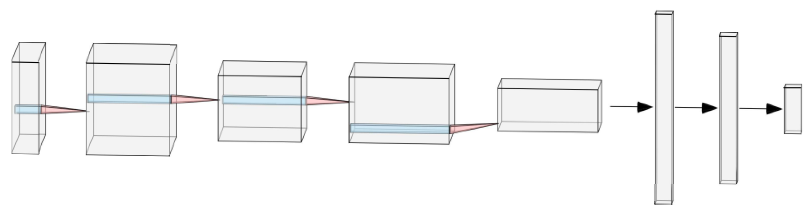
Table 3. CNN architecture.
LayerConvolution
Kernel Size
Step of
Convolution
Kernel
Number of
Convolution
Kernels
Output SizeWeightParameters
Convolution3 × 323264 × 48 × 323 × 3 × 1 × 32896
Pooling3 × 323222 × 16 × 32//
Convolution3 × 316422 × 16 × 643 × 3 × 32 × 6418,496
Pooling3 × 31648 × 6 × 64//
FC///1 × 1 × 30723072 × 40961,573,376
FC///1 × 1 × 512512 × 307265,664
Output///1 × 1 × 7/903
Table 4. Identification of the fault status for traveling valve leakage.
LabelDynamometer CardRelated VectorsThe Variation of
Characteristic Parameters
Output of CNNOutput of
Expert Rules
Result
Traveling valve leakageEnergies 16 03170 i001[0.0, 0.0, 0.003,…,
0.009, 0.003, 0.0]
/[0.0873,
0.0006,
0.8107
0.0023,
0.0001,
0.0154,
0.0836]
Traveling valve
leakage
(Confidence: 0.5)
Traveling valve leakage
[52.55, 53.13, 54.35,…,
52.49, 52.58, 52.52]
/
[80.6, 80.54, 80.78,…,
77.11, 76.96, 77.14]
−0.03
[54.15, 54.62, 54.0,…,
49.81, 49.87, 49.99]
0.03
[110.5, 111.39, 111.49,…,
44.72, 43.71, 43.91]
−0.27
[26.45, 25.92, 26.78,…,
27.3, 27.09, 27.15]
0.08
Table 5. Identification of the fault status for standing valve leakage.
LabelDynamometer CardRelated VectorsThe Variation of
Characteristic Parameters
Output of CNNOutput of
Expert Rules
Result
Standing valve leakageEnergies 16 03170 i002[0.0, 0.0, 0.0,…,
0.006, 0.003, 0.0]
/[0.0001,
0.0138,
0.0146, 0.9582,
0.0131,
0.0002,
0.0000]
Standing
valve leakage
(Confidence: 0.5)
Standing valve leakage
[61.91, 63.13, 64.43,…,
57.66, 59.23, 60.79]
/
[83.14, 83.26, 83.66,…,
79.62, 79.73, 80.02]
−0.05
[41.96, 42.01, 41.27,…,
47.86, 47.83, 47.6]
−0.08
[150.89, 151.77, 157.82,…,
107.5, 109.43, 110.69]
−0.12
[41.18, 41.28, 42.39,…,
31.76, 31.9, 32.42]
−0.06
Table 6. Identification of the fault status for sudden sucker rod break.
LabelDynamometer CardRelated VectorsThe Variation of
Characteristic Parameters
Output of CNNOutput of
Expert Rules
Result
Sudden sucker rod breakEnergies 16 03170 i003[0.0, 0.01, 0.019,…,
0.007, 0.007, 0.003]
/[0.1024,
0.0002,
0.0528,
0.0000,
0.5533,
0.0001,
0.2914]
Sudden
sucker rod break
(Confidence: 0.8)
Sudden sucker rod break
[51.79, 52.0, 52.06,…,
51.2, 51.32, 51.55]
/
[73.69, 73.75, 73.66,…,
74.35, 52.89, 52.6]
−0.27
[59.49, 59.46, 59.28,…,
58.45, 51.2, 50.63]
−0.05
[28.54, 28.33, 28.15,…,
20.58, 4.86, 6.14]
−0.89
[14.2, 14.29, 14.38,…,
15.9, 1.78, 1.97]
−0.81
Table 7. Identification of the fault status for paraffin deposition.
LabelDynamometer CardRelated VectorsThe Variation of
Characteristic Parameters
Output of CNNOutput of
Expert Rules
Result
Paraffin depositionEnergies 16 03170 i004[0.0, 0.005, 0.005,…,
0.014, 0.0, 0.0]
/[0.2921,
0.3180,
0.0044,
0.0873,
0.0008,
0.2045,
0.0929]
Paraffin deposition (Confidence: 0.7)Paraffin deposition
[53.15, 54.65, 56.3,…,
51.44, 51.7, 52.18]
/
[87.31, 87.49, 87.28,…,
93.47, 91.64, 93.44]
0.06
[53.29, 53.53, 53.71,…,
46.45, 47.37, 47.39]
−0.18
[80.79, 74.91, 81.24,…,
121.63, 126.87, 125.77]
0.82
[34.02, 33.96, 33.57,…,
47.02, 44.27, 46.05]
0.24
Table 8. Identification of the fault status for pumping with gushing.
LabelDynamometer CardRelated VectorsThe Variation of
Characteristic Parameters
Output of CNNOutput of
Expert Rules
Result
Pumping
with gushing
Energies 16 03170 i005[0.0, 0.004, 0.02,…,
0.055, 0.026, 0.004]
/[0.0137,
0.0158,
0.0966,
0.0000,
0.1775,
0.0791,
0.6173]
Pumping
with gushing
(Confidence: 0.9)
Pumping
with
gushing
[34.19, 35.04, 35.23,…,
31.83, 32.33, 33.16]
/
[35.13, 35.13, 35.02,…,
35.11, 35.13, 35.23]
0.01
[28.44, 28.46, 28.55,…,
28.46, 28.58, 28.58]
−0.01
[19.85, 19.71, 19.6,…,
19.93, 19.71, 20.04]
−0.04
[6.69, 6.67, 6.47,…,
6.65, 6.55, 6.65]
−0.05
Table 9. Fault status diagnosis results.
Fault CategoryNumber of SamplesCNN AccuracyHybrid Accuracy
Normal35894.12%/
Insufficient liquid supply107194.44%/
Traveling valve leakage9666.66%88.89%
Standing valve leakage7171.43%85.71%
Sudden sucker rod break38578.95%100%
Paraffin deposition5572.73%100%
Pumping with gushing3080.00%100%
All206676.25%97.50%
Disclaimer/Publisher’s Note: The statements, opinions and data contained in all publications are solely those of the individual author(s) and contributor(s) and not of MDPI and/or the editor(s). MDPI and/or the editor(s) disclaim responsibility for any injury to people or property resulting from any ideas, methods, instructions or products referred to in the content.

