Determination of Thermocline Heat Transfer Coefficient by Using CFD Simulation

Abstract

This article deals with a thermal energy storage system in the form of a water tank with a thermocline. The well-known thermocline phenomenon is modeled using computational fluid dynamics (CFD). However, the reservoir model proposed in this article is zero-dimensional. This is due to the fact that the aim of this article is to build a mathematical model that will be more useful in mathematical models of complex energy systems in which a hot water tank is one of many elements of the system. In such a zero-dimensional mathematical model, the hot water tank will be modeled using equations describing heat transfer, and the thermocline itself will be treated as a heat transfer surface with known dimensions and heat transfer coefficient. A novelty of this paper is that it addresses heat loss across the thermocline as defined in this manner. A CFD model of a thermal storage tank is created, validated with available experimental data, and used to obtain the heat transfer coefficient U. The resulting value is then analyzed quantitatively and qualitatively and the changes in the thickness of the thermocline are accounted for in the equation. The results from this groundbreaking work can be used to analyze heat storage in the form of thermocline water tanks at the level of system modeling, e.g., for the purpose of configuring the structure of other devices and control systems.

1. Introduction

Energy storage requirements are rising in tandem with the ever-increasing share of renewables in the energy mix. Development of electrical energy storage technologies and methods is constantly moving ahead [1,2,3]. Thermal energy storage research is not attracting the same intensity of interest [4], despite a common oversupply of thermal energy from solar panels in summer which, logically, could be stored for the heating period. Set out below is a brief overview of current storage solutions, predominantly based on thermocline water tanks with differing degrees of insulation against heat loss to the environment. However, there are still losses resulting from the transport of heat directly via the thermocline.

Several research works have focused on mathematical modeling of hot water storage tanks. The authors of [5] described the results of a three-dimensional, transient CFD (Computational Fluid Dynamics) [6,7] mathematical model for various designs of hot water storage tanks and various operating parameters. The model was used to investigate the influence of various configurations on the flows, stratification, and performance of storage tanks in solar power systems.

The thermal conductivity of the inner lining material also affects the stratification phenomenon inside the hot water tank during tank loading and then during the heat storage period, which was investigated in [8]. Numerical studies of the three-dimensional CFD model of the tank were carried out. The mathematical model was validated through experimental studies of temperature profiles inside the tank as a function of time.

The authors of [9] described improvements to the SpiralSol program used to calculate the performance of domestic hot water tanks. The program was improved with intra-reservoir stratification modeling. For this purpose, CFD modeling was used to determine fluid flow and heat transfer inside the tank during cooling caused by heat losses.

CFD analysis of the stratification occurring in a domestic hot water tank during dynamic operation is shown in [10]. It showed the thermal behavior in a vertical hot water tank based on a model built in Fluent v6.3. Literature experimental data were used to validate the model.

The simulation results of charging and discharging cycles showed thermal stratification and characteristics of flow. The Richardson number and stratification efficiency were calculated.

In [11], thermal stratification in a hot water tank with an inner cylinder was investigated using CFD methods. The influence of inner cylinder design and operating parameters on the flow characteristics, thermal stratification, and overall performance during tank loading was investigated.

Experimental studies and a series of CFD simulations of a horizontally positioned hot water storage tank are described in [12]. This tank is an element of a prototype solar absorber with evacuated tube collectors comprising heat pipes. Thermal imaging was used during the experiments to determine the maximum temperatures of the heat pipes.

CFD methods to test the operation of a hot water tank with an internal heat exchanger were reported in [13]. The work proposed changing the geometry of the reservoir to improve its stratification properties. The proposal was to have an additional smaller vessel, fitted with a heat exchanger, to improve stratification formation in the larger vessel.

A review of solar energy storage technologies based on hot water storage tanks using stratification is contained in [14]. The review features mathematical equations for modeling thermal stratification and performance indicators for evaluating hot water storage tanks.

Research on a hot water tank with an immersed layer of balls with PCM (phase-change material) is reported in [15]. Stratification occurred during operation, experimental research was conducted, and a CFD model was built. The influence of PCM on the properties of the hot water tank was investigated.

Simulations of thermal stratification in hot water tanks were carried out by a research team and described in [16]. Stratification was investigated both experimentally and numerically during cooling, when the tank was neither loaded nor unloaded.

The validated model was two-dimensional. The results showed that natural convection takes place mainly at the top of the tank and forms a boundary layer along the walls that guides the cooled water downwards.

Ref. [17] presents numerical and experimental studies of stratification inside a hot water tank.

The influence of placing flat surfaces inside the tank on the operation of the tank was also examined. Good results were obtained for a flat surface placed in the center of the hot water tank and it was also found that placing flat surfaces at different angles in certain configurations improved thermocline formation.

In [18], a mathematical model of a hot water tank using the phenomenon of stratification was presented and validated. The novelty of that model was to use a continuous and smooth function for modeling the dynamics of mixing and buoyancy.

An overview of various solutions regarding the phenomenon of stratification in domestic hot water tanks is presented in [19]. This review included, among others, a multi-node solution and plug flow approach to model the temperature distribution. Temperature distribution models were divided into: linear, stepped, continuous–linear, and three-zone.

In [20], the influence on stratification of the cold-water supply method during discharge of a domestic hot water tank was investigated. Several methods of supplying cold water were tested. CFD models were built for the tested tank geometry and different geometries of cold-water inlets.

The process of thermocline behavior during charging of a thermal energy storage vessel was analyzed in [21] where researchers precisely modeled thermocline thickness using Ansys-Fluent software and proposed a method for the quantification of thermocline thickness.

In [22], the influence of a baffle plate with a central hole on thermal stratification inside the hot water tank was analyzed. The parameters of this design were optimized with response surface methodology. The characteristics of thermal stratification were investigated experimentally and a three-dimensional transient CFD mathematical model was built.

A rather unusual hot water tank solution was presented in [23]. There, numerical and experimental tests were carried out on a hot water storage tank with a mantle heat exchanger, a configuration commonly used in balcony solar water heating systems in China.

Operation of thermocline-based single media tanks for the needs of a solar power plant with concentrators is described in [24]. The influence of various parameters on the thickness of the thermocline was analyzed there. Comsol Multiphysics software was used to build a mathematical model. The results showed that the thickness of the thermocline can be reduced by using a vertical porous flow distributor inside the tank.

The thermocline can also be obtained not only in systems filled with water. In [25], the operation of a tank with a packed bed for heat storage for the needs of a solar power plant based on the technology of solar concentrators was analyzed. Temperature profiles for a tank filled with porous solid materials flowed by various commercial Heat Transfer Fluids (Therminol, HITEC, Solar Salt) were shown.

Novelty

The available literature contains numerous experimental and numerical studies on stratified storage tanks with various methods to assess thermal stratification in water tanks. Fertahi et al. [14] reported how various indicators are used to assess the performance of thermal stratification such as stratification number, MIX number, and Richardson number. However, for our further study, i.e., system-level modeling and optimization of seasonal thermal energy storage system [26], we need a 0D relationship for the loss through the thermocline, which could be implemented for software such as Hysys, TRNSYS, and Ebsilon.

The paper introduces the 0D formula for heat transfer through the thermocline, which was derived based on a CFD simulation validated against available experimental data. The equation is useful for system-level modeling (e.g., our study [26]) for simulations which include the phenomena of heat transfer through the thermocline. Most work to date has ignored these losses, focusing only on losses through insulation to the environment. Thus, what is new is the development of a relationship that we believe may be useful to other researchers through its implication in other 0D models (e.g., TRNSYS).

2. Methods

The research methodology is based on development of a CFD model of a hot water tank. The main assumptions for modeling are described in Section 2.1 Model development. Furthermore, the model was verified against experimental data (see Section 2.2 Model validation) section. The simulation results were used to derive a mathematical function for heat loss through thermocline.

2.1. Model Development

The geometry of the tank was created in Ansys SpaceClaim. The axisymmetric flow domain was utilized to reduce the problem to the 2D plane, with the axis boundary condition in the centerline of the tank geometry. Boussinesq approximation was used to model density variation due to changing temperature, which is necessary in convective flow simulations.

The simulations were prepared with reference to the Ansys FLUENT Theory Guide to deliver the best possible solution convergence. The general energy equation underscoring the simulations encompasses most of the described energy transfer effects, according to the following equation:

$$\frac{\partial }{\partial t}\left(\rho E\right)+\nabla ·\left(\overrightarrow{\upsilon }\left(\rho E+p\right)\right)=\nabla ·\left(k_{eff}\nabla T-{{\displaystyle \sum }}_j{h}_j\overrightarrow{J_J}+\left({\stackrel{=}{\tau }}_{eff}·\overrightarrow{\upsilon }\right)\right)+S_h$$

(1)

where $k_{eff}$ describes conductivity including turbulent conductivity, according to the turbulence model that was used in the simulations. Parameter $\overrightarrow{J_J}$ represents diffusion flux of species j. The three terms in the brackets on the right side of the equation describe energy transfer due to: conduction ($k_{eff}\nabla T$), species diffusion (${\displaystyle \sum }_j{h}_j\overrightarrow{J_J}$), and viscous dissipation $\left({\stackrel{=}{\tau }}_{eff}·\overrightarrow{\upsilon }\right)$. The final part of the equation ($S_h$) indicates heat occurring due to chemical reactions or other heat delivered by volumetric sources; this and species diffusion are irrelevant in the analyzed case, as only one agent was used.

Three fluid zones have been created in the developed tank model. Two fluid zones, one for upper half of the tank and one for lower half, and a solid zone for the wall and insulation of the tank. Thermoclines are strictly dependent on the density of the fluid; the density–temperature relationship was in the form of the Boussinesq model, which generally allows for natural convection arising from small changes in temperature. Large temperature differences trigger problems related to combustion, reacting flows, and species calculations. Water is the agent used in the designed installation, with the temperature difference being approximately 40 K. The material parameters used for the simulations are presented in

Table 1. Material parameters of the agent (water) applied for the simulations and operating conditions for calculating natural convection.

Properties	Unit	Value	Function
Density	kg/m3	992.25	Boussinesq
Cp (Specific Heat)	J/kg-K	4182	constant
Thermal Conductivity	W/m-K	0.6	constant
Viscosity	kg/m-s	0.001003	constant
Molecular Weight	kg/kmol	18.0152	constant
Thermal Expansion Coefficient	K−1	6.9 × 10−0.5	constant
Standard State Enthalpy	J/kgmol	−2.858 × 108	constant
Standard State Entropy	J/kgmol K	69,902.21	constant
Reference Temperature	K	298	constant
L-J Characteristic Length	Angstrom	1	constant
L-J Energy Parameter	K	100	constant
Latent Heat	J/kg	2,263,073	constant
Vaporization Temperature	K	284	constant
Boiling Point	K	373	constant
Binary Diffusivity	m2/s		film-averaged
Droplet Surface Tension	N/m	0.0719404	constant
Gravitational Acceleration	m/s2	9.81 (Y axis)	constant
Operating Temperature	K	333	constant
Operating Density	Kg/m3	992.25	Boussinesq

.

The following boundary conditions have been applied to the model in ANSYS Fluent in order to perform calculations. In the Y-axis, the acceleration due to gravity was set to 9.81 m s⁻². The operating temperature was set at 333 K, the mid-point between the temperatures of the upper and lower regions of the tank. Heat loss to the environment has been solved with use of thermal boundary conditions: temperature equal to 300 K, convection-free stream temperature equal to 300 K, and radiation-external radiation temperature equal to 300 K.

The Bussinesq model allows for quick convergence of the simulation by making the density dependent on the temperature. A constant density value has been used in almost all equations. The exception was the impact of buoyancy on the solution defined in the momentum equation:

$$\left(\rho -{\rho }_0\right)g\cong -{\rho }_0\beta \left(T-T_0\right)g$$

(2)

where $T_0$ represents operating temperature, $\beta$ defines the coefficient of thermal expansion, and ${\rho }_0$ is the flow density constant. The equation above is obtained with the Boussinesq approximation $\rho ={\rho }_0\left(1-\beta ∆T\right)$ for the elimination of $\rho$ in the buoyancy term, and it can be used when changes in actual density of the agent are small, namely when $\beta \left(T-T_0\right)\ll 1$.

Interpolation for the discretization was performed using PRESTO! (Pressure Staggering Option), which utilizes the discrete continuity balance for “staggered” control pressure, enabling calculations to be made for zones with pressure gradients [27,28].

2.2. Model Validation

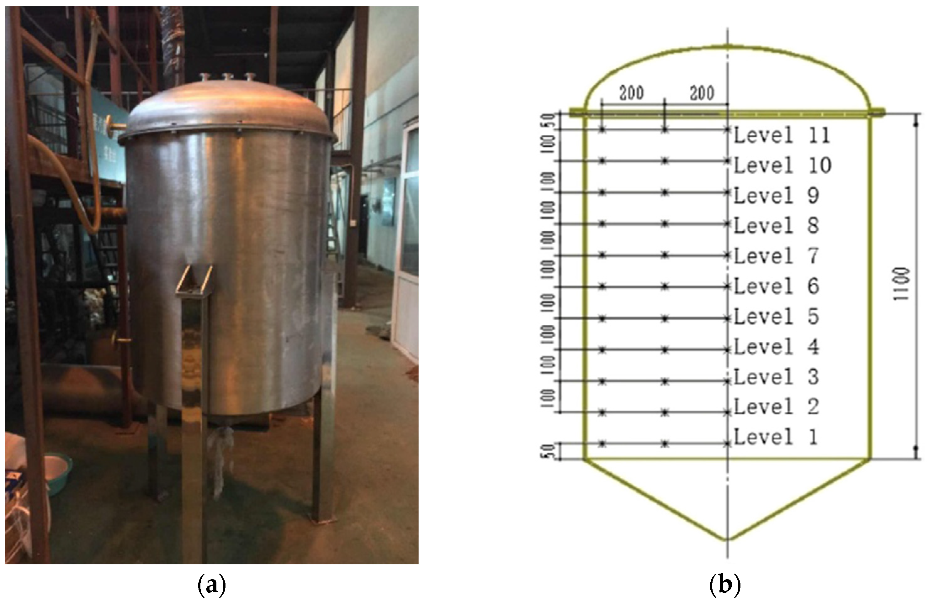
The view of tank, which was a source of experimental data is shown in Figure 1a. The authors in [29] measured the temperature inside the tank using 33 K-thermocouples, which were located in 11 levels (3 thermocouples per each level). The distribution of thermocouples inside the experimental tank are shown in Figure 1b. He et al. [29] insulated the vessel by adding a 25 mm asbestos insulation layer.

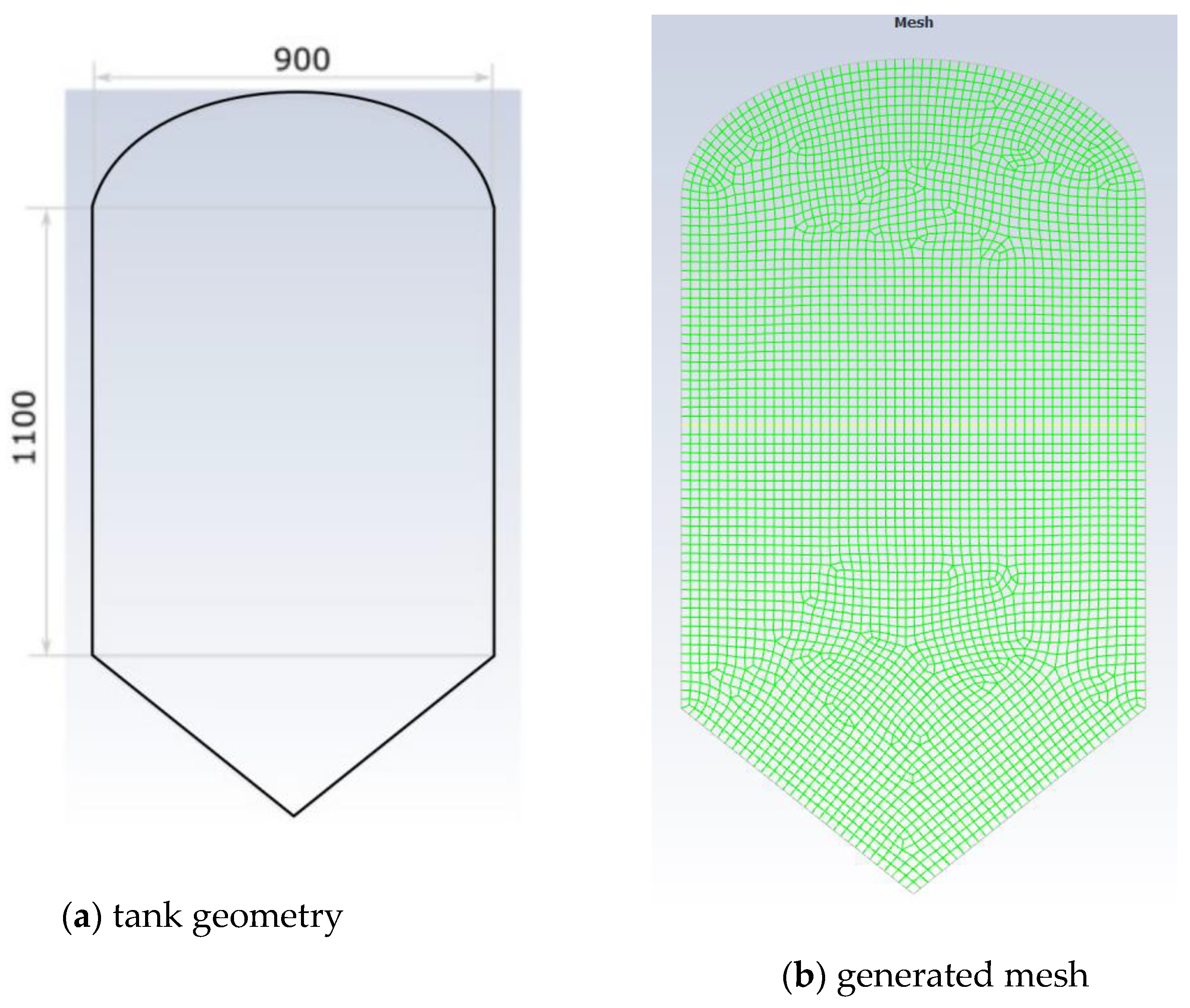
Using the Ansys SpaceClaim program, the geometry of the modeled tank was built, the experimental studies of which come from [29]. This geometry (in 2D) is shown in Figure 2a. The presented model also includes heat losses outside the tank through a 5 mm tank wall and 25 mm insulation. Based on the presented geometry, a mesh was built using Ansys Design and the edges specification was established to set the boundary conditions. It was set so that the largest element inside the tank could be 10 mm. In turn, in the case of the tank wall, the maximum element could be 1 mm, and in the case of insulation—5 mm. Figure 2b shows the mesh that takes into account the assumptions described above.

As our simulation aims to derivate a 0D formula, we decided to opt for heat loss through the thermocline. Thus, we created mesh using default settings and we compared results with the experimental data. As both the simulation time and simulation results was satisfactory, we decided not to provide the mesh sensitivity as in the article of Hosseinia [21].

For the simulation, we assumed that the thermal conductivity of the wall (made of steel) is 45 W/mK and the same parameter of the insulation (made of asbestos) is 0.18 W/mK.

The other parameters of materials from which the modeled system is built are listed in

Table 2. Parameters of materials from which the modeled system is built.

Material	Density, kg/m3	Average Specific Heat (at 20 °C)	Thermal Conductivity
	r kg/m3	Cm kJ/kgK	λ W/mK	t °C
Aluminum foil with 10 mm air layer	3.6	-	0.03 0.056	0 300
Aluminum foil with 16 mm air layer	3.6	-	0.04 0.086	0 300
Asbestos	140	0.796	0.05	20

.

At the beginning of the calculations, the thermocline was located in the middle of the tank height. The calculations were started according to the data from [29], which meant that the temperature at the top of the tank was 353 K and at the bottom it was 313 K.

The time step was selected at the level of 5 s. A higher value of the time step results in a decrease in the convergence of calculations with experimental data and a rapid disappearance of the thermocline. Every 60 time steps (every 5 min) the temperature profile in the tank axis was exported automatically, thanks to which it was possible to create graphs of the temperature distribution in the thermocline over time. In order to determine the heat flux through the water and the walls of the tank, average temperatures from the upper and lower zones in the tank were saved.

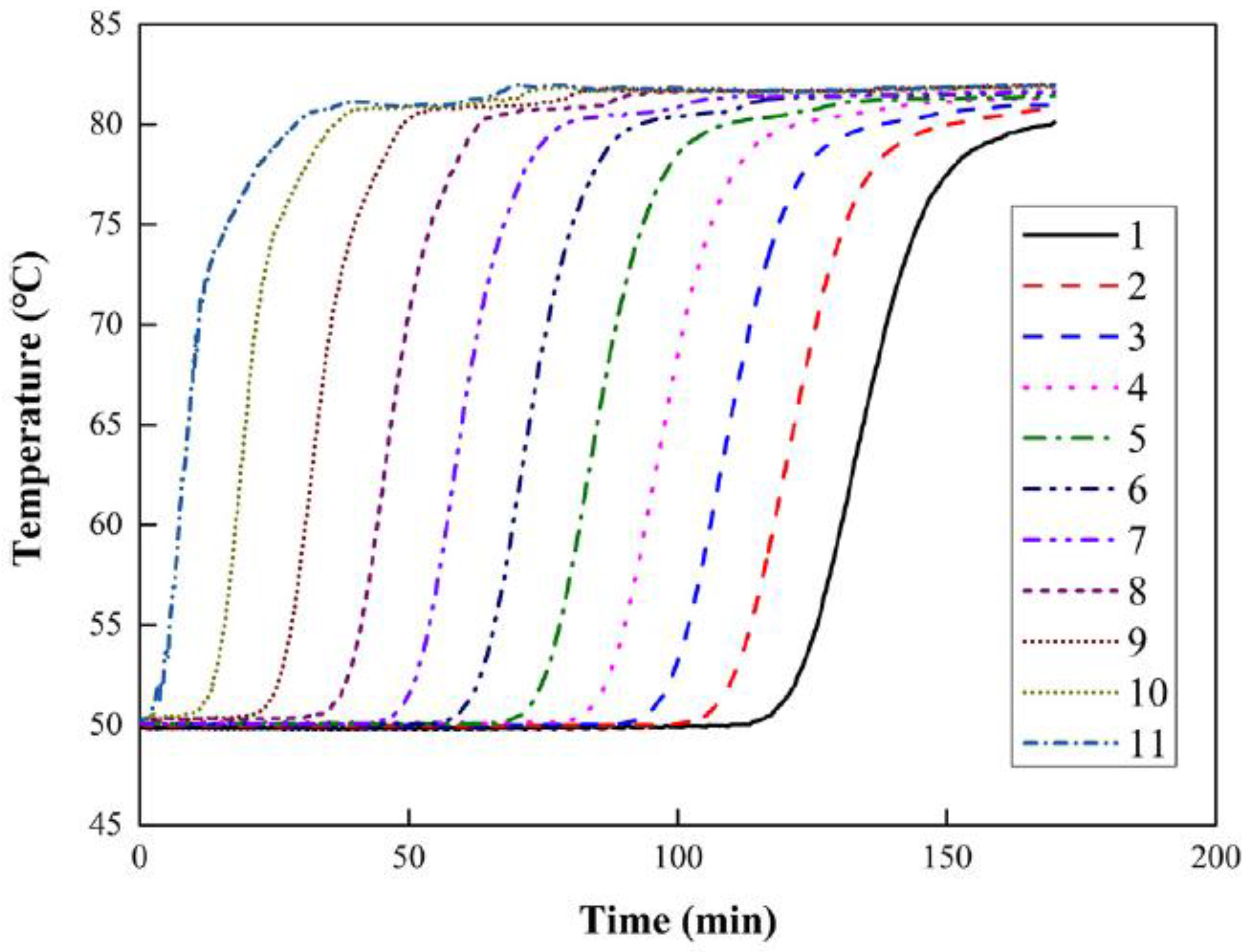
The changes in the temperature profile in the vertical axis of the tank over time are shown in Figure 3. The thermocouples placed in the actual tank were numbered (from bottom to top) from 1 to 11. The last (11th) thermocouple is the first to register a temperature change due to its proximity to the tank filling location and non-laminar flow and hot- and cold-water mixing. When filling the tank, the most irregular temperature distribution was observed between 25 and 45 min. This effect was reduced for thermocouples located lower (further from the filling point). For example, for thermocouples 1 to 7, this effect was barely noticeable. It can therefore be said that during the tank loading process, the influence of non-laminar flow disappears below one third of the tank (counting from the top).

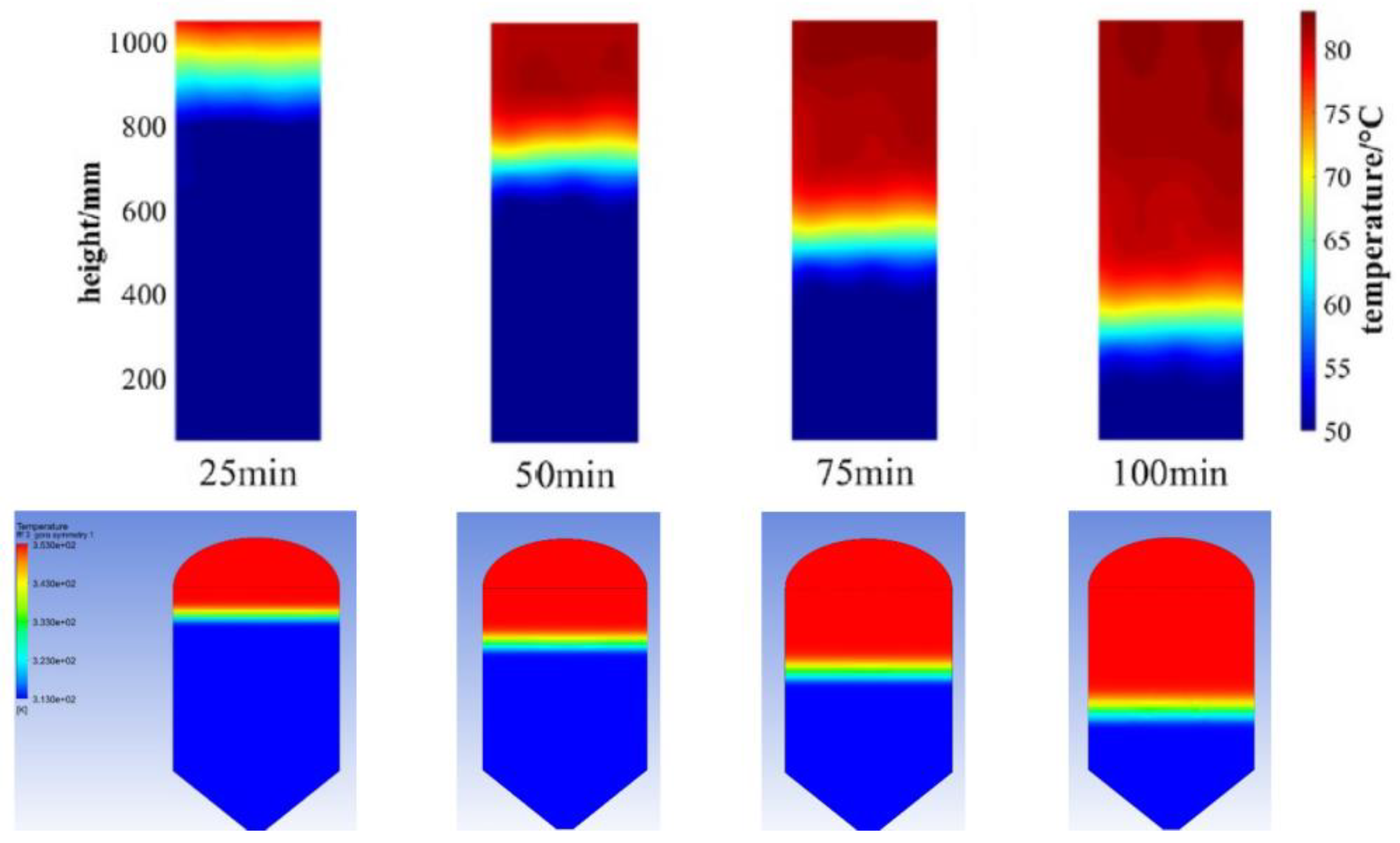
The level of the thermocline defined by the model as a function of time was similar to the level of the thermocline measured during experiments when the tank was filled with hot water. The experimental and modeling results are compared in Figure 4.

The comparison of the simulation results and the experimental data brought us to the conclusion that the model is reliable and can be used as a tool for further investigations.

3. Determination of Heat Transfer Coefficient through the Thermocline

A hot water tank model built based on CFD calculations was used to determine the heat losses through the thermocline (see Figure 5). Thanks to this, it was possible to determine an equation that could then be used in 0D models such as Aspen HYSYS for dynamic calculations of entire systems comprising heat storage based on a thermocline.

The model of the heat storage tank constructed in this way was three-dimensional and contained a zone of cold and hot water and a thermocline between them. This model was used to derive the formula for heat loss through the thermocline. In order to enable this, the possibility of heat exchange with the environment was blocked in this model. As a result of these treatments, heat exchange was possible only through the thermocline and along the walls of the tank, conducting heat from the hot zone to the cold zone of the tank. The modified model was again used to simulate the operation of the tank for a month. At the start of such a simulation, the temperature on the hot side was 80 °C and on the cold side it was 40 °C (see Figure 6).

The following equation can be used as a starting point to describe heat transfer through a thermocline:

$$Q_{h\to l}=A\cdot U\cdot \Delta T$$

(3)

where $U$ is the coefficient of heat transfer; W/m²/K; A is the heat transfer surface area, which here means the surface area of thermocline, m²; and $\Delta T$ is the temperature difference between the lower and upper sides of the thermocline: $\Delta T=t_h-t_l$.

The amount of heat that is exchanged can also be determined by changes in temperature over time:

$$Q_{h\to l}=\frac{\left(t_{h,{\tau }_0}-t_{h,{\tau }_1}\right)\cdot c_v\cdot V_h\cdot {\rho }_{water}}{{\tau }_1-{\tau }_0}$$

(4)

where $\tau$ is the time step, seconds; t is the temperature, K; c_v is the specific heat of water; $\rho$ is the density of water, kg/m³; and V is the volume of hot space in the vessel, m³.

As a result of substituting Equation (3) into Equation (4), we obtain the following equation describing the heat transfer coefficient U:

$$U\left({\tau }_1\right)=\frac{\left(t_{h,{\tau }_0}-t_{h,{\tau }_1}\right)\cdot c_v\cdot V_h\cdot {\rho }_{water}}{\left({\tau }_1-{\tau }_0\right)\cdot \left(t_{h,{\tau }_0}-t_{l,{\tau }_0}\right)\cdot A}$$

(5)

This equation was used to determine the value of the heat transfer coefficient U during the erosion of the thermocline, and the results obtained in this way are shown in Figure 7. The arithmetic mean for the resulting set of data was 0.193 W/m²/K.

At the outset, it should be clarified that the occurrence of negative U-values may be the result of heat accumulation by the walls of the hot water reservoir as a result of stopping heat exchange with the environment. Determining the temperatures on both sides of the thermocline is also not an obvious issue, due to the fact that the thermocline has no clear boundaries. Therefore, the temperatures on both sides of the thermocline can be obtained by averaging, which can also be used to determine the operating parameters for a zero-dimensional model of a hot water tank.

$$U=0.193 \mathrm{W}/{\mathrm{m}}^2/\mathrm{K}$$

(6)

4. Discussion

The goal of this study was to compare the insulation properties of a thermocline with other materials. To that end, its thickness must be determined. The temperature distribution of the medium in the tank was analyzed and the height of the tank at which sudden temperature changes occur was determined. The analysis of the temperature distribution, together with an indication of the thermocline, is shown in Figure 8.

The thickness of the thermocline in the analyzed case was assumed to be 132 mm. As an alternative to a thermocline, a physical barrier made of insulating material could provide thermal insulation between the hot and cold water. Three different insulation materials were considered, and their thermal conductivity properties are summarized in

Table 3. Thermal conductivity of selected materials.

	Thermal Conductivity, W/(mK)
Water	0.61
Asbestos	0.11
Styrodur	0.04
PU foam	0.03

. The thickness of the thermocline is somewhat of an arbitrary parameter, and over time the thermocline disappears, so its maintenance is possible by frequent charging and discharging of the heat storage tank. We studied dynamic states, so that at any moment in time it was possible to determine the temperature distribution along the tank, which generally speaking is similar in shape to the hyperbolic tangent. By running a straight line through the tagh(0) it is possible to find the points of intersection between this line and the tagh(+/infinity) lines, which determines the thickness of the thermocline in our case (refer to Figure 8). The tank being tested was loaded/unloaded relatively quickly, so changes in thermocline thickness were not significant. In the future, we plan to develop the model to include the effect of time on thermocline thickness, once we have test results from our installation and not just from literature data. It should be mentioned, however, that the driving factor for heat loss through the thermocline is the temperature difference above and below the thermocline, so that changes in its thickness over time do not have a significant effect. As far as the hypothetical heat transfer coefficient is concerned, it was compared with other insulation materials to better illustrate the value we obtained.

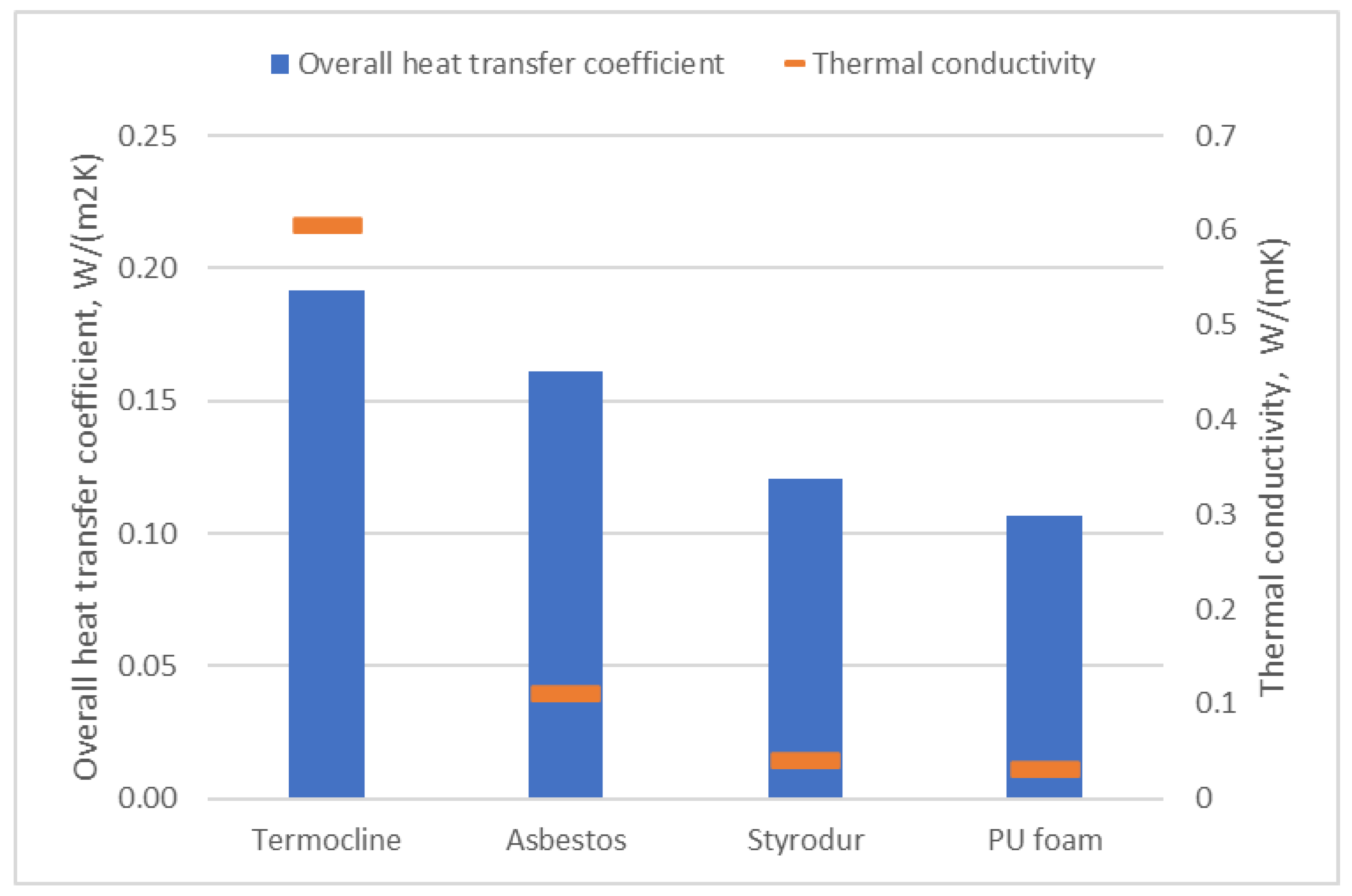
These insulating materials have significantly better insulating properties than water. To determine how the value of the overall heat transfer coefficient between water layers would change, simulations of the influence of the stated physical layers on this coefficient were conducted. The calculations assumed equal thickness of the thermocline and physical layer. The results are presented in Figure 9.

If the exact value of the heat transfer coefficient was maintained, the thickness of the physical layer made of the various individual materials would be noticeably thinner than the thermocline (see

Table 4. Thickness of the layers of insulating materials corresponding to the thermocline.

	Thickness, cm
Asbestos	2
Styrodur	0.8
PU foam	0.6

). However, a tank with a mobile physical insulating layer would be significantly more complicated in terms of manufacturing and this would impact reliability.

5. Conclusions

The motivation for this work was to find the heat transfer coefficient of a thermocline in a water tank. Whereas a complete three-dimensional model would evidently yield more accurate results, there are cases in which either the geometry is unknown or is still to be determined by calculation. Such cases concern 0D models for the calculation of entire systems and selection of control systems. While it is far more convenient in such cases to use known heat transfer equations, the problem lies in determining the amount of heat transferred, which depends on the temperature difference and the thermocline surface area.

A 3D model was built to simulate the behavior of a hot water tank for which another research team had previously published experimental data. The model was verified on this basis. Heat exchange with the environment was eliminated and the process of thermocline decay as a result of temperature equalization in the reservoir was simulated. The results obtained from the CFD model were used to track temperature changes in the lower and upper volumes of the tank.

In order to describe the heat transfer through the thermocline, the formula for the heat transfer coefficient U between its upper and lower sides was derived and then the value of this coefficient was calculated. By relating the heat transfer through the thermocline with temperature changes over time, the average value of the U coefficient was obtained for the considered time period (1 month). The obtained thermocline U value was then compared with commonly used insulation materials.

The article deals with an attempt to use CFD calculations to derive a 0D relationship for heat loss through the thermocline, which was applied to a dynamic model of a seasonal heat storage tank. We believe that this relationship will be useful to other researchers wishing to take these heat losses into account in their simulations. Most work to date has ignored these losses, focusing only on losses through insulation to the environment. Thus, what is new is the development of a relationship that we believe may be useful to other researchers through its implication in other 0D models (e.g., TRNSYS). The obtained equation does not look impressive, but it has nevertheless been obtained after many tedious and lengthy calculations of a real tank containing a thermocline. The resulting relationship does not relate to different points in time, but rather is a relationship based on average data, with temperatures at the same point in time inserted into the calculation. This relationship models heat loss through the thermocline, which is generally not included in other models, so it has great cognitive value despite its simplicity.