Evaluation of Operation State of Power Grid Based on Random Matrix Theory and Qualitative Trend Analysis

Abstract

Bulk power grid interconnection and the access of various smart devices make the current grid highly complex. Timely and accurately identifying the power grid operation state is crucial for monitoring the operation stability of the power grid. For this purpose, an evaluation method of the power grid operation state based on random matrix theory and qualitative trend analysis is proposed. This method constructs two evaluation indicators based on the operation data of the power grid, which cannot only find out whether the current state of the power grid is stable but can also find out whether there is a bad operation trend in the current power grid. Compared with the traditional method, this method analyzes the power grid’s operation state from the big data perspective. It does not need to consider the complex network structure and operation mechanism of the actual power grid. Finally, the effectiveness and feasibility of the method are verified by the simulations of the IEEE 118-bus system.

1. Introduction

In recent years, with the continuous development of smart grid, the scale of the current power system has become more and more monumental. The increasingly complex operating characteristics make the potential problems of power grid operation more prominent [1,2,3,4]. How to quickly and accurately assess the operation state of the power grid is a significant problem today.

At the same time, as more intelligent devices have been connected to the power system, the grid has stored massive and high-dimensional operational data during the operation [5,6]. These data have the characteristics of 4Vs [7,8], which contain rich and valuable information and are closely related to the stable operation of the power system [9,10,11].

Exploiting the value of these electric power big data has become important research content for current researchers. At present, the general research idea of using data to analyze power system operation in power system stability analysis is to establish indicators of power grid operation state from different perspectives, respectively, and then to evaluate the system comprehensively by fuzzy comprehensive evaluation method [12], analytic hierarchy process (AHP) [13], entropy theory [14] and so on. For example, in [15], the authors first constructed the operational indicators of the distribution network from three aspects: system operational risk, PV generation uncertainty and network topology robustness; they then used the improved analytic hierarchy process (IAHP) to calculate the weights of different indicators; finally, they summed up to obtain the operational safety indicators of the distribution network. The accuracy of this comprehensive assessment method to evaluate the operation state of the grid is highly dependent on the established indicators system, so this method is not widely applicable.

Random matrix theory (RMT) is a data analysis method specifically designed to work with high-dimensional data [16,17]. Like deep learning, RMT is also a very effective data analysis tool at present. Both of them have unique advantages in high-dimensional space: the RMT has flexible and rigorous mathematical analysis capabilities, and the deep learning has superior data modeling capabilities. Deep learning technology in engineering applications usually requires labels and has specific requirements on the categories and quantity of labels. But the data sets in the actual power grid often find it difficult to meet the above conditions. RMT does not need to define labels, and there is no model training as complex as deep learning; so it is more efficient and suitable for dealing with complex power grids with complex models, strong uncertainty, unclear causality and high data dimension. In [18], random matrix theory was first introduced into the field of power systems. Subsequently, in [19], a correlation analysis method based on random matrix theory was proposed, which can analyze the connection between various factors and grid operation state in real-time and quantitatively. In [20], a method for analyzing and locating system anomalies and disturbances based on random matrix theory was proposed. In [21], for the distribution grid with high penetration of renewable energy with a high uncertainty problem, the authors proposed a topology identification method using random matrix theory to improve the effectiveness of topology identification. In [22], a method which can effectively identify the abnormal state of power consumption by random matrix theory was proposed. In [23], based on random matrix theory, a data-driven approach for fault time determination and fault area location to avoid the influence of bad data was proposed. In [24,25], the authors used the big data fusion technology of random matrix theory to evaluate the static stability and transient stability of the power grid, ignoring the complex physical model and making full use of the high-dimensional and massive data generated during operation. These above studies show the excellent applicability of random matrix theory for analyzing the operation state of the power grid.

For a power grid in operation, the causes of faults during grid operation usually can be divided into two types: sudden faults and deterioration of poor operating conditions. Identifying the former is relatively easy while identifying the latter is more difficult. If we want to detect the deterioration of the state during the power grid operation, we must analyze the trend of the grid operation and observe whether the current trend of the grid operation is getting better or worse. Therefore, it is also essential to focus on trends when assessing the stable operation of the grid. As a special method to study the trend of data change, trend analysis is a crucial part of data analysis [26,27]. It effectively identifies essential information embedded in the data and is now widely used for process monitoring and fault diagnosis [28,29]. In [29], the authors state that using trend analysis techniques to analyze data’s operational trends can help operators monitor and identify potential problems.

Therefore, this paper uses a qualitative trend analysis technique based on the random matrix theory to evaluate the current grid operation state and the trend of state change for two causes of faults. Firstly, a random matrix model that characterizes the operating state of the power grid is built using historical data and current real-time data. Secondly, based on the Marcenko-Pastur(M-P) law and ring law of random matrix theory, two indicators are defined to evaluate the current stable operation state of the power grid. Thirdly, compare two indicators, and determine the more suitable indicator to reflect the integrity of the system according to the characteristics of the two indicators. Fourthly, the qualitative trend analysis technique is used to analyze the indicator sequence that can show the integrity of the system. Its trend represents the trend of the power grid operation state. By analyzing the trend change of the indicator, we can judge whether there is a bad trend affecting the stable operation of the current power grid and realize the effective monitoring of the operation state of the power grid. Finally, the effectiveness and feasibility of the proposed method are verified by simulations based on IEEE 118-bus test system.

The rest of the paper is as follows: Section 2 introduces the random matrix theory and matrix model based on grid operation data. Section 3 introduces the qualitative trend analysis techniques. Section 4 shows the process of real-time grid operation state assessment. Section 5 contains two examples and discussions of the results. Finally, the full text is summarized in Section 6.

2. Random Matrix Theory and Grid Matrix Model

In this section, the Random matrix theory and the matrix model construction method based on real-time grid operation data are described respectively in detail.

2.1. Random Matrix Theory

The theory of high-dimensional random matrices belongs to the research field of multivariate statistics. At present, random matrix theory has been widely applied in finance [30], chemistry [31], medicine [32] and other fields. Two important laws that are closely related to state evaluation are presented below.

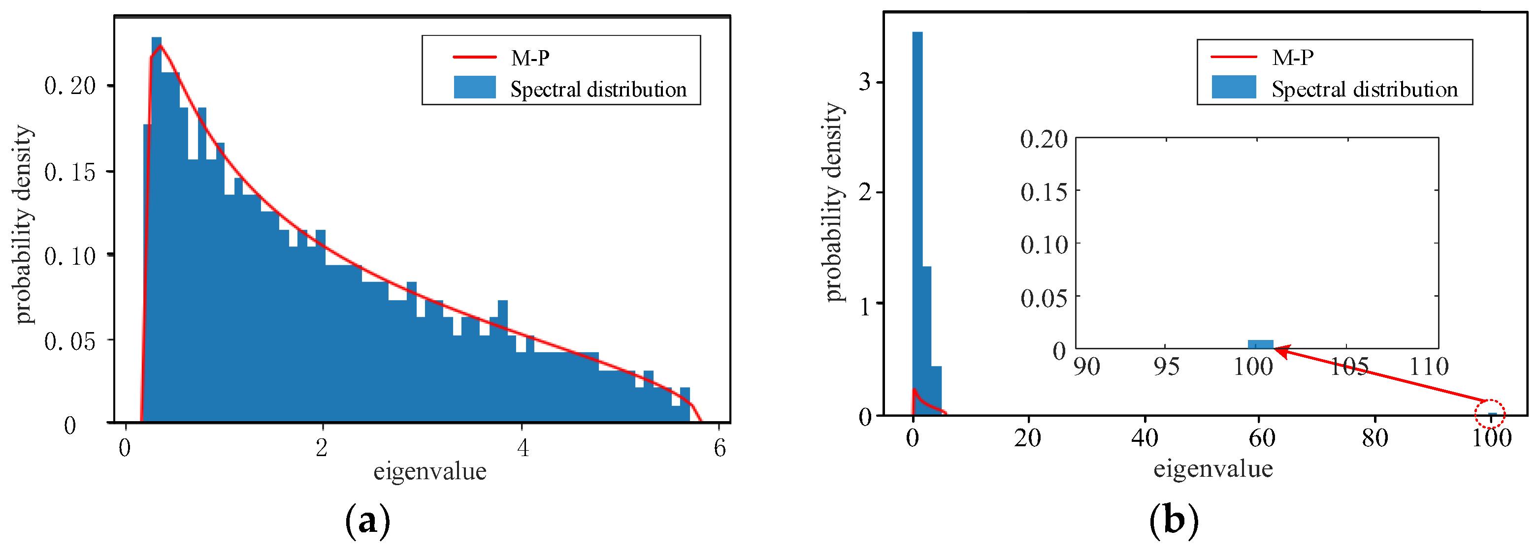
2.1.1. M-P Law

Let a random matrix ${\mathit{X}}_{N\times M}$ be a non-Hermitian matrix, where the elements are independently and identically distributed. The mean of the elements of the matrix is 0, and the variance is 1. Then we can obtain the corresponding covariance matrix S as follows:

$$\mathit{S}=\frac{1}{N}\mathit{X}{\mathit{X}}^H$$

(1)

where H denotes taking the conjugate transpose.

Let p = N/M, which requires 0 < p ≤ 1 in practical applications. According to random matrix theory, when M, N→∞, the empirical spectrum distribution function of the covariance matrix S converges non-randomly to the probability density function. The probability density function is as follows:

$$f\left({\lambda }_{\mathit{S}}\right)=\left\{\begin{array}{l}\frac{1}{2\pi p{\sigma }^{2}x}\sqrt{(b-x)(x-a)},\hspace{1em}a⩽x⩽b\hfill \\ 0\hspace{1em}\hspace{1em}\hspace{1em}\hspace{1em}\hspace{1em}\hspace{1em}\hspace{1em}\hspace{1em},\hspace{1em}\hspace{1em}\mathrm{others}\hfill \end{array}\right.$$

(2)

where ${\lambda }_{\mathit{S}}$ represents the eigenvalue of the covariance matrix S. $a={\sigma }^2{(1-\sqrt{p})}^2$, $b={\sigma }^2{(1+\sqrt{p})}^2$, a and b represent the upper and lower bounds of the eigenvalues, respectively. σ² is the variance of all elements in the random matrix ${\mathit{X}}_{N\times M}$.

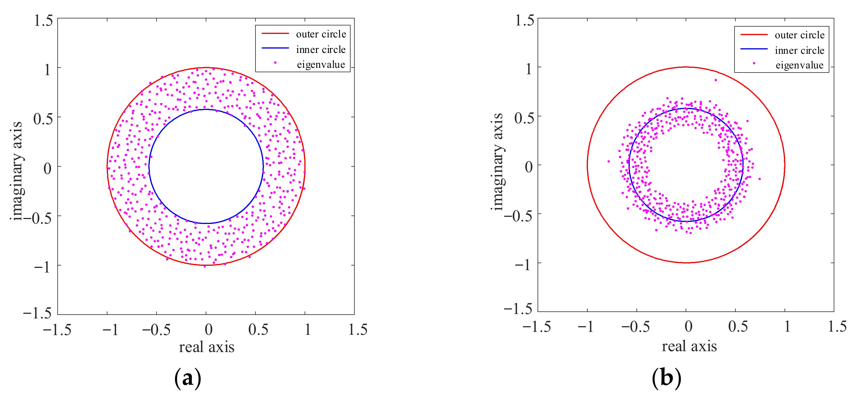
2.1.2. Ring Law

Assume that there are a number of standard independent non-Hermitian matrices of matrix ${\mathit{X}}_i$(i = 1, 2, 3, …, l), ${\mathit{X}}_i\in C^{N\times M}$. In order to map the matrix to the complex plane, each matrix is transformed as follows:

$${\mathit{X}}_{u,i}=\mathit{U}\sqrt{{\mathit{X}}_i{\mathit{X}}_i{}^H}$$

(3)

where ${\mathit{X}}_{u,i}$ is the singular value equivalence matrix of X_i. U is a Haar distributed unitary matrix.

Let $\mathit{W}={\displaystyle \prod _{i=1}^L{\mathit{X}}_{u,i}}$, then the standard matrix product $\widehat{\mathit{W}}$ is obtained by normalizing W according to Equation (4).

$${\widehat{w}}_i=\frac{w_i}{\sqrt{M}\sigma (w_i)}$$

(4)

where ${\widehat{w}}_i$, $w_i$ denote the row vectors of row i in matrices $\widehat{\mathit{W}}$ and W, respectively, and $\sigma (w_i)$ is the standard deviation of $w_i$.

According to random matrix theory, when M, T→∞, the empirical spectral density of the $\widehat{\mathit{W}}$ will converge in the circle of the probability density functions on the complex plane. The probability density function is given by:

$$f({\lambda }_{\widehat{w}})=\left\{\begin{array}{cc}\frac{1}{\pi pL}|{\lambda }_{\widehat{w}}{|}^{\frac{2}{L-2}},& {(1-p)}^{\frac{L}{2}}\le \left|{\lambda }_{\widehat{w}}\right|\le 1\\ 0,& \mathrm{others} \end{array}\right.$$

(5)

where p = N/M, and p ∈ [0, 1]. ${\lambda }_{\widehat{w}}$ is the eigenvalue of $\widehat{\mathit{W}}$. The inner ring of the circle has a radius of ${(1-p)}^{L/2}$, and the outer ring has a radius of 1.

2.2. Grid Matrix Model

The actual grid is a system with a highly complex topology. In order to sense the current state of the grid, measurement devices are usually deployed in the system. In this paper, we assume that each node in the system is equipped with a measurement device.

Suppose there is a power system with N nodes, where each node has k volumes to measure at a given time. Then the system has M = N × k state volume data in total. The system at the moment can be represented by a vector x(t) as follows:

$$x(t)=\left[x_1(t),x_2(t),x_3(t)\hspace{1em},\cdots ,x_M(t)\right]$$

(6)

As the sampling time increases continuously, a two-dimensional matrix X describing the state of the system is formed:

$$\mathit{X}=\left[\begin{array}{cccccc}{x}_1(t_1),& x_1(t_2),& x_1(t_3),& \cdots ,& x_1(t_n),& \cdots \\ x_2(t_1),& x_2(t_2),& x_2(t_3),& \cdots ,& x_2(t_n),& \cdots \\ x_3(t_1),& x_3(t_2),& x_3(t_3),& \cdots ,& x_3(t_n),& \cdots \\ ⋮& ⋮& ⋮& & ⋮& \\ x_M(t_1),& x_M(t_2),& x_M(t_3),& \cdots ,& x_M(t_n),& \cdots \end{array}\right]$$

(7)

Intercepting X in a time window of width T forms an M × T system state matrix ${\mathit{X}}_{M\times T}$, which contains both system state data at the current t_n moment and historical data for the previous T−1 lengths:

$${\mathit{X}}_{M\times T}=\left[\begin{array}{cccc}{x}_1(t_{n-T+1}),& x_1(t_{n-T+2}),& \cdots & x_1(t_n)\\ x_2(t_{n-T+1}),& x_2(t_{n-T+2}),& \cdots & x_2(t_n)\\ x_3(t_{n-T+1}),& x_3(t_{n-T+2}),& \cdots & x_3(t_n)\\ ⋮& ⋮& & ⋮\\ x_M(t_{n-T+1}),& x_M(t_{n-T+2}),& \cdots & x_M(t_n)\end{array}\right]$$

(8)

The data in ${\mathit{X}}_{M\times T}$ is constantly updated as the grid operation time is updated, so that the real-time state of the grid can be monitored in time. Meanwhile, in order to eliminate the effects of different orders of magnitudes, it is necessary to normalize the matrix. The standardized matrix $\widehat{\mathit{X}}$ is a standard non-Hermitian matrix, where each row satisfies a mean of 0 and a standard deviation of 1. The row vectors of ${\mathit{X}}_{M\times T}$ are normalized as follows:

$$\begin{array}{c}{\widehat{x}}_{i,j}=\left(x_{i,j}-{\overline{x}}_i\right)\times \left(\sigma \left({\widehat{x}}_i\right)/\sigma \left(x_i\right)\right)+{\overline{\widehat{x}}}_i\\ 1\le i\le M,\hspace{1em}\hspace{1em}\hspace{1em}\hspace{1em}1\le j\le \mathrm{T}\end{array}$$

(9)

where ${\widehat{x}}_{i,j}$, $x_{i,j}$ are the elements in row i and column j of $\widehat{\mathit{X}}$ and ${\mathit{X}}_{N\times M}$, respectively. ${\overline{x}}_i$ and $\sigma \left(x_i\right)$ represent the mean and standard deviation of row i in ${\mathit{X}}_{N\times M}$, respectively. ${\overline{\widehat{x}}}_i$ and $\sigma \left({\widehat{x}}_i\right)$ represent the mean and standard deviation of row i of $\widehat{\mathit{X}}$, respectively. ${\overline{\widehat{x}}}_i=0$; $\sigma \left({\widehat{x}}_i\right)=1$.

Assume that a certain power system is known, and make its load proportionally increasing. As the power system operates, the state data at each node are collected. Then the original data state matrix of the system is formed according to the method presented in this paper. Then the raw data state matrix is pre-processed. The sliding window technique is used to intercept the pre-processed matrix; the sample matrices in different states can be obtained separately. The random matrix theory is used to analyze the sample matrix of the power grid in two different states, and the visualization results are shown in Figure 1 and Figure 2.

As shown in Figure 1 and Figure 2, the difference between the system in the normal and abnormal states can be clearly found. When the grid is operating steadily, the sample covariance random matrix of the system obeys the M-P law. The distribution of the eigenvalue spectrum of this matrix converges to the M-P law curve. Also, the singular value matrix of the sample matrix of the system obeys the ring law. The eigenvalues of the singular value matrix are distributed in the circular ring in the complex plane. However, when the load increases until the stable operation of the system is destroyed, the sample covariance random matrix of the system no longer obeys the M-P law, and isolated and large eigenvalues appear. Meanwhile, the eigenvalue distribution of the corresponding $\widehat{\mathit{W}}$ of the system will no longer obey the ring law; the eigenvalues of $\widehat{\mathit{W}}$ will cross the inner circle. It can be seen that these two laws of random matrix theory are good for detecting anomalies in the stable operation of the system.

2.3. Statistical Evaluation Metrics

According to the analysis in Section 2.2, the difference between the normal and abnormal grid operation can be easily reflected by random matrix theory. To quantify the nature of the grid when it deviates from a stable operation, it is necessary to define reasonable evaluation indicators by selecting appropriate statistics according to the two laws mentioned above.

2.3.1. Maximum Eigenvalue of Sample Covariance Matrix

According to the M-P law: When the system is abnormal, the law in stable operation is broken, and the eigenvalues of S no longer converge to f(λ_s), where the largest eigenvalue will exceed the boundary of the normal eigenvalue.

Let the maximum eigenvalue of S be ${\lambda }_{s(\max )}$. In the normal state, ${\lambda }_{s(\max )}\le {\lambda }_{s\left(lim\right)}$(where ${\lambda }_{s\left(lim\right)}={\sigma }^2{(1+\sqrt{p})}^2$. In abnormal state, ${\lambda }_{s\left(max\right)}>{\lambda }_{s\left(lim\right)}$. So, an indicator Δλ can be defined to describe the difference between the normal and abnormal states, and the indicator Δλ is given by:

$$\Delta \lambda ={\lambda }_{s(\max )}-{\lambda }_{s(\lim )}$$

(10)

when Δλ > 0, it means that there is an abnormality in the system; otherwise it means that the system is stable.

2.3.2. Mean Spectral Radius

Let the radius of the eigenvalues of the standard matrix product $\widehat{\mathit{W}}$ be λ_i (i = 1, 2, 3, …, M) and the radius of the inner loop of the ring law be R_inner. The mean spectral radius R_msr is a linear eigenvalue statistic that can be used to describe the overall distribution of eigenvalues. R_msr is given by:

$$R_{\mathrm{msr}}=\frac{1}{M}{\displaystyle \sum _{i=1}^M{\lambda }_i}$$

(11)

When the state of the physical system changes, the elements in the matrix change, causing R_msr to change accordingly. When R_msr > R_inner, it means that most of the eigenvalues are distributed inside the circle; then the system is stable. If the value of R_msr is larger than the value of R_inner, the more stable the system is; conversely, the system is unstable. The indicator d is proposed to determine whether the eigenvalues are distributed within the circle as follows:

$$d=R_{\mathrm{msr}}-R_{\mathrm{inner}}$$

(12)

when d > 0, it means that there is an abnormality in the system; otherwise it means that the system state is stable.

2.4. Discussion of Indicator Δλ and Indicator d

According to the above analysis, it can be seen that both index Δλ and index d can distinguish the normal operation state and abnormal operation state of the power grid. Therefore, both indicators can be used to evaluate the grid operation state. However, the roles of the two are different. The Δλ reflects the deviation of the maximum eigenvalue of the corresponding covariance matrix of the system, which is more prominent in terms of variance. The d reflects the overall average of the eigenvalues of the standard matrix product of the system’s random matrix, highlighting the overall nature more. Therefore, the trend analysis of index d can be considered as the basis for analyzing the trend of power grid stability.

3. Qualitative Trend Analysis

In this section, the qualitative trend analysis technique is introduced. It is a data-driven, semi-quantitative analysis technique that has been successfully applied to process monitoring and fault diagnosis field [27,33,34]. The general idea of qualitative trend analysis is to extract qualitative information from quantitative process data and to represent it in a symbolic language [27,28]. And the process of qualitative trend analysis consists of two stages: (1) trend extraction and (2) trend identification.

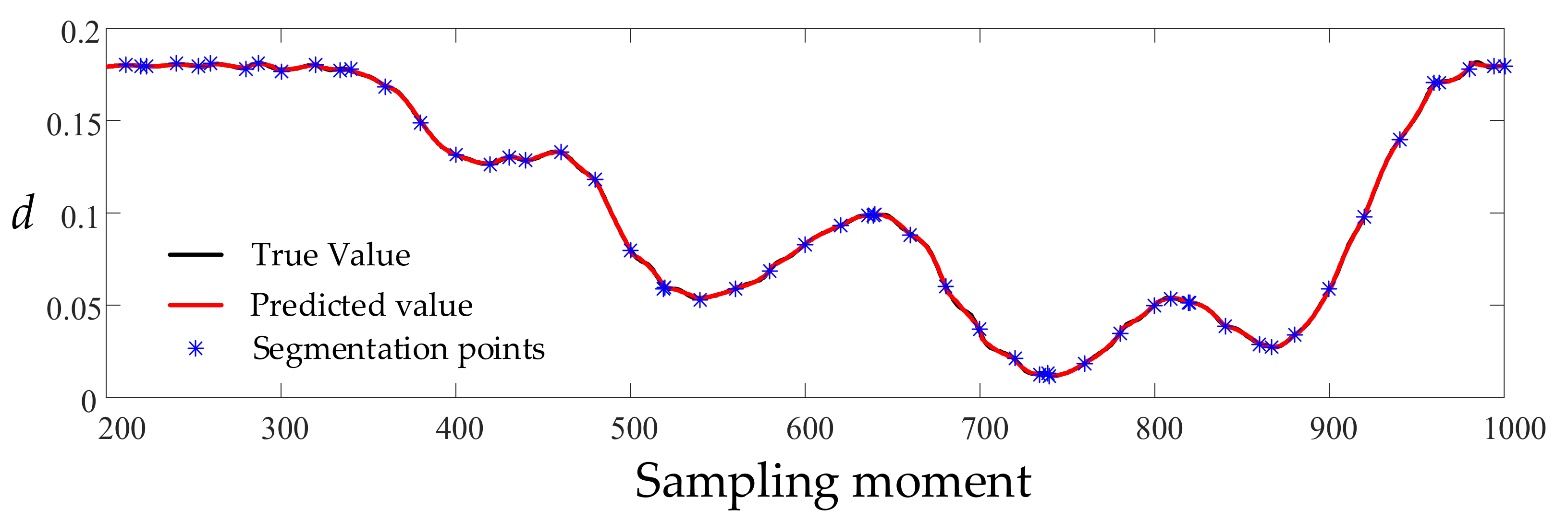
3.1. Trend Extraction

The trend extraction process is to split the target curve into some data segments, then to fit each data segment with a function separately and, finally, to extract the trend of that segment according to the fitting function.

In order to obtain better results for trend extraction, it is necessary to ensure sufficient accuracy and fast enough computation speed. In addition, it is also considered that the length of the data segment has an impact on the fitting effect. Therefore, in this paper, the trend extraction is performed by combining the F-test based on the time-sliding window technique, and the fitting function uses a quadratic polynomial. It is worth noting that the size of the time window used in this paper is variable, and its length is changed adaptively according to the fitting effect. This way, the data segment’s optimal segmentation result can be obtained.

Suppose there is a time series data D(t), and the starting moment is noted as t₀. The trend extraction process for D(t) is as follows.

(1)

Set the length of the initial time sliding window to L, and feed the values of the first L data into the time sliding window in turn.

(2)

Using a binomial function to fit the data in the time window, the obtained binomial fit function takes the form of the following equation:

$$f(t)=A{\left(t-t_0\right)}^2+B\left(t-t_0\right)+C$$

(13)

where A, B and C are the coefficients of the binomial function. The values of these three parameters are determined according to the ordinary least squares. The specific process is to minimize the sum of squares of the error between the fitted curve and the actual curve to find the best fitting function parameter combination of the data.

(3)

In order to judge the fitting effect of the data in the time sliding window, it is necessary to test the significance of the fitted model using the F-test. If the fitting effect meets the requirements, the window is expanded to include the data at the moment of $t_{L+1}$, refitted and the F-test is performed again until the F-test no longer meets the requirements. If the fitting effect does not meet the requirements, the fitting is re-fitted by reducing the window until it just meets the requirements of the F-test.

(4)

Check whether the fitted model in the window contains extreme value points in the interval. If so, split the data segment in two at that point, refit the two data segments separately and then perform the F-test.

(5)

After the previous data segment is determined by steps (3) and (4), a new time sliding window is used to fit the remaining data. To ensure that the data segments are continuous, the start moment of the current time sliding window should be the end moment of the previous data segment. Let the length of the time window remain the initial length. Then repeat steps (2), (3) and (4) to determine the new data segment. When the final number of remaining data is less than L, the remaining data are fitted directly.

(6)

Calculate the first-order derivatives and second-order derivatives of all extracted data segments in the interval to which they belong, respectively, and determine the signs of the first-order derivatives and second-order derivatives.

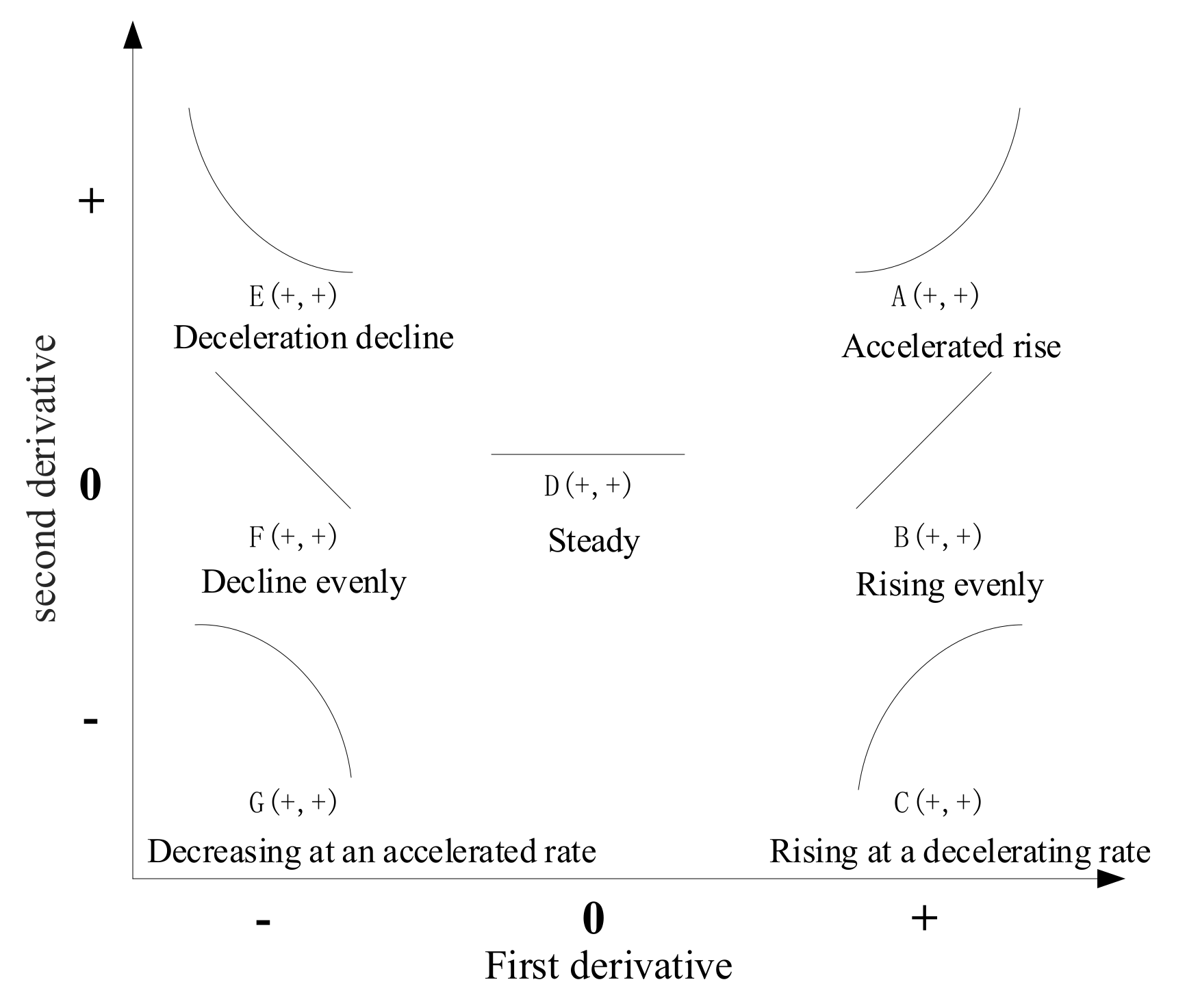
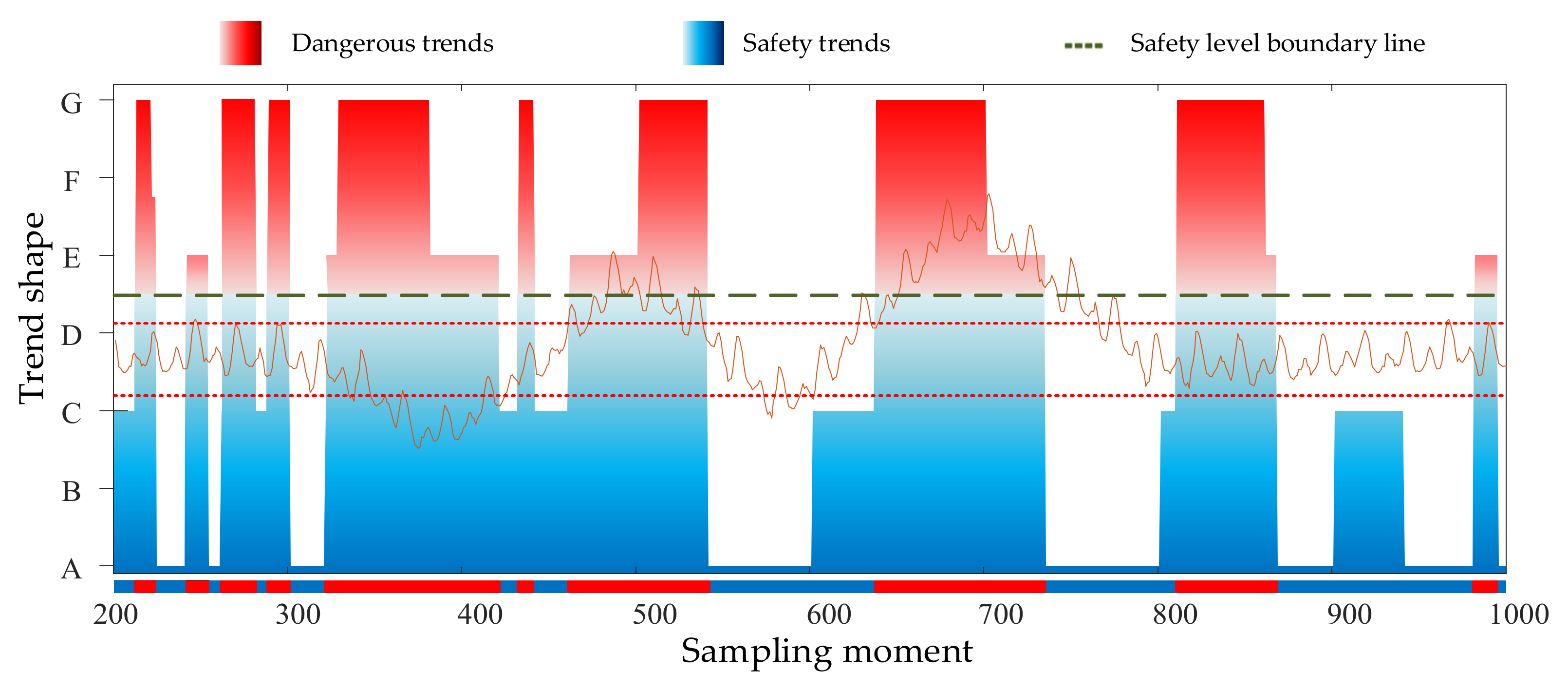
3.2. Trend Identification

Trend identification is to match the results of trend extraction with trend primitives, each of which can be described by a tuple consisting of the first-order derivative and second-order derivative symbols of the fitted model [35], as shown in Figure 3, where seven different trend primitives reflect seven different patterns of variation.

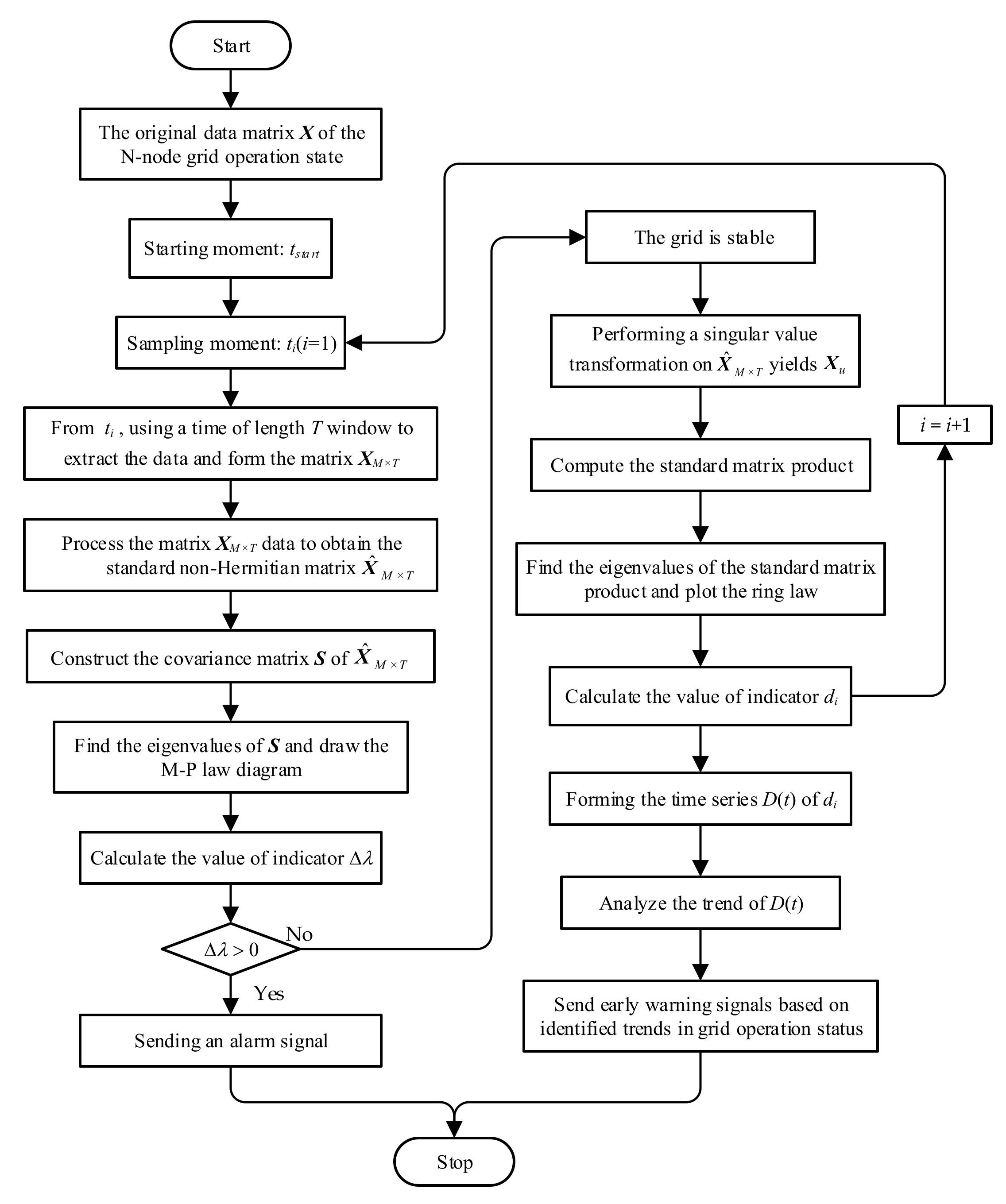
4. Process of Real-Time Grid Operation State Assessment

The grid operation condition evaluation in this paper focuses on the two causes of grid operation that lead to faults mentioned above. Combined with the analysis in Section 2 of this paper, indicator Δλ is more sensitive to the variability of the system, and indicator d reflects the overall performance of the system. Based on the characteristics of these two indicators, this paper proposes an evaluation method that can evaluate both whether the current operating state of the grid is normal and whether there is a bad trend in the normal operating state.

Suppose there is an N-node grid with k state variables at each node; then the specific process is shown in Figure 4.

To make it easier to judge the operating trend, the security trend level can be defined according to the trend shape, as shown in

Table 1. The table of safety level.

Primitives of the Trend	Trend Security Levels
A(+,+)	Safe
B(+,0)
C(+,−)
D(0,0)
E(−,+)	Dangerous
F(−,0)
G(−,−)

.

5. Experiment and Discussion

In order to verify that the proposed method is able to evaluate the current grid operation state for abnormalities as well as to detect the bad operation trends during normal grid operation, this paper designs simulations based on the IEEE 118-bus system. The simulations consist of two cases, one of which is a short-circuit fault in the grid and the other which is an abnormal load change in the stable operating range of the grid.

5.1. Example 1: Case of Short Circuit Fault Calculation

In this example, the state matrix of the grid (M = 118) is constructed with the voltage magnitude data of 118 nodes in the whole network. The data sampling step is set to 0.02 s, and a total of 1000 times are sampled, in which the grid operates normally from t₁ to t₄₀₀, and a short-circuit fault is set to occur at node 29 at t₄₀₁, which continues until the fault is cleared at t₅₀₀. Then the grid resumes stable operation. In order to simulate the error in the real sampling process, add Gaussian white noise of suitable size on the basis of the simulation data. The changes of the voltage of the whole network nodes during the whole process are shown in Figure 5.

Sample data are extracted with a time sliding window of length T (T = 200), which is then used to reconstruct a sample random matrix of system states for analysis. After analysis, the M-P law diagrams of the system in stable operation and in case of failure are obtained, respectively, as shown in Figure 6.

Figure 6 shows that after a short-circuit fault occurs, the system state changes and the state random matrix no longer obeys the M-P law. There are isolated eigenvalues with large values. Correspondingly, the Δλ > 0. During the simulation, the variation of the state assessment indicator Δλ of the grid is shown in Figure 7.

The value of the length of the time window is 200, and we need to wait for 200 sampling moments to enter the time window before we can get the state random matrix of the system. Therefore, the starting moment of a should be t₂₀₀ of the actual sampling moment because Δλ will return to the value at the normal operation of the grid only when the historical data of the system random matrix no longer contains the data of the abnormal state. Then the stop moment of the fault should be $t_{700-T}$.

Similarly, we can obtain the results of the analysis of the ring law and the variation curve of the indicator d. The results are shown in Figure 8 and Figure 9.

From the above results, it is clear that both Δλ and d can accurately assess whether a fault has occurred in the current grid during grid operation. Then, comparing the change curves of indicator Δλ and indicator d in Figure 6 and Figure 8, we can get the following information:

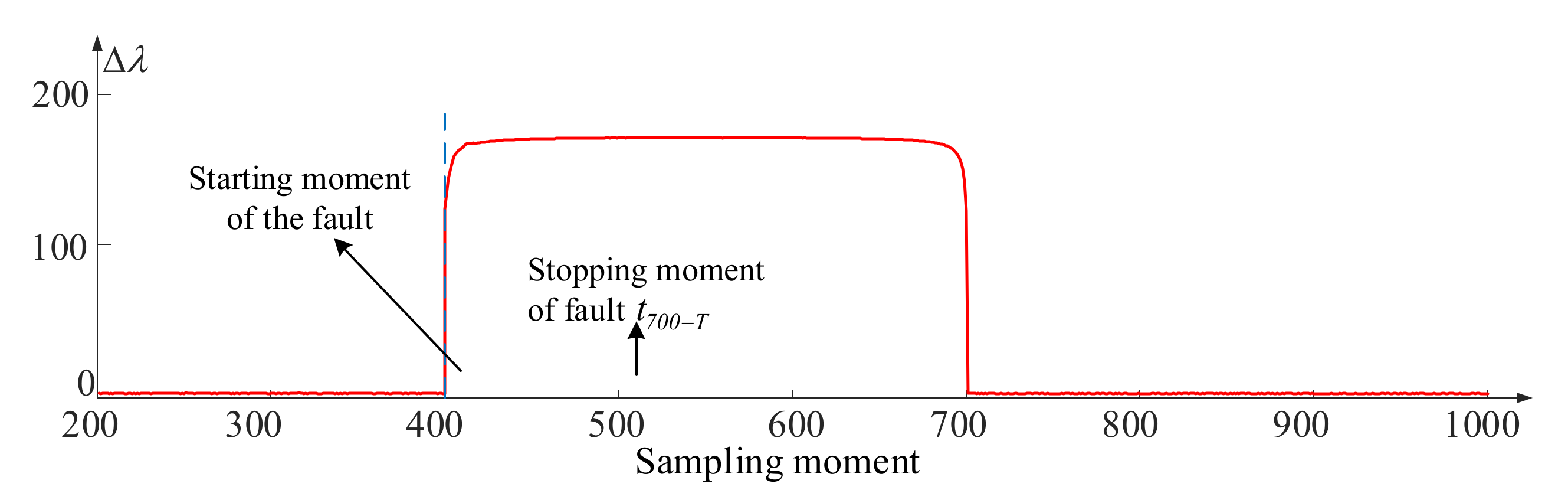
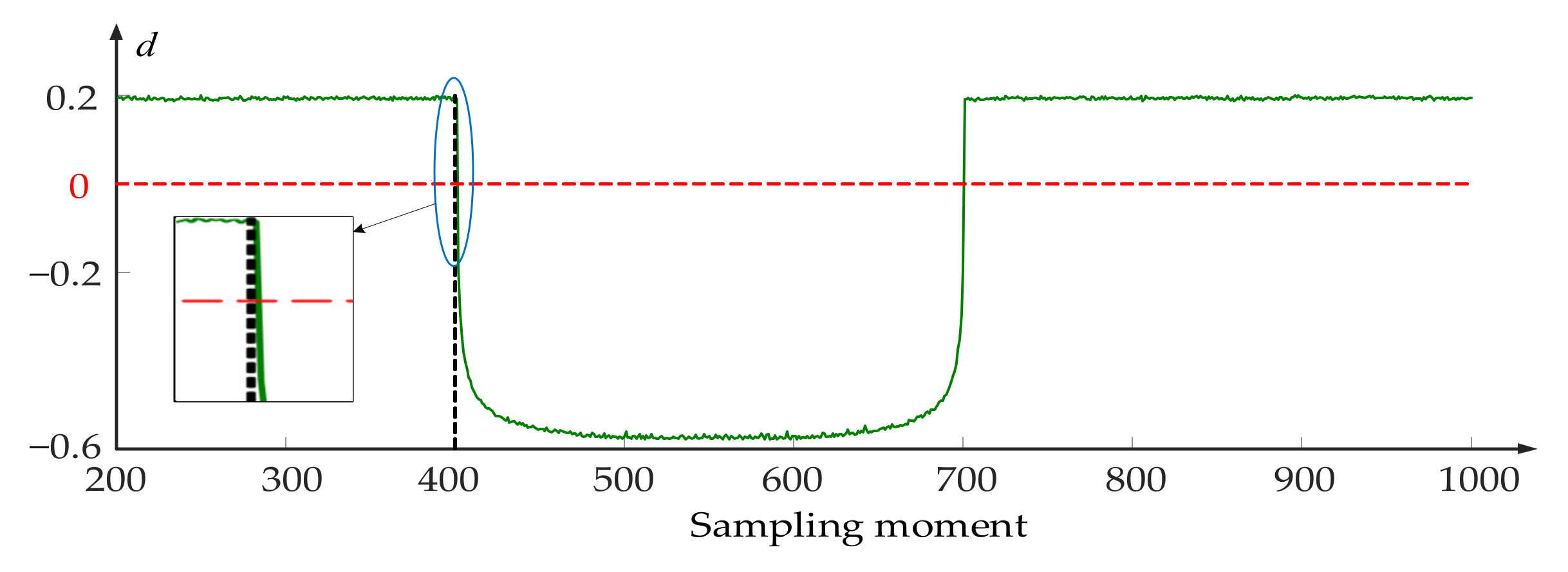
• In Figure 7, when the sampling moment is at t₄₀₁, the curve coincides with the line drawn at the moment t₄₀₁, while in Figure 8 the curve deviates from the drawn line. This indicates that the value of Δλ changes immediately after the system fault occurs, while the indicator d does not. It means that Δλ is more sensitive to capture the abnormal system state.
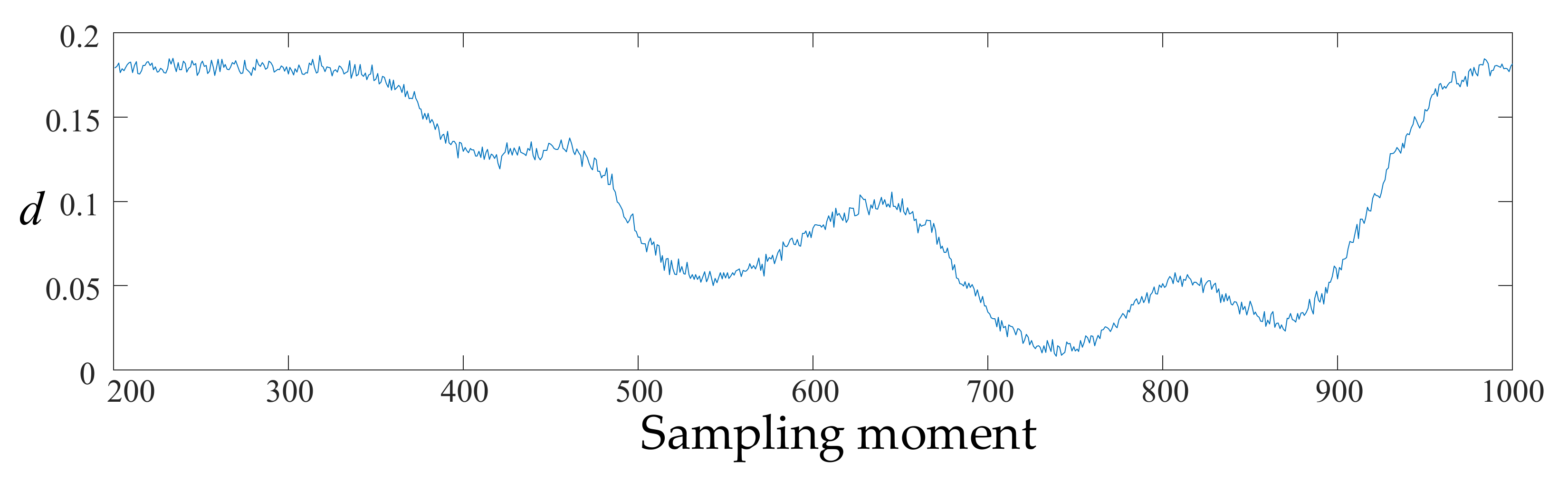
• In Figure 9, the curve of d is still greater than 0 for a short period of time after the fault, which indicates that the value of indicator d does not change to a value less than 0 immediately after the fault. It changes slowly. Thus, the operating state of the grid is still normal for a short period of time after the fault occurs, and the abnormal state of the grid can be detected only after a short period of time.

Therefore, the above results verify that Δλ is more sensitive to the perception of anomalous states than d, which is more suitable to reflect the holistic level of the system.

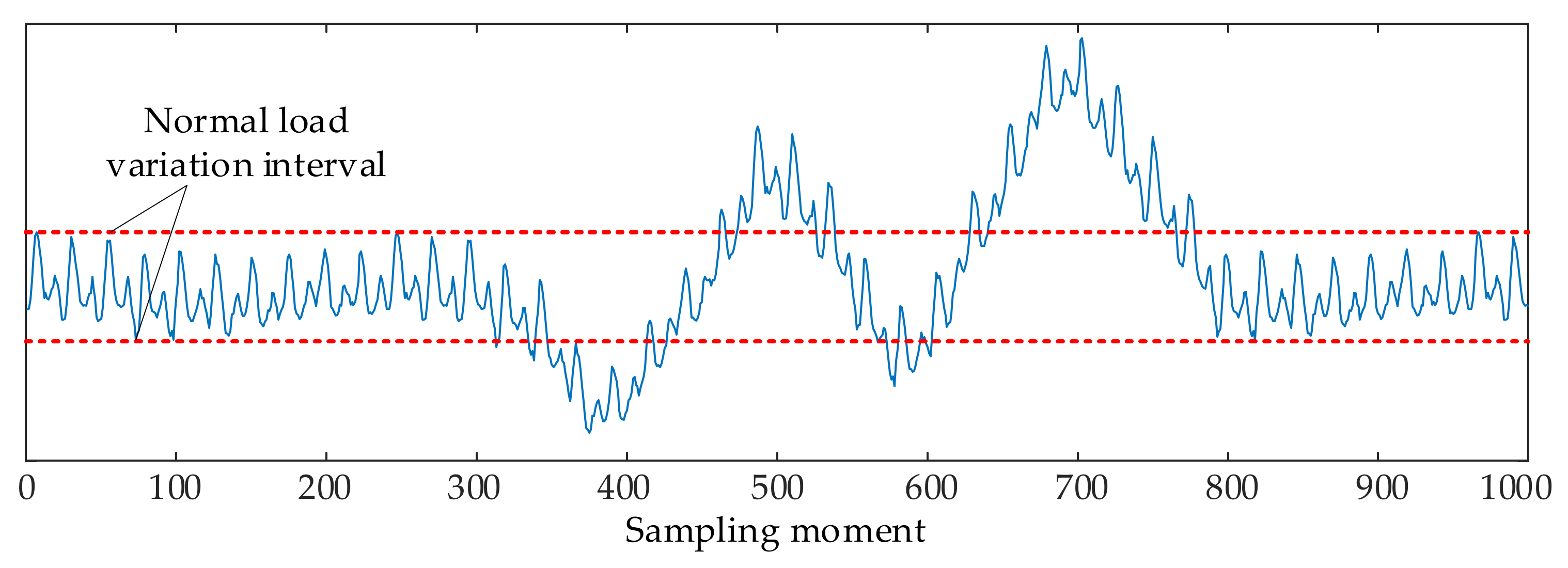
5.2. Example 2: Case of Abnormal Load Changes in the Stable Operating Range

In this case, the load at each node is varied in the range of normal and stable operation of the system, and the grid state matrix is still constructed with the voltage magnitude data of each node of the system.

The load is changed in the manner of Figure 10. A total of 1000 sampling points are set in the simulation process. The system keeps normal stable operation before t₃₀₀. From t₃₀₁, the load gradually deviates from the normal operation interval and continues until t₈₀₀. From t₈₀₁, the disturbance is cleared, and the system resumes stable operation. The length of the time window for intercepting data is set to 200. Then the state matrix obtained from each time window interception is analyzed and calculated in turn.

During the simulation, the values of Δλ and d have been in the interval of stable operation, which indicates that the system state has been stable. Then the change of d value is used to reflect the change of system operation state, as shown in Figure 11.

Since the value of T is 200, the start moment of d is t₂₀₀. The fluctuations of the curve in Figure 11 are due to errors caused by the data processing and the statistical characteristics of the random matrix. In order to reduce the noise interference and the influence of random matrix on the data, this paper uses wavelet transform to filter the curve of d. Then the curve of d was fitted according to the method in Section 3.1, and the initial value of L was set to 40. Then the adaptive segmentation points of the curve were obtained. The final results are shown in Figure 12, and the MSE error of the fitting results is 1.94 × 10⁻⁶.

When the data in the matrix remain stable, the value of d also remains broadly stable; when the stability law of the data in a dimension of the matrix is broken, the value of d decreases, and the greater the difference from the original data change law, the more the value of d decreases. From Figure 12, it can be seen that the system operates stably in the normal interval before moment t₃₀₀, and since moment t₃₀₁, the system is disturbed and the load deviates from the normal interval, which makes the data in the normal interval in the matrix decrease, and the value of d decreases as a result. When the load value changes again close to the normal interval, the value of d will increase slightly. It can be seen that the change of d reflects the change of grid operation state. Therefore, the trend of d is the trend of the operating state of the grid. Thus, the trend extraction results of d are shown in

Table 2. Trend extraction results table.

Data Segment Number	Time Interval	Trend Shape	Data Segment Number	Time Interval	Trend Shape
1	(200, 211)	C	27	(600, 620)	C
2	(211, 220)	G	28	(620, 636)	C
3	(220, 223)	E	29	(636, 640)	G
4	(223, 240)	A	30	(640, 660)	G
5	(240, 253)	E	31	(660, 680)	G
6	(253, 260)	A	32	(680, 700)	G
7	(260, 280)	G	33	(700, 720)	E
8	(280, 287)	C	34	(720, 734)	E
9	(287, 300)	G	35	(734, 740)	A
10	(300, 320)	A	36	(740, 760)	A
11	(320, 334)	E	37	(760, 780)	A
12	(334, 340)	A	38	(780, 800)	A
13	(340, 360)	G	39	(800, 809)	C
14	(360, 380)	G	40	(809, 820)	G
15	(380, 400)	E	41	(820, 840)	G
16	(400, 420)	E	42	(840, 860)	G
17	(420, 431)	C	43	(860, 867)	E
18	(431, 440)	G	44	(867, 880)	A
19	(440, 460)	C	45	(880, 900)	A
20	(460, 480)	E	46	(900, 920)	C
21	(480, 500)	E	47	(920, 940)	C
22	(500, 520)	G	48	(940, 960)	A
23	(520, 540)	G	49	(960, 963)	E
24	(540, 560)	A	50	(963, 980)	A
25	(560, 580)	A	51	(980, 994)	E
26	(580, 600)	A	52	(994, 1000)	A

.

As shown in Table 2, the trend shape changes with the operation of the grid. In Table 2, some of the trend shapes have a short duration (e.g., data segments with serial numbers 3, 6 and 8). The change of d in these time periods is not obvious, so it can be considered as the fluctuation that occurs when the system is operating normally and belongs to the data segment that has little effect on the value of d. Therefore, the trend behavior of this part can be ignored in the analysis. What is really worth attention is the data segment with a long duration of the dangerous trend level. The longer the duration of the dangerous trend, the more the system deviates from the normal operation interval, which indicates that there may be some hidden danger in the system, causing the stable operation state of the system to deteriorate. In order to present the changes of the safety trend more visually, it can be plotted as the safety trend distribution shown in Figure 13.

The safety level is defined for each trend segment according to Table 1, and the trend shapes of different safety levels are distinguished by color. As shown in Figure 13, the top of the safety level divider is the danger trend (red area), and the bottom is the safety trend (blue area). Also, red and blue colored progress bars are set at the bottom of the graph for tracking the duration of the safety and hazard trends. Because there are fluctuations in the system with a short duration of the trend shape, the dangerous trend time set must have a lower limit in order to avoid the small trend segments in the system that do not affect the d. Considering the error and margin, Example 2 sets this lower limit value of duration to 60. It means that the part of the dangerous trend duration exceeding 60 moments is considered as a bad trend where the load does exist. From Figure 12 it can be found that there are four dangerous trend segments that last for a longer period of time. By comparing with the load variation curve, it is found that the first three long dangerous trend segments correspond to the part of the load when it is outside the normal interval, so it can be seen that the abnormal load variation can be captured more accurately by analyzing the trend of d. At the fourth dangerous trend segment, it is found that the load has returned to within the normal interval but still shows a dangerous trend, which is due to the fact that the random matrix still contains a large amount of historical data with load perturbations when the data within the random matrix has just reached the t₈₀₀ moment. Therefore, it can be considered that, whenever there is a long period of dangerous trend segments, there is a bad operating trend indicated in the current system.

In summary, Example 1 compares two state assessment indicators Δλ and d. Through analysis, it is found that indicator Δλ is more sensitive to the abnormal state of the grid and is more suitable as a basis for assessing the abnormal behavior of the grid, while indicator d focuses on the overall state of the grid and is therefore more suitable as a trend assessment indicator. The results of Example 1 verify the discussion in Section 2.4 of this paper. Example 2 is focused on whether there is a bad operating trend of the grid under normal conditions. Based on the assessment of the stability of the grid operation by using indicator Δλ, further simulation experiments verify that the trend of d can reflect the operating trend of the grid well, and the analysis of the trend of d by using the qualitative trend analysis technique can effectively find the unstable operating trend during operation.

6. Conclusions

The causes of faults during grid operation can be broadly divided into two types: one is sudden faults, and the other is deterioration of poor operating conditions. To address this issue, this paper proposes an evaluation method that can determine both whether the current state of the power grid is stable and whether there is a bad operating trend in the current power grid. Firstly, two indicators are defined separately by random matrix theory: Δλ and d. By comparison, it is found that the former can sensitively determine whether the system is stable or not, and the latter, combined with qualitative trend analysis technique, can effectively discover the undesirable trends in the grid operation process. Thus, the method in this paper uses both indicators to evaluate simultaneously, and if Δλ is greater than 0, it means that the current grid is unstable and an alarm signal should be issued. If Δλ is less than 0, a trend analysis is performed on d. If the decomposition results determine that the current d is in a dangerous trend segment and the duration of the danger exceeds a given value, then an alert signal is issued. If Δλ is less than 0 and there is no dangerous trend segment for d, then it means that the current state of the grid is stable. The feasibility of the method proposed in this paper is verified by the simulations of two examples.

Compared with the traditional analysis method, the method proposed in this paper ignores the complex physical structure of the power grid and uses the data generated during the operation of the power grid more effectively, which provides a new research idea for understanding the operation law of the power grid. The simulation results show that the method cannot only accurately evaluate the current operating state of the power grid but can also find the bad trend in the operation of the power grid. It is worth noting that the work in this paper is mainly to evaluate the current state and trend of the power grid. It is not yet possible to locate the location of the anomaly, so the subsequent research can continue to focus on fault location and fault cause analysis.

References

- US Department of Energy. The Smart Grid. 2021. Available online: https://www.smartgrid.gov/the_smart_grid/smart_grid.html (accessed on 20 July 2021).
- Hatziargyriou, N.; Milanovic, J.; Rahmann, C.; Ajjarapu, V.; Canizares, C.; Erlich, I.; Hill, D.; Hiskens, I.; Kamwa, I.; Pal, B.; et al. Definition and Classification of Power System Stability—Revisited & Extended. IEEE Trans. Power Syst. 2021, 36, 3271–3281. [Google Scholar] [CrossRef]
- Souxes, T.; Vournas, C. System stability issues involving distributed sources under adverse network conditions. In Proceedings of the 2017 IREP Symposium Bulk Power System Dynamics and Control—X (IREP), Espinho, Portugal, 28 August–1 September 2017; Volume 10, pp. 1–9. [Google Scholar]
- Wang, X.; Blaabjerg, F. Harmonic stability in power electronic based power systems: Concept, modeling, and analysis. IEEE Trans. Smart Grid 2019, 10, 2858–2870. [Google Scholar] [CrossRef] [Green Version]
- Mostafa, N.; Ramadan, H.S.M.; Elfarouk, O. Renewable energy management in smart grids by using big data analytics and machine learning. Mach. Learn. Appl. 2022, 9, 100363. [Google Scholar] [CrossRef]
- Syed, D.; Zainab, A.; Ghrayeb, A.; Refaat, S.; Abu-Rub, H.; Bouhali, O. Smart Grid Big Data Analytics: Survey of Technologies, Techniques, and Applications. IEEE Access 2021, 9, 59564–59585. [Google Scholar] [CrossRef]
- Hou, L.; Zhang, Y.; Yu, Y.; Shi, Y.; Liang, K. Overview of Data Mining and Visual Analytics towards Big Data in Smart Grid. In Proceedings of the 2016 International Conference on Identification, Information and Knowledge in the Internet of Things (IIKI), Beijing, China, 20–21 October 2016; pp. 453–456. [Google Scholar]
- Zainab, A.; Ghrayeb, A.; Syed, D.; Abu-Rub, H.; Refaat, S.S.; Bouhali, O. Big Data Management in Smart Grids: Technologies and Challenges. IEEE Access 2021, 99, 73046–73059. [Google Scholar] [CrossRef]
- Bhattarai, B.P.; Paudyal, S.; Luo, Y.; Mohanpurkar, M.; Cheung, K.; Tonkoski, R.; Hovsapian, R.; Myers, K.S.; Zhang, R.; Zhao, P.; et al. Big Data Analytics in Smart Grids: State-of-the-art, Challenges, Opportunities, and Future Directions. IET Smart Grid 2019, 2, 141–154. [Google Scholar] [CrossRef]
- Sayghe, A.; Hu, Y.; Zografopoulos, I.; Liu, X.; Dutta, R.G.; Jin, Y.; Konstantinou, C. Survey of machine learning methods for detecting false data injection attacks in power systems. IET Smart Grid 2020, 3, 581–595. [Google Scholar] [CrossRef]
- Ghorbanian, M.; Dolatabadi, S.H.; Siano, P. Big Data Issues in Smart Grids: A Survey. IEEE Syst. J. 2019, 13, 4158–4168. [Google Scholar] [CrossRef]
- Ma, L.; Zhang, X. Economic Operation Evaluation of Active Distribution Network Based on Fuzzy Borda Method. IEEE Access 2020, 8, 29508–29517. [Google Scholar] [CrossRef]
- Wang, T.; Du, Z.; Zhang, K.; Chen, K.; Xiao, F.; Ye, P. Reliability evaluation of high voltage direct current transmission protection system based on interval analytic hierarchy process and interval entropy method mixed weighting. Energy Rep. 2021, 7, 90–99. [Google Scholar] [CrossRef]
- Ma, J.; Liu, X. Evaluation of health status of low-voltage distribution network based on order relation-entropy weight method. Power Syst. Prot. Control 2017, 6, 87–93. [Google Scholar]
- Yang, J.; Liu, S.; Lu, Z.; Yan, Z.; Xu, X. Source-Grid-Load Combined Security Assessment of PV-Penetrated Distribution Network. In Proceedings of the 12th IEEE PES Asia-Pacific Power and Energy Engineering Conference (APPEEC), Nanjing, China, 20–23 September 2020; pp. 1–5. [Google Scholar]
- Liang, Y.-C.; Pan, G.; Bai, Z.D. Asymptotic Performance of MMSE Receivers for Large Systems Using Random Matrix Theory. IEEE Trans. Inf. Theory 2007, 53, 4173–4190. [Google Scholar] [CrossRef]
- Jalan, S.; Bandyopadhyay, J.N. Random matrix analysis of complex networks. Phys. Rev. E 2007, 76, 46107. [Google Scholar] [CrossRef] [Green Version]
- He, X.; Ai, Q.; Qiu, R.C.; Huang, W.; Piao, L.; Liu, H. A Big Data Architecture Design for Smart Grids Based on Random Matrix Theory. IEEE Trans. Smart Grid 2015, 8, 674–686. [Google Scholar] [CrossRef] [Green Version]
- Xu, X.; He, X.; Ai, Q.; Qiu, R.C. A Correlation Analysis Method for Power Systems Based on Random Matrix Theory. IEEE Trans. Smart Grid 2015, 8, 1811–1820. [Google Scholar] [CrossRef] [Green Version]
- He, X.; Chu, L.; Qiu, R.C.; Ai, Q.; Ling, Z.; Zhang, J. Invisible Units Detection and Estimation Based on Random Matrix Theory. IEEE Trans. Power Syst. 2019, 35, 1846–1855. [Google Scholar] [CrossRef] [Green Version]
- He, X.; Qiu, R.; Ai, Q.; Zhu, T. A Hybrid Framework for Topology Identification of Distribution Grid with Renewables Integration. IEEE Trans. Power Syst. 2021, 36, 1493–1503. [Google Scholar] [CrossRef]
- Zhang, Q.; Wan, S.; Wang, B.; Gao, D.W.; Ma, H. Anomaly detection based on random matrix theory for industrial power systems. J. Syst. Archit. 2019, 95, 67–74. [Google Scholar] [CrossRef]
- Xiong, Y.; Yao, W.; Chen, W.; Fang, J.; Ai, X.; Wen, J. A data-driven approach for fault time determination and fault area location using random matrix theory. Int. J. Electr. Power Energy Syst. 2020, 116, 105566. [Google Scholar] [CrossRef]
- Wu, Q.; Zhang, D.; Liu, D.W.; Liu, W.; Deng, C.Y. A method for power system steady stability situation assessment based on random matrix theory. Proc. CSEE 2016, 36, 5414–5420. [Google Scholar]
- Liu, W.; Zhang, D.; Wang, X.; Liu, D.; Wu, Q. Power system transient stability analysis based on random matrix theory. Proc. CSEE 2016, 36, 4854–4863. [Google Scholar]
- Thuerlimann, C.M.; Villez, K. Input estimation as a qualitative trend analysis problem. Comput. Chem. Eng. 2017, 107, 333–342. [Google Scholar] [CrossRef]
- Guo, Q.; Li, S.; Gong, Y.; Wang, F.; Yu, G. Application of qualitative trend analysis in fault diagnosis of entrained-flow coal-water slurry gasifier. Control Eng. Pract. 2021, 112, 104835. [Google Scholar] [CrossRef]
- Li, Y.; Cao, W.; Gopaluni, R.B.; Hu, W.; Cao, L.; Wu, M. False alarm reduction in drilling process monitoring using virtual sample generation and qualitative trend analysis. Control Eng. Pract. 2023, 133, 105457. [Google Scholar] [CrossRef]
- Da Silva, P.R.N.; Gabbar, H.A.; Junior, P.V.; Junior, C.T.D.C. A new methodology for multiple incipient fault diagnosis in transmission lines using QTA and Naïve Bayes classifier. Int. J. Electr. Power Energy Syst. 2018, 103, 326–346. [Google Scholar] [CrossRef]
- García, A. Global financial indices and twitter sentiment: A random matrix theory approach. Phys. A Stat. Mech. Its Appl. 2016, 461, 509–522. [Google Scholar] [CrossRef]
- Palese, L.L. Random Matrix Theory in molecular dynamics analysis. Biophys. Chem. 2015, 196, 1–9. [Google Scholar] [CrossRef]
- Kato, R.; Yamanaka, M.; Kobayashi, M. Application of unfolding transformation in the random matrix theory to analyze in vivo neuronal spike firing during awake and anesthetized conditions. J. Pharmacol. Sci. 2018, 136, 172–176. [Google Scholar] [CrossRef]
- Gamero, F.I.; Meléndez, J.; Colomer, J. Process diagnosis based on qualitative trend similarities using a sequence matching algorithm. J. Process Control 2014, 24, 1412–1424. [Google Scholar] [CrossRef]
- Thuerlimann, C.M.; Duerrenmatt, D.J.; Villez, K. Soft-sensing with qualitative trend analysis for wastewater treatment plant control. Control Eng. Pract. 2018, 70, 121–133. [Google Scholar] [CrossRef]
- Araújo, A. Polynomial regression with reduced over-fitting—The PALS technique. Measurement 2018, 124, 515–521. [Google Scholar] [CrossRef]