Article

Liquified Petroleum Gas-Fuelled Vehicle CO2 Emission Modelling Based on Portable Emission Measurement System, On-Board Diagnostics Data, and Gradient-Boosting Machine Learning

by
Maksymilian Mądziel
Faculty of Mechanical Engineering and Aeronautics, Rzeszow University of Technology, 35-959 Rzeszow, Poland
Energies 2023, 16(6), 2754; https://doi.org/10.3390/en16062754
Submission received: 1 March 2023 / Revised: 11 March 2023 / Accepted: 13 March 2023 / Published: 15 March 2023
(This article belongs to the Section B: Energy and Environment)

Abstract

:
One method to reduce CO2 emissions from vehicle exhaust is the use of liquified petroleum gas (LPG) fuel. The global use of this fuel is high in European countries such as Poland, Romania, and Italy. There are a small number of computational models for the purpose of estimating the emissions of LPG vehicles. This work is one of the first to present a methodology for developing microscale CO2 emission models for LPG vehicles. The developed model is based on data from road tests using the portable emission measurement system (PEMS) and on-board diagnostic (OBDII) interface. This model was created from a previous exploratory data analysis while using gradient-boosting machine learning methods. Vehicle velocity and engine RPM were chosen as the explanatory variables for CO2 prediction. The validation of the model indicates its good precision, while its use is possible for the analysis of continuous CO2 emissions and the creation of emission maps for environmental analyses in urban areas. The validation coefficients for the selected gradient-boosting method of modelling CO2 emissions for an LPG vehicle are the R2 test of 0.61 and the MSE test of 0.77.

1. Introduction

Progressive climate change is forcing global authorities to continuously reduce anthropogenic greenhouse gas (GHG) production [1,2]. Global warming and climate change in relation to CO2 production, account for around 72% of global GHG production [3]. For the countries of the European Union, all sectors have already reduced their GHG production, except one [4,5]. This sector is transport, which accounts for 20% of global carbon dioxide (CO2) emissions [6]. The same values of CO2 emissions apply to the European Union, and politicians’ actions to reduce these emissions include, for example, shifting some road transport to rail [7,8]. Another way of counteracting this phenomenon is through the decision taken by the European Commission to introduce, among other things, a number of regulations on CO2 emissions from vehicles [9]. These include Regulations No. 443/2009 and 333/2014, which set a target of reducing the CO2 emission factor to 95 g/km for vehicles manufactured from 2020 onwards for the M1 segment [10,11]. To achieve the goal of reducing GHG emissions from transport by at least 60% by 2050 compared to 1990, the maximum CO2 emissions from vehicles for 2030 should be around 70 g/km [12,13]. Such targets and the associated demands on vehicle manufacturers are a major challenge that involves a number of design and technological changes to vehicles.
One way to reduce CO2 emissions is to use liquefied petroleum gas (LPG) to power vehicles [14,15]. It consists of hydrocarbons, as well as mixtures such as propane, butane, and isomers, liquefied under pressure and derived from oil or natural gas [16]. LPG is an odourless, colourless, and flammable gas that is heavier than air. Under normal conditions, LPG is in a gaseous state, but it is stored in special tanks and cylinders under pressure [17]. The most common vehicles running on LPG are bi-fuel vehicles, for which the supplementary fuel is LPG [18]. Solutions of this type are not popular worldwide; however, there are countries where the use of LPG fuel to power the vehicle is very popular. Countries that have a large fleet of LPG vehicles include the following: Turkey (4.7 million), Poland (3.1 million), Russia (3 million), Italy (2.4 million), India (2.4 million), Ukraine (2.3 million), and South Korea (2.1 million) [19,20]. The number of these vehicles in the countries mentioned is constantly increasing [21]. For example, in Poland, there are currently approximately 1550 companies that provide LPG installation services for vehicles [22]. However, there is also a group of vehicles produced by manufacturers that have a factory-installed LPG system, usually as an alternative fuel to petrol. The LPG fuel used in power vehicles has a high calorific value and reduced CO2 emissions compared to petrol vehicles [23]. Because propane and butane have a chemical structure of gasoline-forming hydrocarbons, they are lighter [24].
Consequently, there are two problems in modelling emissions from an LPG vehicle within the scope of the topic being pursued. The first is the low popularity of this fuel worldwide for the power of vehicles. This state of affairs results in a small database of data available from emissions tests for this type of vehicle. The existence of prediction models for this type of fuel is small compared to emission models for pure gasoline, diesel, and hybrid vehicles. The second issue is that there is a need for accurate emissions from vehicles running on LPG, especially in countries for which the use of this fuel is popular. The use of emission models currently available has some limitations. An example of a model that contains modelled emissions data for LPG bi-fuel vehicles is the COPERT software [25]. COPERT is an emissions model created by the European Environment Agency (EEA) and is widely used, among others, by national or local authorities, research institutes, and industry [26,27]. However, it is a model which allows for macroscale emission estimation, so in fact it is possible to derive emission results from it for its sum or for the emission factor parameter [28]. For the results obtained from emission models, the microscale is also an important aspect. At the microscale, for example, it is possible to determine the instantaneous emission of the vehicle on the selected part of the route [29]. Microscale models can also be used to determine an emission map, which makes it possible to observe locations where emissions from vehicles running on LPG, for example, increase. A keyword search carried out in the Web of Science Core collection as well as in Google Scholar shows virtually no existence of microscale emission models for this type of fuel supply. This article is one of the first to present a methodology for creating an emissions model for LPG.
The purpose of this study was to develop a methodology for a procedure to create a model of CO2 emissions from an LPG vehicle. The Python environment was used for the analysis, with the variables used as a set of predictors to develop a CO2 emission model for the LPG vehicle under analysis. Then, using artificial intelligence techniques, particularly machine learning techniques, a CO2 emission model was developed to accurately estimate emissions at the microscale.
The first part of the paper presents a description of the methodology for the study, which was used to collect a sample of CO2 emissions data from road tests using a portable emission measurement system (PEMS) and an interface for on-board diagnostics (OBD). Then, exploratory data analysis (EDA) was presented on the collected data to select a set of best predictors to create a CO2 emission model. The identification of explanatory variables served as the basis for the development of a model of CO2 emissions from an LPG vehicle, which forms the next part of the work. The model validation steps are then presented, including the assessment of the coefficient of determination (R2) and the mean squared error (MSE). The paper concludes with a discussion and conclusions section.

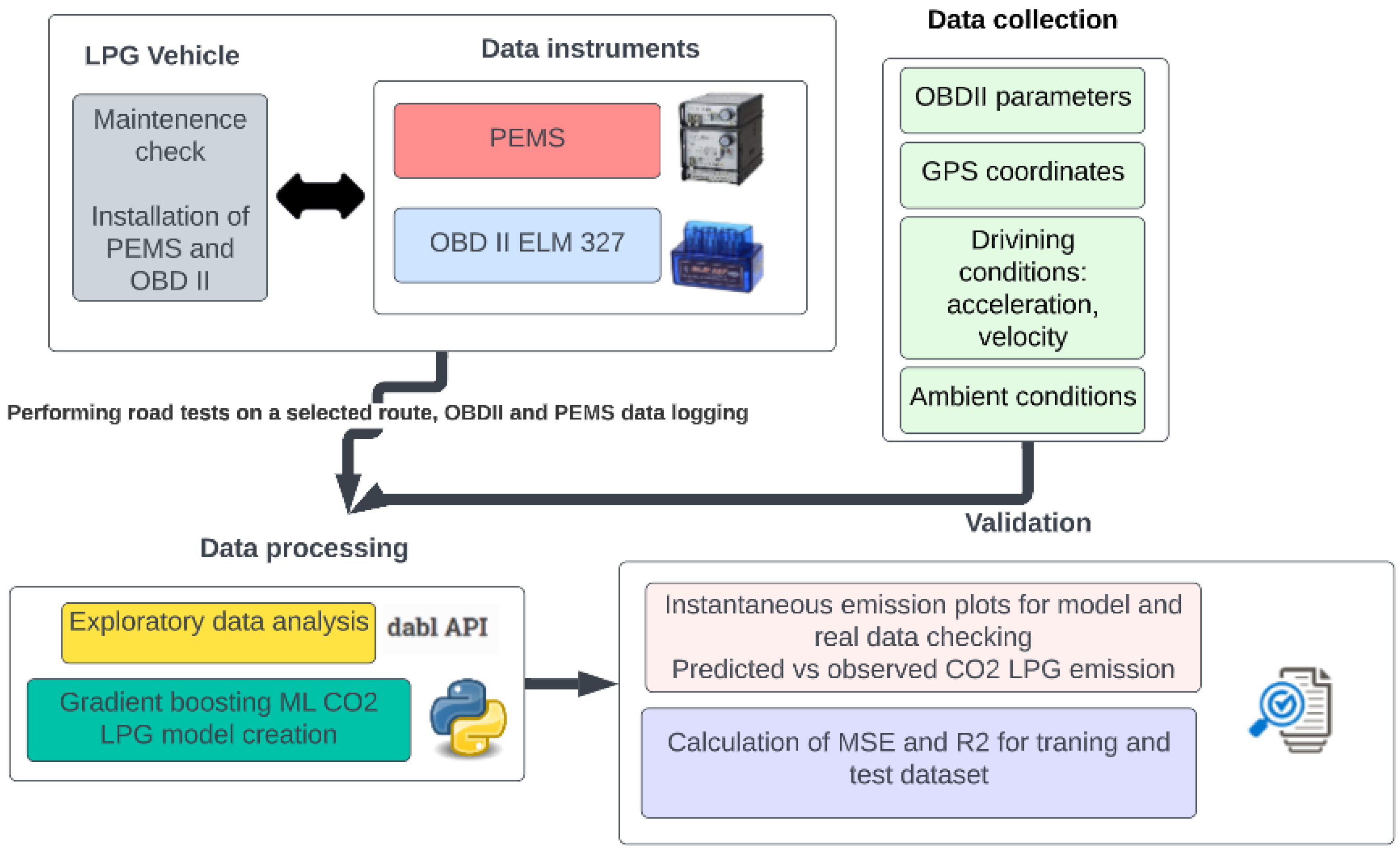
2. Materials and Methods

The general scheme of the work is shown in Figure 1. The work consisted of collecting data from the LPG vehicle from the PEMS system and the OBDII interface. These data were aggregated on a computer connected to these systems. After aggregation, the data were then subjected to EDA to select the best set of predictors to create a CO2 emission model for the LPG vehicle. The model was made in a Python environment using the gradient boosting method. Validation of the model was conducted by analysing the instantaneous emissions, predicted vs. observed plots, and calculating the MSE and R2 ratios.
The work involved driving through the road in different parts of the conurbation in order to collect a large amount of data for different traffic conditions. The journeys were carried out using the PEMS, which was installed in the test vehicle. The PEMS test apparatus is a Horiba OBS-2200, which can measure the instantaneous emissions of CO2, CO, THC, and NOx. It is equipped with a flame ionization detector (FID) to measure THC, non-dispersive infrared spectrometer (NDIR) to measure CO and CO2, and a chemiluminescence detector (CLD) for measuring NO and NO2 [30]. In order to avoid condensation on the line sending the exhaust gas sample from the vehicle’s exhaust system to the PEMS system, the PEMS controller heats it to 190 °C [31]. The PEMS is additionally equipped with GPS data, temperature, and ambient humidity measurements. During the road tests, the vehicle was powered exclusively with LPG fuel. The focus of this study was on the analysis and modelling of CO2 emissions.
The vehicle under study was manufactured in 2014 (Euro 6), has a 1397 cc engine, spark ignition type, and its main fuel is gasoline; while it is possible to run to the factory LPG system, the maximum power is 55 kW for 5500 RPM, the maximum torque is 105 Nm for 4250 RPM, it has manual transmission and 5 gears, the after-treatment system is TWC, and the weight of the vehicle is 980 kg. A diagram of the vehicle under test, including the location of the sensors and the OBDII interface, is shown in Figure 2.
The survey route is shown in Figure 3. The surveyed route totals 115 km, while its structure contains driving sections characteristic of the urban, rural, and motorway parts. This choice of route was conditioned by the collection of a large number of data for different traffic conditions of the vehicle, taking into account different speed ranges; for example, for the urban part, the distribution of speed data was between 0 and 60 km/h, while for the other parts of the road, the driving speeds were higher than 60 km/h.
The data from the journeys were recorded on a computer, which read the input from the PEMS system for the amount of exhaust gas flowing, CO2 concentration, exhaust gas temperature, ambient temperature, and the vehicle location, which was then used to determine the CO2 emissions recorded in g/s. Furthermore, an ELM327 interface was connected to the vehicle to record OBDII data, while the parameters recorded were engine rpm, throttle position, engine load, acceleration, turbo boost and vacuum gauge, altitude, and velocity. Data for both PEMS and OBDII were recorded at a frequency of every 1 s.

3. Results

3.1. Exploratory PEMS and OBDII Data Analysis for the LPG-Fuelled Vehicle

For the road test data obtained from the PEMS and the OBDII interface, EDA was carried out in the first stage of the work so a set of best predictive parameters could be correlated to estimate CO2 emissions from an LPG vehicle. Exploratory data analysis is a process which allows one to understand the data and discover certain patterns, correlations, and anomalies [32,33]. In the context of creating machine learning models as elements of artificial intelligence techniques, EDA allows for in-depth analysis and identification of potential problems that need to be performed prior to the model-building process. The essence of performing EDA in the context of creating machine learning models has been described in the work [34].
The EDA was performed using the Python environment in the dabl library. In machine learning, we can divide the data into two main categories: targets and features. Features are input data that are used as predictors, whereas target data are output data, most often a single variable. In machine learning algorithms, continuous type variables are often encountered [35,36]. For the case studied, the characteristic variables were all data collected from the OBDII interface, while the target variable was the CO2 emissions measured with the PEMS system. A graph showing these variables is shown in Figure 4.
In Figure 4, the continuous feature vs. the target derived from the OBDII interface and the PEMS can be observed, particularly: engine speed (Engine RPM), throttle position (%), engine load (%), acceleration (m/s2), turbo boost and vacuum gauge (psi), altitude (m), and velocity (km/h). From Figure 4, the following can be observed:
-
The positive correlation of the CO2 emissions parameter with engine RPM and vehicle speed;
-
No correlation or small correlation of CO2 emissions with engine load, acceleration, turbo boost, vacuum gauge, and altitude.
Based on the above observations, the best explanatory variables to model CO2 emissions with recorded parameters would be the RPM of the engine and the vehicle speed. To verify this, a Pearson’s correlation coefficient was additionally calculated to numerically verify the above observations. In the context of the development of machine learning models, the Pearson’s correlation coefficient can be used to quantify the correlation between the variables under study and the target variable. The results of the Pearson’s correlation coefficient for the parameters studied are presented in Figure 5.
From Figure 5, the following can be observed:
-
The highest values of Pearson’s coefficient correlation with CO2 emissions are found for the parameter’s velocity—0.68; engine RPM—0.72; and throttle position—0.63,
-
The least correlated parameters with CO2 emissions are acceleration—0.19 and altitude—0.11.
The results of the Pearson’s correlation coefficient for the tested parameters of PEMS and OBDII confirmed the earlier visual analyses for the continuous feature vs. the target CO2 emission graphs. The variables chosen as explanatory variables were velocity and engine RPM.

3.2. Creation of CO2 Emission Models for the Vehicle Fuelled with LPG

CO2 emissions from a vehicle that runs on LPG are lower than those of the same vehicle that runs on, for example, gasoline [37]. This is despite the fact that the volumetric consumption of an LPG engine is 15 to 20 percent higher than that of petrol engines [38,39]. The lack or small number of emission models for this type of power supply, mainly on a microscale, creates the need for this type of computational model. One of the methods currently used to model emissions is artificial intelligence techniques. Machine learning is a subfield of artificial intelligence that uses statistical techniques and algorithms which allow computer systems to improve the modelling performance [40,41]. Machine learning algorithms are most commonly implemented using programming languages such as R and Python, while popular libraries used for this purpose include TensorFlow, Keras, and Scikit-learn [42,43,44]. The process of creating a vehicle emissions model includes collecting data during different driving states along the route under study. These data can also be collected under laboratory conditions in a more controlled environment.
To create a CO2 emissions model for an LPG vehicle, parameters such as velocity and engine RPM were used as explanatory variables. Often in the context of emission models, parameters such as velocity, acceleration, and road gradient are chosen for their creation [45]. However, as the EDA conducted earlier for the collected data shows, these variables do not always have the best influence on the final result of the emission model.
The PEMS and OBDII data obtained from the road test were saved in.csv format and uploaded to the Github data repository. Github is a platform to store and manage files and code, among other things, in a centralised location which allows these data to be shared and contribute to open-source projects [46]. The data were then downloaded to code on the Google Colab cloud platform, which enables the creation and running of projects based on Jupyter notebook-based projects [47]. Jupyter notebooks are a popular tool used in data science and machine learning, allowing users to create and share interactive documents that combine code, text, and visualisations.
The machine learning techniques chosen to create a model for CO2 emissions from an LPG vehicle were linear regression, random forest, support vector machine, and gradient boosting. The validation of the resulting models was carried out using MSE and R2. The best results were obtained with the gradient boosting technique, so only the results for this machine learning technique are presented in this section.
The creation of the model began by dividing the data set into two subsets: the model training set, which accounted for 80% of all data obtained during the test, and the test set, which accounted for 20%. Subsequent sets of models were then imported into the sklearn library to create predictions. The main codes used to prepare the emission models are presented in the Algorithm 1.
Algorithm 1. LPG vehicle emission model in Python; selected codes.
  • df = pd.read_csv (‘LPG data path) #indicating path for the data set
  • from sklearn.model_selection import train_test_split
    X_train, X_test, y_train, y_test = train_test_split(X,y, test_size = 0.2, random_state = 100) # division of data for test and train set
  • from sklearn.ensemble import GradientBoostingRegressor
    gb = GradientBoostingRegressor(random_state = 0)
    gb.fit(X_train, y_train) # importing gradientboosting model from sklearn
  • y_gb_train_pred = gb.predict (X_train)
    y_gb_test_pred=gb.predict(X_test) #applying the model to make predictions
  • from sklearn.metrics import mean_squared_error, r2_score
    gb_train_mse = mean_squared_error(y_train, y_gb_train_pred)
    gb_train_r2 = r2_score(y_train, y_gb_train_pred)
    gb_test_mse = mean_squared_error(y_test, y_gb_test_pred)
    gb_test_r2 = r2_score(y_test, y_gb_test_pred) # Evaluation of the model performance
The scikit-learn library was used to create a model of CO2 emissions from an LPG vehicle. A graph showing the speed and engine RPM parameters for the test route is presented in Figure 6.

3.3. Validation of a CO2 Emission Model for an LPG Vehicle

Validation of a machine learning model is the process of evaluating the estimates of the results from the model to the results for the data set under study [48]. For the case study, the validation was carried out by comparing the model results with the on-road results for instantaneous CO2 emissions with an LPG vehicle, for the total emissions results for the route under study, and to evaluate the CO2 emission estimates for the aggregation of data for different driving speeds. The validation of the machine learning model is an essential step as it allows us to assess the accuracy of the obtained model and its estimation capability for new data. The mean square error (MSE) and R2 were used for both the training and the test data to quantitatively validate the results obtained.
The verification of the CO2 model for an LPG vehicle against the actual road emissions is shown in Figure 7. The model results are presented for the gradient boost technique, as this is the technique for which the best CO2 emission mapping results were obtained for the LPG vehicle under test. Gradient boosting is a popular machine learning method for supervised learning tasks, both for classification and regression. It is an ensemble method that combines multiple weak models to create a strong predictive model. The gradient boosting method is based on the addition of new models to the ensemble and each model tries to correct the errors of the previous model.
In Figure 7, we can see how the actual CO2 emissions of an LPG vehicle and the modelled emissions compare. For certain areas, especially at the beginning of the test, where there is a certain area for the so-called “cold start” phenomenon, we can observe a certain underestimation of the vehicle’s CO2 emission results. A cold start of the vehicle may last for up to several minutes until the engine reaches its expected optimum operating temperature, which is around 80–90 °C [49]. During this time, the vehicle’s fuel consumption may be higher than normal [50]. This phenomenon is due to the fact that when the vehicle’s engine is cold, the fuel mixture is richer than normal, which can cause the fuel injected into the combustion chamber to be in greater quantities than required [51]. This excess fuel allows the engine to start smoothly, but the result is a higher fuel consumption, which also directly translates into higher CO2 emissions. After a period of time, when the engine has reached its optimum operating temperature, we can observe that the model makes more accurate predictions. There are some areas of underestimation, but, overall, if we consider the behaviour and the prediction of the model, it is both good. This is also confirmed by the sum of emissions from the road test and the model. The sum of emissions for the above test for the actual data was 3386 g CO2, while for the model data it was 3379 g.
Figure 8 shows the predicted vs. observed CO2 emission of the LPG vehicle. It serves the purpose of comparing the results obtained from the machine learning model with the actual results. The shape of this graph gives valuable information about the performance of the obtained machine learning model. Data, especially in the area of emissions of up to 3 g/s CO2, are located close to the line. Higher emission values of 3 to 6 g/s are also relatively close to the centre of the line, defining a good fit.
Figure 9 shows a graph of CO2 emissions from an LPG vehicle using model data and actual data from a road test. The CO2 emission results in the graph are plotted against the vehicle speed. The results were arranged relative to increasing speed in order to verify the model estimates for different speed values. From this graph, we can observe that the model better represents the CO2 emissions for driving speeds between 0 and 50 km/h, which may be due to the fact that more data were collected for these driving conditions. Speeds are characteristic of driving in the urban part of the route. For higher speeds, the graph of modelled CO2 emissions creates points for the average emissions that are obtained for such driving characteristics.
For quantitative metrics, R2 and MSE were used to validate the CO2 emissions model for an LPG vehicle. The coefficient of determination is a statistical measure that is commonly used to validate machine learning models [52,53]. R2 is calculated as the ratio of the explained variation in the target variable to the total variation in the target variable. The second measure used was the mean squared error, which is also a common indicator that is used to validate and evaluate the performance of regression models [54]. The MSE is calculated by taking the average of the squared differences between the predicted and actual values of the target variable across all data points in the training set [55]. The results of the model validation indices are presented in Table 1. The results of the indices obtained for both the training and test data sets show that the representation of the model data relative to the actual data is satisfactory and that the resulting CO2 model can be used for emission prediction on new data sets.

4. Discussion

By analysing the results obtained from the CO2 emission model for an LPG vehicle, some advantages and disadvantages can be observed:
  • An advantage of the model is the very good overall predictive ability of the instantaneous CO2 emissions from the LPG vehicle, especially for speeds up to 50 km/h,
  • A disadvantage of the model obtained is some erroneous results of instantaneous CO2 emissions for the cold start period of the engine, where we can observe increased fuel consumption, resulting in higher-than-normal CO2 emissions.
Therefore, it is necessary to create an additional CO2 emission model for the thermal state emissions. This will undoubtedly become the subject of further development work on emissions modelling for LPG vehicles. The creation of models for cold starts is the subject of, inter alia, the work [56,57,58], in which the authors indicate recommendations for separate emission modelling for this thermal state of the vehicle.
The resulting model also gives a very good estimate of the total CO2 emissions for a given route with a very small margin of error. It is also important to note that the modelling itself was performed on the basis of a prior analysis of a set of potential explanatory variables from PEMS and OBDII.
Furthermore, when comparing the model results with other work, it can be seen that this is one of the first models of instantaneous CO2 emissions on a microscale for an LPG vehicle. Other examples of work that has investigated similar topics include the work from [59]. This work describes the actual emissions of LPG-powered taxis. The emissions measurements in this work relate to CO, HC, and NOx emissions. These results were correlated with emission factors with instantaneous vehicle speeds and acceleration profile parameters for local urban driving patterns. The aim of this work, however, was to determine how replacing a fleet of diesel taxis with LPG taxis could reduce emissions. Another article that addresses the emissions of LPG vehicles is [60]. However, this work is limited only to a comparison of emission factors for a vehicle at idle speed. Another article that addresses emissions from vehicles running on LPG, among other fuels, is [61]. Remote sensing measurements collected over three different periods were used to study vehicle gas emissions. The gaseous emission factors of petrol and LPG vehicles increase rapidly within two years of being introduced to the fleet, suggesting that the engine and catalyst performance degrade rapidly. Another example of the work that considers the emissions of LPG vehicles in its research is [62]. This article compares hybrid electric, LPG, and petrol vehicles with a Life Cycle Assessment (LCA) approach.
In terms of the methods used, there are also a small number of works that use the OBDII interface and the PEMS system in modelling vehicle emissions. One example that uses OBDII data to model vehicle fuel consumption is the work in [63]. This work used variables from the OBD system, such as RPM and SVM, to prepare a model using the support vector machine technique. However, using only the OBDII interface to load the vehicle’s fuel consumption data may lead to a poor estimation of the vehicle’s actual consumption, as often the vehicle controller does not provide such information as the actual fuel consumption, while the programme itself, which loads the OBDII data, calculates this fuel consumption computationally.
In the context of the use of artificial intelligence computing techniques, particularly machine learning, their popularity is growing. There is a range of software and environments for creating such models. Frequently used in this context are the MATLAB [64] and Python [65,66] programming environments. The resulting emission calculation models can provide reliable and accurate results and can be used to support decision-making processes at the level of, for example, road management in the context of environmental protection.

5. Conclusions

The literature review carried out showed that there is no micro-scale emissions model for estimating CO2 for an LPG vehicle. Therefore, this paper presents the process of creating a CO2 emissions model for an LPG vehicle. The model created was based on data from the PEMS system and the OBDII interface. The best method for predicting CO2 for an LPG vehicle proved to be the machine learning gradient boosting method. As a result of the EDA conducted, two variables were selected as a set of predictors: speed and engine rpm. The obtained results of the model for the indicator for the R2 test—0.61 and the MSE test—0.77 indicate a good representation of the model data for future predicates. The model created, in particular, predicts CO2 emissions well for speeds characteristic of driving in an urban area. The estimation of the total on-road CO2 emissions from the LPG vehicle is also very accurate—for the data analysed it was 3386 g for the actual data, while for the model data it was 3379 g.
The limitations of the work are that the road data set was carried out for only one LPG vehicle, so this aspect should be considered at the same time for further work on the topic under study. It is also important to take into account, when creating new models, the emission data for the so-called “cold start” of the engine, as they are different from those when the vehicle engine is warmed up. To solve this problem, it is important to exclude data for the cold start phase and to create a separate CO2 emissions model. As a result of the literature review, attention should also be paid to the change in the condition of the catalytic converters of LPG vehicles, especially with the passage of years, so the development of an emission model for LPG vehicles should take into account the continuous updating of the emission data for the vehicles which are included in the model. The methodology presented in this paper for modelling LPG vehicle emissions may be scalable to other cases of vehicle emissions modelling.

Funding

This work was supported by the Ministry of Infrastructure and Development as part of the Eastern Poland Development Operational Program in association with the European Regional Development Fund, which financed the research instruments.

Data Availability Statement

Data are accessible under the following link: https://github.com/MaksMadz/MDPI---LPG-data/blob/4f151efa70e16dbf0443df020a99ebd62461dd9d/DataMDPILPG.csv (accessed on 28 February 2023); in case of questions, more data can be shared.

Conflicts of Interest

The authors declare no conflict of interest.

Nomenclature

COCarbon monoxide
CO2Carbon dioxide
EDAExploratory data analysis
EEAEuropean Environment Agency
GHGGreenhouse gas
LCALife Cycle Assessment
LPGLiquefied petroleum gas
MSEMean squared error
NOxNitrogen oxides
OBDOn-board diagnostic
PEMSPortable emission measurement system
R2Coefficient of determination
SVMSupport vector machine
THCTotal hydrocarbon

References

  1. Panchasara, H.; Samrat, N.H.; Islam, N. Greenhouse gas emissions trends and mitigation measures in australian agriculture sector—A review. Agriculture 2021, 11, 85. [Google Scholar] [CrossRef]
  2. Mądziel, M.; Campisi, T. Investigation of Vehicular Pollutant Emissions at 4-Arm Intersections for the Improvement of Integrated Actions in the Sustainable Urban Mobility Plans (SUMPs). Sustainability 2023, 15, 1860. [Google Scholar] [CrossRef]
  3. Hao, H.; Mu, Z.; Jiang, S.; Liu, Z.; Zhao, F. GHG Emissions from the production of lithium-ion batteries for electric vehicles in China. Sustainability 2017, 9, 504. [Google Scholar] [CrossRef] [Green Version]
  4. Neagu, O.; Teodoru, M.C. The relationship between economic complexity, energy consumption structure and greenhouse gas emission: Heterogeneous panel evidence from the EU countries. Sustainability 2019, 11, 497. [Google Scholar] [CrossRef] [Green Version]
  5. Fuinhas, J.A.; Koengkan, M.; Leitão, N.C.; Nwani, C.; Uzuner, G.; Dehdar, F.; Relva, S.; Peyerl, D. Effect of battery electric vehicles on greenhouse gas emissions in 29 European Union countries. Sustainability 2021, 13, 13611. [Google Scholar] [CrossRef]
  6. Jiang, R.; Wu, P.; Wu, C. Driving factors behind energy-related carbon emissions in the US road transport sector: A decomposition analysis. Int. J. Environ. Res. Public Health 2022, 19, 2321. [Google Scholar] [CrossRef] [PubMed]
  7. Brown, T.; Schäfer, M.; Greiner, M. Sectoral interactions as carbon dioxide emissions approach zero in a highly-renewable European energy system. Energies 2019, 12, 1032. [Google Scholar] [CrossRef] [Green Version]
  8. Stoilova, S.; Munier, N.; Kendra, M.; Skrúcaný, T. Multi-criteria evaluation of railway network performance in countries of the TEN-T orient–east med corridor. Sustainability 2020, 12, 1482. [Google Scholar] [CrossRef] [Green Version]
  9. Selleri, T.; Melas, A.D.; Joshi, A.; Manara, D.; Perujo, A.; Suarez-Bertoa, R. An overview of lean exhaust deNOx aftertreatment technologies and NOx emission regulations in the European union. Catalysts 2021, 11, 404. [Google Scholar] [CrossRef]
  10. Haas, T.; Sander, H. Decarbonizing transport in the European Union: Emission performance standards and the perspectives for a European Green Deal. Sustainability 2020, 12, 8381. [Google Scholar] [CrossRef]
  11. Veludo, G.; Cunha, M.; Sá, M.M.; Oliveira-Silva, C. Offsetting the Impact of CO2 Emissions Resulting from the Transport of Maiêutica’s Academic Campus Community. Sustainability 2021, 13, 10227. [Google Scholar] [CrossRef]
  12. Lajunen, A.; Kivekäs, K.; Vepsäläinen, J.; Tammi, K. Influence of increasing electrification of passenger vehicle fleet on carbon dioxide emissions in Finland. Sustainability 2020, 12, 5032. [Google Scholar] [CrossRef]
  13. Leal Filho, W.; Abubakar, I.R.; Kotter, R.; Grindsted, T.S.; Balogun, A.L.; Salvia, A.L.; Aina, Y.; Wolf, F. Framing electric mobility for urban sustainability in a circular economy context: An overview of the literature. Sustainability 2021, 13, 7786. [Google Scholar] [CrossRef]
  14. Šarkan, B.; Jaśkiewicz, M.; Kubiak, P.; Tarnapowicz, D.; Loman, M. Exhaust emissions measurement of a vehicle with retrofitted LPG system. Energies 2022, 15, 1184. [Google Scholar] [CrossRef]
  15. Jaworski, A.; Mądziel, M.; Kuszewski, H.; Lejda, K.; Balawender, K.; Jaremcio, M.; Jakubowski, M.; Woś, P.; Lew, K. The Impact of Driving Resistances on the Emission of Exhaust Pollutants from Vehicles with the Spark Ignition Engine Fuelled by Petrol and LPG; SAE Technical Paper; SAE International: Warrendale, PA, USA, 2020. [Google Scholar]
  16. Hollada, J.; Williams, K.N.; Miele, C.H.; Danz, D.; Harvey, S.A.; Checkley, W. Perceptions of improved biomass and liquefied petroleum gas stoves in Puno, Peru: Implications for promoting sustained and exclusive adoption of clean cooking technologies. Int. J. Environ. Res. Public Health 2017, 14, 182. [Google Scholar] [CrossRef] [Green Version]
  17. Warguła, Ł.; Kukla, M.; Lijewski, P.; Dobrzyński, M.; Markiewicz, F. Influence of the use of Liquefied Petroleum Gas (LPG) systems in woodchippers powered by small engines on exhaust emissions and operating costs. Energies 2020, 13, 5773. [Google Scholar] [CrossRef]
  18. Usman, M.; Farooq, M.; Naqvi, M.; Saleem, M.W.; Hussain, J.; Naqvi, S.R.; Jahangir, S.; Usama, H.M.J.; Idrees, S.; Anukam, A. Use of gasoline, LPG and LPG-HHO blend in SI engine: A comparative performance for emission control and sustainable environment. Processes 2020, 8, 74. [Google Scholar] [CrossRef] [Green Version]
  19. Brzezińska, D. LPG cars in a car park environment—How to make it safe. Int. J. Environ. Res. Public Health 2019, 16, 1062. [Google Scholar] [CrossRef] [Green Version]
  20. Jena, P.R.; Managi, S.; Majhi, B. Forecasting the CO2 emissions at the global level: A multilayer artificial neural network modelling. Energies 2021, 14, 6336. [Google Scholar] [CrossRef]
  21. Giechaskiel, B.; Lähde, T.; Clairotte, M.; Suarez-Bertoa, R.; Valverde, V.; Melas, A.D.; Selleri, T.; Bonnel, P. Emissions of Euro 6 Mono-and Bi-Fuel Gas Vehicles. Catalysts 2022, 12, 651. [Google Scholar] [CrossRef]
  22. Paczuski, M.; Marchwiany, M.; Puławski, R.; Pankowski, A.; Kurpiel, K.; Przedlacki, M. Liquefied Petroleum Gas (LPG) as a Fuel for Internal Combustion Engines; Alternative fuels, technical and environmental conditions; InTechOpen: London, UK, 2016; Volume 13. [Google Scholar]
  23. Aydin, M.; Irgin, A.; Çelik, M.B. The impact of diesel/LPG dual fuel on performance and emissions in a single cylinder diesel generator. Appl. Sci. 2018, 8, 825. [Google Scholar] [CrossRef] [Green Version]
  24. Cardone, M.; Marialto, R.; Ianniello, R.; Lazzaro, M.; Di Blasio, G. Spray analysis and combustion assessment of diesel-LPG fuel blends in compression ignition engine. Fuels 2020, 2, 1–15. [Google Scholar] [CrossRef]
  25. Li, F.; Zhuang, J.; Cheng, X.; Li, M.; Wang, J.; Yan, Z. Investigation and prediction of heavy-duty diesel passenger bus emissions in Hainan using a COPERT model. Atmosphere 2019, 10, 106. [Google Scholar] [CrossRef] [Green Version]
  26. Mądziel, M.; Campisi, T. Assessment of vehicle emissions at roundabouts: Acomparative study of PEMS data and microscale emission model. Arch. Transp. 2022, 63, 35–51. [Google Scholar] [CrossRef]
  27. Ali, M.; Kamal, M.D.; Tahir, A.; Atif, S. Fuel consumption monitoring through COPERT model—A case study for urban sustainability. Sustainability 2021, 13, 11614. [Google Scholar] [CrossRef]
  28. Obaid, M.; Torok, A.; Ortega, J. A comprehensive emissions model combining autonomous vehicles with park and ride and electric vehicle transportation policies. Sustainability 2021, 13, 4653. [Google Scholar] [CrossRef]
  29. Zhang, R.; Wang, Y.; Pang, Y.; Zhang, B.; Wei, Y.; Wang, M.; Zhu, R. A Deep Learning Micro-Scale Model to Estimate the CO2 Emissions from Light-Duty Diesel Trucks Based on Real-World Driving. Atmosphere 2022, 13, 1466. [Google Scholar] [CrossRef]
  30. Rodman Oprešnik, S.; Seljak, T.; Vihar, R.; Gerbec, M.; Katrašnik, T. Real-world fuel consumption, fuel cost and exhaust emissions of different bus powertrain technologies. Energies 2018, 11, 2160. [Google Scholar] [CrossRef] [Green Version]
  31. Lejda, K.; Jaworski, A.; Mądziel, M.; Balawender, K.; Ustrzycki, A.; Savostin-Kosiak, D. Assessment of petrol and natural gas vehicle carbon oxides emissions in the laboratory and on-road tests. Energies 2021, 14, 1631. [Google Scholar] [CrossRef]
  32. Bezerra, A.; Silva, I.; Guedes, L.A.; Silva, D.; Leitão, G.; Saito, K. Extracting value from industrial alarms and events: A data-driven approach based on exploratory data analysis. Sensors 2019, 19, 2772. [Google Scholar] [CrossRef] [Green Version]
  33. Taboada, G.L.; Han, L. Exploratory data analysis and data envelopment analysis of urban rail transit. Electronics 2020, 9, 1270. [Google Scholar] [CrossRef]
  34. Mądziel, M.; Campisi, T. Energy Consumption of Electric Vehicles: Analysis of Selected Parameters Based on Created Database. Energies 2023, 16, 1437. [Google Scholar] [CrossRef]
  35. Nabipour, M.; Nayyeri, P.; Jabani, H.; Shahab, S.; Mosavi, A. Predicting stock market trends using machine learning and deep learning algorithms via continuous and binary data; a comparative analysis. IEEE Access 2020, 8, 150199–150212. [Google Scholar] [CrossRef]
  36. Mothilal, R.K.; Sharma, A.; Tan, C. Explaining machine learning classifiers through diverse counterfactual explanations. In Proceedings of the 2020 Conference on Fairness, Accountability, and Transparency, Barcelona, Spain, 27–30 January 2020; pp. 607–617. [Google Scholar]
  37. Demirbas, A. Fuel properties of hydrogen, liquefied petroleum gas (LPG), and compressed natural gas (CNG) for transportation. Energy Sources 2002, 24, 601–610. [Google Scholar] [CrossRef]
  38. Saraf, R.R.; Thipse, S.S.; Saxena, P.K. Experimental Performance Analysis of LPG/Gasoline Bi-Fuel Passenger Car PFI Engines (No. 2007-01-2132); SAE Technical Paper; SAE International: Warrendale, PA, USA, 2007. [Google Scholar]
  39. Tasic, T.; Pogorevc, P.; Brajlih, T. Gasoline and LPG exhaust emissions comparison. Adv. Prod. Eng. Manag. 2011, 6, 87–94. [Google Scholar]
  40. Cioffi, R.; Travaglioni, M.; Piscitelli, G.; Petrillo, A.; De Felice, F. Artificial intelligence and machine learning applications in smart production: Progress, trends, and directions. Sustainability 2020, 12, 492. [Google Scholar] [CrossRef] [Green Version]
  41. Lowe, M.; Qin, R.; Mao, X. A review on machine learning, artificial intelligence, and smart technology in water treatment and monitoring. Water 2022, 14, 1384. [Google Scholar] [CrossRef]
  42. Ak, M.F. A comparative analysis of breast cancer detection and diagnosis using data visualization and machine learning applications. Healthcare 2020, 8, 111. [Google Scholar] [CrossRef]
  43. Maxwell, A.E.; Pourmohammadi, P.; Poyner, J.D. Mapping the topographic features of mining-related valley fills using mask R-CNN deep learning and digital elevation data. Remote Sens. 2020, 12, 547. [Google Scholar] [CrossRef] [Green Version]
  44. Li, K.Y.; de Lima, R.S.; Burnside, N.G.; Vahtmäe, E.; Kutser, T.; Sepp, K.; Pinheiro, V.H.C.; Yang, M.-D.; Vain, A.; Sepp, K. Toward automated machine learning-based hyperspectral image analysis in crop yield and biomass estimation. Remote Sens. 2022, 14, 1114. [Google Scholar] [CrossRef]
  45. Jaworski, A.; Mądziel, M.; Lejda, K. Creating an emission model based on portable emission measurement system for the purpose of a roundabout. Environ. Sci. Pollut. Res. 2019, 26, 21641–21654. [Google Scholar] [CrossRef] [PubMed] [Green Version]
  46. Liao, Z.; Yi, M.; Wang, Y.; Liu, S.; Liu, H.; Zhang, Y.; Zhou, Y. Healthy or not: A way to predict ecosystem health in github. Symmetry 2019, 11, 144. [Google Scholar] [CrossRef] [Green Version]
  47. Ray, S.; Alshouiliy, K.; Agrawal, D.P. Dimensionality reduction for human activity recognition using google colab. Information 2020, 12, 6. [Google Scholar] [CrossRef]
  48. Istiaque Ahmed, K.; Tahir, M.; Hadi Habaebi, M.; Lun Lau, S.; Ahad, A. Machine learning for authentication and authorization in iot: Taxonomy, challenges and future research direction. Sensors 2021, 21, 5122. [Google Scholar] [CrossRef]
  49. Jaworski, A.; Mądziel, M.; Kuszewski, H.; Lejda, K.; Balawender, K.; Jaremcio, M.; Jakubowski, M.; Wojewoda, P.; Lew, K.; Ustrzycki, A. Analysis of Cold Start Emission from Light Duty Vehicles Fueled with Gasoline and LPG for Selected Ambient Temperatures; SAE Technical Paper; SAE International: Warrendale, PA, USA, 2020. [Google Scholar]
  50. Hu, J.; Frey, H.C.; Boroujeni, B.Y. Contribution of Cold Starts to Real-World Trip Emissions for Light-Duty Gasoline Vehicles. Atmosphere 2022, 14, 35. [Google Scholar] [CrossRef]
  51. Frey, H.C.; Zheng, X.; Hu, J. Variability in measured real-world operational energy use and emission rates of a plug-in hybrid electric vehicle. Energies 2020, 13, 1140. [Google Scholar] [CrossRef] [Green Version]
  52. Ziółkowski, J.; Oszczypała, M.; Małachowski, J.; Szkutnik-Rogoż, J. Use of artificial neural networks to predict fuel consumption on the basis of technical parameters of vehicles. Energies 2021, 14, 2639. [Google Scholar] [CrossRef]
  53. Fang, S.; Tang, W.; Peng, Y.; Gong, Y.; Dai, C.; Chai, R.; Liu, K. Remote estimation of vegetation fraction and flower fraction in oilseed rape with unmanned aerial vehicle data. Remote Sens. 2016, 8, 416. [Google Scholar] [CrossRef] [Green Version]
  54. Li, Z.; Rahman, S.M.; Vega, R.; Dong, B. A hierarchical approach using machine learning methods in solar photovoltaic energy production forecasting. Energies 2016, 9, 55. [Google Scholar] [CrossRef] [Green Version]
  55. Nguyen, V.V.; Pham, B.T.; Vu, B.T.; Prakash, I.; Jha, S.; Shahabi, H.; Shirzadi, A.; Ba, D.N.; Kumar, R.; Chatterjee, J.M.; et al. Hybrid machine learning approaches for landslide susceptibility modeling. Forests 2019, 10, 157. [Google Scholar] [CrossRef] [Green Version]
  56. Jeanneret, B.; Guille Des Buttes, A.; Pelluet, J.; Keromnes, A.; Pélissier, S.; Le Moyne, L. Optimal Control of a Spark Ignition Engine Including Cold Start Operations for Consumption/Emissions Compromises. Appl. Sci. 2021, 11, 971. [Google Scholar] [CrossRef]
  57. Han, D.; Jiaqiang, E.; Deng, Y.; Chen, J.; Leng, E.; Liao, G.; Zhao, X.; Feng, C.; Zhang, F. A review of studies using hydrocarbon adsorption material for reducing hydrocarbon emissions from cold start of gasoline engine. Renew. Sustain. Energy Rev. 2021, 135, 110079. [Google Scholar] [CrossRef]
  58. Zare, A.; Bodisco, T.A.; Jafari, M.; Verma, P.; Yang, L.; Babaie, M.; Rahman, M.M.; Banks, A.; Ristovski, Z.D.; Brown, R.J.; et al. Cold-start NOx emissions: Diesel and waste lubricating oil as a fuel additive. Fuel 2021, 286, 119430. [Google Scholar] [CrossRef]
  59. Ning, Z.; Chan, T.L. On-road remote sensing of liquefied petroleum gas (LPG) vehicle emissions measurement and emission factors estimation. Atmos. Environ. 2007, 41, 9099–9110. [Google Scholar] [CrossRef]
  60. Aosaf, M.R.; Wang, Y.; Du, K. Comparison of the emission factors of air pollutants from gasoline, CNG, LPG and diesel fueled vehicles at idle speed. Environ. Pollut. 2022, 305, 119296. [Google Scholar] [CrossRef] [PubMed]
  61. Lau, J.; Hung, W.T.; Cheung, C.S. Observation of increases in emission from modern vehicles over time in Hong Kong using remote sensing. Environ. Pollut. 2012, 163, 14–23. [Google Scholar] [CrossRef] [PubMed] [Green Version]
  62. Boureima, F.-S.; Messagie, M.; Matheys, J.; Wynen, V.; Sergeant, N.; Van Mierlo, J.; De Vos, M.; De Caevel, B. Comparative LCA of electric, hybrid, LPG and gasoline cars in Belgian context. World Electr. Veh. J. 2009, 3, 469–476. [Google Scholar] [CrossRef] [Green Version]
  63. Abukhalil, T.; AlMahafzah, H.; Alksasbeh, M.; Alqaralleh, B.A. Fuel consumption using OBD-II and support vector machine model. J. Robot. 2020, 2020, 50178. [Google Scholar] [CrossRef]
  64. Mądziel, M.; Jaworski, A.; Kuszewski, H.; Woś, P.; Campisi, T.; Lew, K. The Development of CO2 Instantaneous Emission Model of Full Hybrid Vehicle with the Use of Machine Learning Techniques. Energies 2022, 15, 142. [Google Scholar] [CrossRef]
  65. Zha, H.; Miao, Y.; Wang, T.; Li, Y.; Zhang, J.; Sun, W.; Feng, Z.; Kusnierek, K. Improving unmanned aerial vehicle remote sensing-based rice nitrogen nutrition index prediction with machine learning. Remote Sens. 2020, 12, 215. [Google Scholar] [CrossRef] [Green Version]
  66. Quang Tran, D.; Bae, S.H. Proximal policy optimization through a deep reinforcement learning framework for multiple autonomous vehicles at a non-signalized intersection. Appl. Sci. 2020, 10, 5722. [Google Scholar] [CrossRef]
Figure 1. Basic logic and scheme of the performed research.
Energies 16 02754 g001
Figure 2. PEMS platform installed in the vehicle in the study.
Energies 16 02754 g002
Figure 3. Route tested of an LPG vehicle.
Energies 16 02754 g003
Figure 4. Continuous feature vs. target CO2 emission; PEMS and OBDII data for LPG vehicle, the higher the value for F, the better the correlation of the test parameter with CO2 emissions.
Energies 16 02754 g004
Figure 5. Pearson’s correlation coefficient results for the LPG vehicle parameters tested.
Energies 16 02754 g005
Figure 6. Velocity and engine RPM obtained during road test for the LPG-fuelled vehicle.
Energies 16 02754 g006
Figure 7. Instantaneous emission of CO2 using LPG vehicles for model and road data.
Energies 16 02754 g007
Figure 8. Predicted vs. observed CO2 emission from LPG vehicle.
Energies 16 02754 g008
Figure 9. Instantaneous CO2 emissions from an LPG vehicle for model data (blue) and actual data (orange) sorted by increasing vehicle speed (black line) for the entire test run.
Energies 16 02754 g009
Table 1. Results of validation of a CO2 emission model using MSE and R2 for the gradient boosting machine learning technique for an LPG vehicle.
Training MSETraining R2Test MSETest R2
0.558890.7182920.7780430.612655
Disclaimer/Publisher’s Note: The statements, opinions and data contained in all publications are solely those of the individual author(s) and contributor(s) and not of MDPI and/or the editor(s). MDPI and/or the editor(s) disclaim responsibility for any injury to people or property resulting from any ideas, methods, instructions or products referred to in the content.

