Article

Standard Load Profiles for Electric Vehicle Charging Stations in Germany Based on Representative, Empirical Data

1
Grid Integration and Storage System Analysis, Institute for Power Electronics and Electrical Drives (ISEA), RWTH Aachen University, 52074 Aachen, Germany
2
Institute for Power Generation and Storage Systems (PGS), E.ON ERC, RWTH Aachen University, 52074 Aachen, Germany
3
Juelich Aachen Research Alliance, JARA-Energy, 52056 Aachen, Germany
4
National Research Center for Electric Vehicles, Beijing Institute of Technology, Beijing 100081, China
5
Helmholtz Institute Muenster (HI MS), IEK-12, Forschungszentrum Jülich, 52428 Jülich, Germany
*
Author to whom correspondence should be addressed.
Energies 2023, 16(6), 2619; https://doi.org/10.3390/en16062619
Submission received: 30 January 2023 / Revised: 24 February 2023 / Accepted: 2 March 2023 / Published: 10 March 2023

Abstract

:
Electric vehicles are becoming dominant in the global automobile market due to their better environmental friendliness compared to internal combustion vehicles. An adequate network of public charging stations is required to fulfil the fast charging demands of EV users. Knowing the shape and amplitude of their power curves is essential for power purchase planning and grid capacity sizing. Based on a large-scale empirical and representative dataset, this paper creates standard load profiles for various power levels, station sizes, and operating environments. It is found that the average power per charge point increases with rated station power, particularly for a rated power above 100 kW, and decreases with the number of charge points per station for AC chargers. For AC chargers, it is revealed how the shape of the power curve largely depends on the environment of a station, with urban settings experiencing the highest average power of 0.71 kW on average leading to an annual energy sale of 6.2 MWh. These findings show that the rated grid capacity can be well below the sum of the rated power of each charge point.

1. Introduction

Electric vehicles (EVs) are becoming dominant passenger cars in major automobile markets around the world [1]. Charging infrastructure is needed to refuel the EV fleet and thus plays a vital role in the mass adoption of EVs [2]. While a majority of EV users are able to recharge their vehicles at home or their workplace, public charging stations (PCSs) are required for people without private recharging accessibility or to meet fast charging demands [3]. Given the rapidly increasing number of EVs, the power hike at PCSs becomes a big concern for local grids [4].
Generally, charge point operators (CPOs) need to purchase energy from the electricity market and grid operators need to upgrade the grid capacity to accommodate increased charging loads. For households, one typically synthesises load profiles for different types of dwellings, seasons, days, etc., from historical energy consumption records. These profiles are referred to as standard load profiles [5]. Grid planning and energy purchasing are traditionally performed considering these factors, which are also used to determine the transformer and the power line capacity for a given number of EV users.
However, no such profiles exist for PCSs and only small-scale results or models have been periodically reported for predicting the load profiles brought by EVs’ recharge, focusing on either simultaneity factors [6,7] (also called diversity factors for the inverse concept) or load profiles [8,9,10,11,12,13,14]. For instance, Bollerslev et al. [6] used travel surveys and typical EV recharge curves in combination with a Monte Carlo simulation to derive simultaneity factors. This approach can make full use of highly representative and reliable travel surveys but faces difficulty in modelling plugging behaviours. Hu et al. [11] presented a similar approach that only distinctively incorporated a charging model instead of a set of typical charging curves. But these used models can only represent modellers’ expertise while unknown effects cannot be included. Celli et al. [9] employed a Monte Carlo simulation to model 50 kW charging stations. Given that this work was published in 2014, the derived profiles and models may not apply to current situations. Islam and Mithulananthan [10] presented a statistical model built on various factors that cannot be easily accessible. This can be circumvented by running parameter sweeps but at the expense of losing the representativeness of the synthesised load profiles.
Another focal topic in literature is the simulation-based approaches. On this regard, Held et al. [7] focused on the grid’s impacts and performed a power flow simulation, and a charging model was developed based on an assumed EV stock and simulation data. Analogously, Mitrakoudis and Alexiadis [8] also used vehicle stock data and a number of assumptions regarding battery capacity, energy consumption, and charging behaviours derived from different datasets. But they did not disclose the data source. Other authors have explored other specific aspects of the interactions between electric vehicles and the power grid. For example, De Santis and Federici [15] studied how electric vehicles could aid in stabilising the frequency in a micro-grid.
However, there are few studies that have analysed the charging loads on a large scale and with a large database of historical EV charging events [12,13]. Flammini et al. [12] performed an extensive statistical analysis to characterise their datasets that presented the total power demand of all vehicles and the spatial distribution of energy demand per weekday. Unfortunately, no power profiles of PCSs were provided. Additionally, the underlying data are somewhat outdated.
Several publications are available based on large sets of data, but without being able to directly show load profiles [14,16,17,18]. Our previous study has preliminarily investigated the simultaneity factors based on a small dataset, but failed to provide reliable representative power curves [13]. Later on, we tried to synthesise charging curves that could be obtained without modelling [16] or based on crawled data and a much shorter period [17]. Again, no power curves were shown. Wolbertus employed a similar analysis method but only used a slightly older dataset [18]. In a nutshell, the existing publications are insufficient to provide standard load profiles or suffer from using outdated datasets.

1.1. This Paper in the Context of the Literature

In order to synthesise a standard load profile, a high level of representativeness has to be ensured. This can be achieved either by detailed modelling that is cross-checked with measurements or by extensive datasets characterised by recentness, high level of detail, and high quality. Given that most of the literature is model-based, it is necessary to ensure that such models can accurately represent reality. This is particularly relevant since models can only reflect the behaviours considered in model development and may overlook the unknown and unknowable effects. These may lead to a systematic mismatch between model results and reality. As such, practitioners from the industry and in public decision-making positions often appreciate large-scale empirical data rather than model outputs.
The existing literature based on measured field data is comparatively old and thereby cannot represent current behaviours as vehicle performance, charging facility availability, and other factors have changed significantly. Taking the situation in Germany as an example, the EV market changed dramatically in mid-2020 and has since experienced a strong uptake of electric vehicles [19]. This means the present power demand can hardly be represented using data collected or modelled before 2020. Another factor that makes it difficult to use data obtained before 2020 is that the COVID-19 pandemic had strong effects on people’s mobility patterns [20].
This paper presents detailed charge record data augmented with the availability data of a majority of PCSs operating in Germany. To enable readers to calculate the probability of the standard load profile for a specific PCS, we further show the ranges of power demands from PCSs in our dataset. This is necessary as different actors may require different types of information. A CPO of several PCSs may want to purchase energy at the wholesale market, for which the average consumption is a sufficient guide, as they only need to purchase the expected amount of energy. For a grid operator, the expected peak power is much more relevant as the local grids need to be constructed to handle peak loads. A grid operator may therefore decide to focus on the 80% or 100% lines in Section 3.1.
The used data are limited to the time period from 1 November 2021 to 31 October 2022 to ensure recentness and to select a data pool largely free of the COVID-19 pandemic influence on mobility patterns. This paper is unique due to the scale of the analysed data and can thereby provide a new level of detail. The data of all relevant plots are also provided with public accessibility to enable readers to develop and implement their algorithms. Specifically, the following points are addressed in this paper:
  • A practical method to create specific power curves based on the consumed energy and charging time profiles;
  • Power curves across all power levels used in public charging;
  • Discussion about the effect of the size of PCS on power demand;
  • Differentiation between different types of environments;
  • Being representative of Germany using data covering post-pandemic periods after the start of the EV sales boom, and the ability to apply it to any location.
For the readers convenience, we have ensured that all data shown in the plots of this paper are available in the dataset listed as Supplementary Material.

1.2. Structure of This Paper

The remainder of this paper is structured as follows. Section 2 introduces the empirical data and the methodology. Section 3 provides the derived results. Section 4 provides the discussions on these results and the possible application circumstances.

2. Materials and Methods

2.1. Data

This section introduces the data used in this study. Four main data sources are used, i.e., charge detail records (CDRs), availability data, the Corine land cover model, and CDR-derived power curve profiles. They are introduced in detail in each subsection in the subsequent parts.

2.1.1. Charge Detail Records

Charge detail records are the data that are created for each charge event. In the context of this study, the most relevant data items for each charge event are the type of organisation operating the charging station, the consumed energy, and the charge point at which the charge event took place, as well as the start and end time of the charge event.
The CDRs were obtained from SMART/LAB [21] based on the project BeNutz LaSA [22]. SMART/LAB is one of the largest backend operators in Germany, focusing on servicing municipal CPOs and collecting data from 10,000 electric vehicle supply equipment units (EVSE) (an EVSE is a single unit that is able to supply power to an electric vehicle and is identical to a charge point. An EVSE may host multiple connectors. A typical example is when it is equipped with a CHAdeMO and a CCS connector, but only one of the two connectors can be used at a given time). These could be used for this analysis. The results presented in this study are consequently only representative for Germany. Given that CDRs are a global standard for recording charge events, the same methodology may be applied to other locations. The results obtained will hold a representative character as long as a sufficiently large and unbiased dataset is used.

2.1.2. Availability Data

Since CDRs are only available for some PCSs in Germany, the analysis is augmented with the availability data. The availability data contain the information about when and which EVSEs are occupied, available, or of unknown status, but without knowing the charged energy.
The availability data are a merge of the data obtained in the form of CDRs from SMART/LAB and availability data obtained from Hubject [23], which is the leading roam platform operator in Europe, and the data cover most public charging stations in Germany. As stated for the CDRs, the data are available for Germany, but the methodology can be applied to other locations as long as similarly structured availability can be guaranteed. Data must show when an EVSE becomes occupied and when it becomes available again.

2.1.3. Corine Land Cover Model

The Corine land cover model (CLC) [24] provides a high-resolution mapping tool that defines an area type for land areas in Europe. The data are among others provided in the form of shapefiles.

2.1.4. Power Curve Profiles

As stated in Section 2.1.1, the detailed charge record only provides the information about the energy consumed per charge event. The power information during each charge event is absent. This information can, however, be approximated using the data shown in Figure 1. Note that the average power consumption rises during the first few minutes of a charge event. The reason lies in the fact that there are delayed start-up processes where there are little or no power flows, such as the time gap between authentication and the plugging-in of the cable, the time delay due to the communication between vehicle and PCS, and the conditioning of the battery system in order to prepare it for high power flows.

2.2. Methodology

Given that this study focuses on data, the methodology aims to primarily merge and transform the data used in [16] and presents a practical way to creating specific power profiles instead of directly performing a profitability analysis using the data listed in Section 2.1.1 and Section 2.1.2.

2.2.1. Filtering

Filtering had to be applied to the CDRs in order to generate useful data. The filter procedures are given as follows.
  • Time range;
    The number of EVs in Germany and the ratio between EVs and PCSs have constantly changed since the introduction of EVs to the consumer market [19]. Additionally, the COVID-19 pandemic has had a significant impact on the mobility patterns of people [20]. For example, the difference between the COVID-19 prevention measures in summer and winter likely had a significant influence on people’s mobility patterns. All of these factors mean that only recent data should be used for analysing the load curves of PCSs. Additionally, there are probably seasonal patterns in EV usage. It nevertheless appears reasonable to include all of the seasons equally in the selected time range for this study. In consequence, the time range from 1 November 2021 to 31 October 2022 has been chosen, as COVID-19 prevention measures were less severe compared to that in the previous years while the data were reasonably new and representative of current trends;
  • Only one power level per station;
    Some stations can provide several different power levels such as fast-chargers also offering a 22 kW Type 2 connector or a 22 kW AC charger also being equipped with a single-phase Schuko outlet. For such installations, it is challenging to determine how the occupation of one outlet might influence another one. Given that the dataset underlying this research is sufficiently large, all the EVSEs that have more than one power level installed were omitted;
  • Consistent and complete data;
    For all records used in this study, only EVSEs with consistent datasets were used. Inconsistencies occur if a charge event was recorded to end before it started or if the start or end date of a CDR was not recorded.
After filtering, 9584 EVSEs remained that had data available for 6866 hours on average. Since this study focusses on the major power categories including 11 kW, 22 kW, 150 kW, and 300 kW, this number may be slightly reduced for visualisations.

2.2.2. Data Merging and Profile Generation

To classify PCSs by their environment, each was allocated to one of the four area types of “Uninhabited”, “Industrial”, “Suburban”, and “Urban”. The classification was performed based on the PCS’s location, which was matched to a shape provided by the CLC. As the model can provide much more categories than needed, the model’s area types were summarised into the previously mentioned four categories for simplicity using the grouping shown in Appendix C [15]. The grouping was based on the area description and employed the manually created matching table shown in Appendix C.
The number of EVSEs per combination of describing factors can be seen in Table 1 for the CDR dataset. It should be pointed out that 11 kW chargers were predominantly situated in industrial areas that had a large number of EVSEs installed. They may therefore not be considered representative for the larger population of 11 kW chargers. Chargers of 22 kW in turn were frequently installed in suburban and urban settings. This is quite typical for this type of charger, but the found profiles may not be representative for PCSs located in a rural area. For the availability data, the reader is referred to Section III in the appendix of [16] for data classification.

2.2.3. Power Profiles for EVSEs with Full CDR Record

For the EVSEs whose full history of CDRs is known, the known energy consumed for each charge event needs to be transformed into a power consumption curve. Given that the shape of the power drawn for each individual event is unknown, a power profile can be created as follows. The power profiles generated from the collection of all CDRs explained in Section 2.1.1 should be matched to individual CDRs as shown Figure 2.
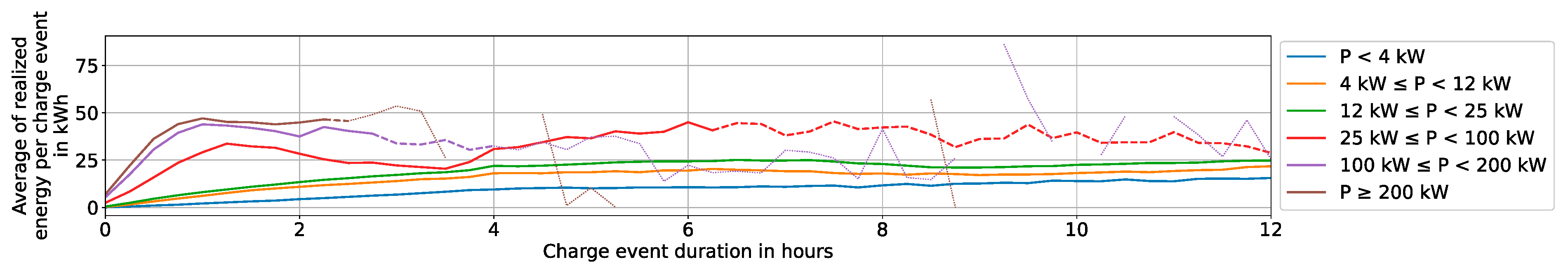
  • The EVSE’s power band is given using the upper and lower boundaries as shown in Figure 1. For instance, an EVSE with a rated power of 22 kW is part of the power band 12–25 kW.
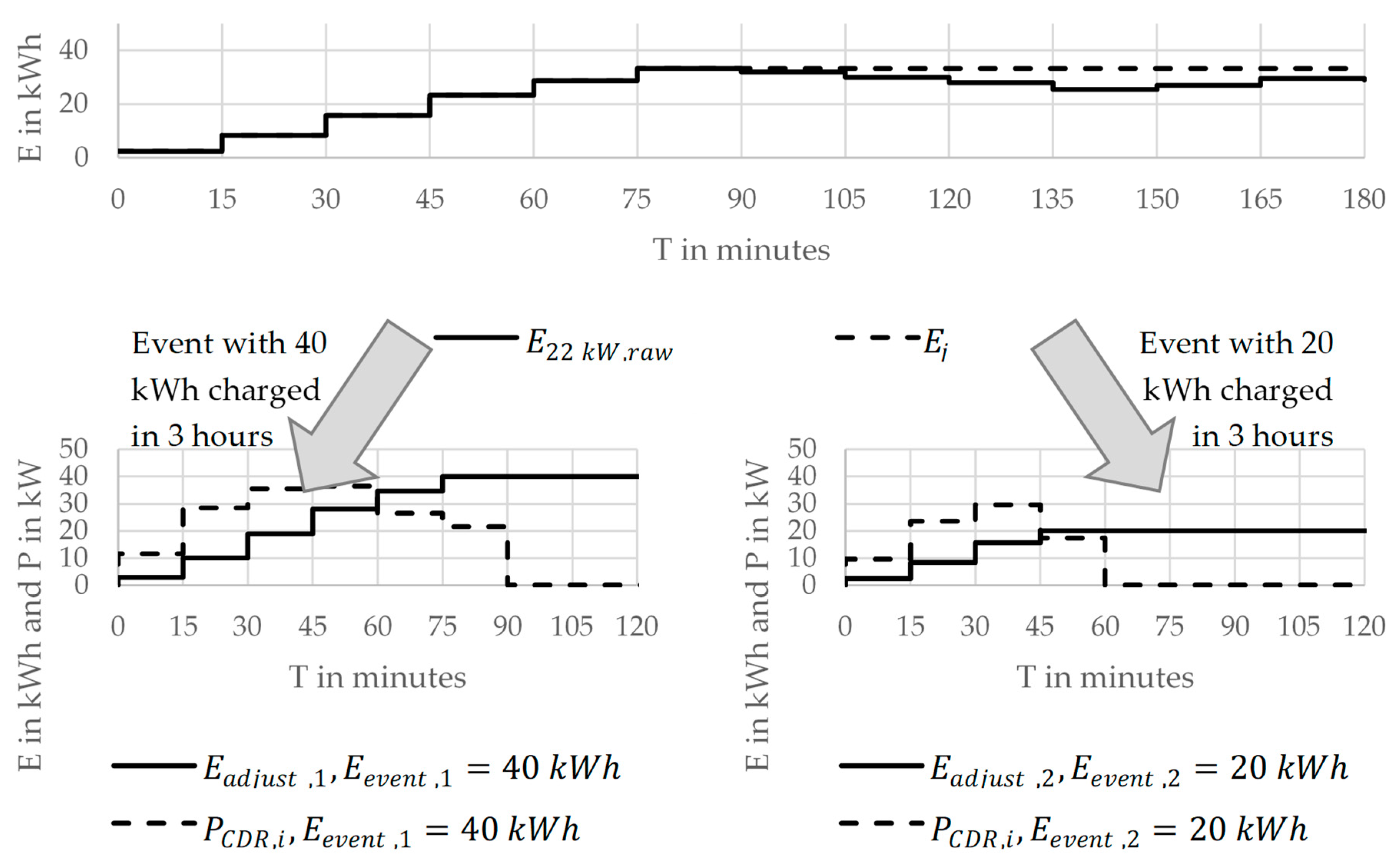
  • The selected curve of the consumed energy was transformed into a monotonously increasing curve by applying the cumulative maximum function defined as
    E j T = max E P i , r a w 0 , E P i , r a w T   w i t h   T 0 , T j
    where E P i , r a w T is the lookup function plotted in Figure 1 for the power level P i and the charge event duration T for the EVSE with index i , and E j T is the approximated energy curve for the charge event j . T is only defined in 0 , T j , where T j is the duration of the charge event j . The reason is that some charge events consumed less energy on average than the average of their shorter counterparts.
  • Next, we compared the energy that was consumed in the CDR under observation with the average amount of energy consumed in a charge event at an EVSE of the CDR’s power level. We also compare to the event duration to ensure that the energy transferred according to the modelled curve corresponded with the actual energy transfer.
    E a d j u s t , j T = E e v e n t , j i f   T > T j 0 e l i f   T < 0 0 T min ( P i , m E j τ d τ ) d τ e l i f   E j T j < E e v e n t , j min E j t ,   E e v e n t , j o t h e r w i s e
    where E e v e n t , j is the energy transferred in the charge event j as provided in the CDR data, m is a factor found numerically such that E a d j u s t , i , j T j = E e v e n t , j , and E a d j u s t , i , j t is the energy curve used to approximate the charge event over time. The third row of Equation (2) can be understood as linearly increasing the instantaneous power up to the EVSE’s limit if the average charge event would result in little energy transferred. The bottom part in turn can be understood as the car stopping charging once E j is reached.
  • The last step of the profile generation was to chain the various events into a singular time series per EVSE. To do so, the energy function was differentiated to obtain the power, which is summed up as
    P C D R , i t = t s t a r t , j t s t a r t s , i d E a d j u s t , j t t s t a r t , j d t
    where P C D R , i t is the instantaneous power at EVSE i based on the CDR records, and t s t a r t s , i is the set of all starting times in the form of date times at EVSE i .

2.2.4. Power Profiles for EVSEs without Full CDR Records

For the majority of EVSEs, particularly for fast-chargers, no complete CDR records are available. Instead, the start and stop times of charge events and their rated powers can be obtained. In other words, the charged energy for each charge event E e v e n t , j is unknown, which would fail the procedures described in the previous subsection.
The simplest approach to overcoming this issue is to assume that the transferred energy of each charging event corresponds to the definition of E j T in Equation (1) that is subsequently differentiated by
P a v e r a g e , i T = 0 i f   T < 0 d E j T d t E P i , r a w T E j T i f   0 T T j 0 o t h e r w i s e
In Equation (4), the term E P i , r a w T E j T   is used to scale the power curve, which is necessary as E j T may be larger than E P i , r a w T due to the maximum function used. This would lead to an overestimation of the power values and must be corrected.
The values underlying E P i , r a w T are the average values that may hide extreme values. To account for this, the flat and the peak estimation were developed. The flat estimation evenly spreads out the energy recharged during a charge event over time and is consequently a grid-friendly charging mode. The peak estimation charges at peak power until the energy according to E P i , r a w T are transferred and subsequently become 0. Both approaches are unrealistic and meant to define the two extremes between which the real usage lies. That is, the flat profile would require the exact knowledge of the duration of stay for an individual EV; the peak profile would require the vehicle to accept the rated power of the EVSE and to suddenly stop charging after a given energy transfer.
For an individual charge event, the flat power P f l a t , j , i is defined as
P f l a t , j , i T = 0 i f   T < 0 E P i , r a w T j T j i f   0 T T j 0 o t h e r w i s e
For the peak estimation, the charge event power P p e a k , j , i is defined as
P p e a k , j , i T = 0 i f   T < 0 P i i f   0 T E P i , r a w T j P i 0 o t h e r w i s e
The generation of a power profile for an EVSE from the power estimation is identical across all estimations, which is given as an example of the peak estimation by
P p e a k , i t = t s t a r t , j t s t a r t s , i P f l a t , j , i t t s t a r t , j

3. Results

This section provides the results obtained in this study. Section 3.1 starts with the results based on more detailed CDRs. Since full information of each PCS is available, the results can be used with high level of confidence. Section 3.2 augments these findings by showing the results for all PCSs with the availability data. This is particularly relevant for fast-chargers since only a very limited dataset is available for these chargers.

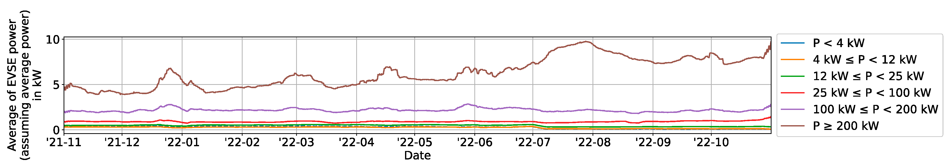
3.1. CDR-Based Results

This section introduces the results that can be obtained by analysing the CDRs. Section 3.1.1 begins by showing the shape of PCS utilisation across the power levels and area types for which sufficient data are available. Then, Section 3.1.2 provides the results on how the number of EVSEs per PCS affects utilisation.

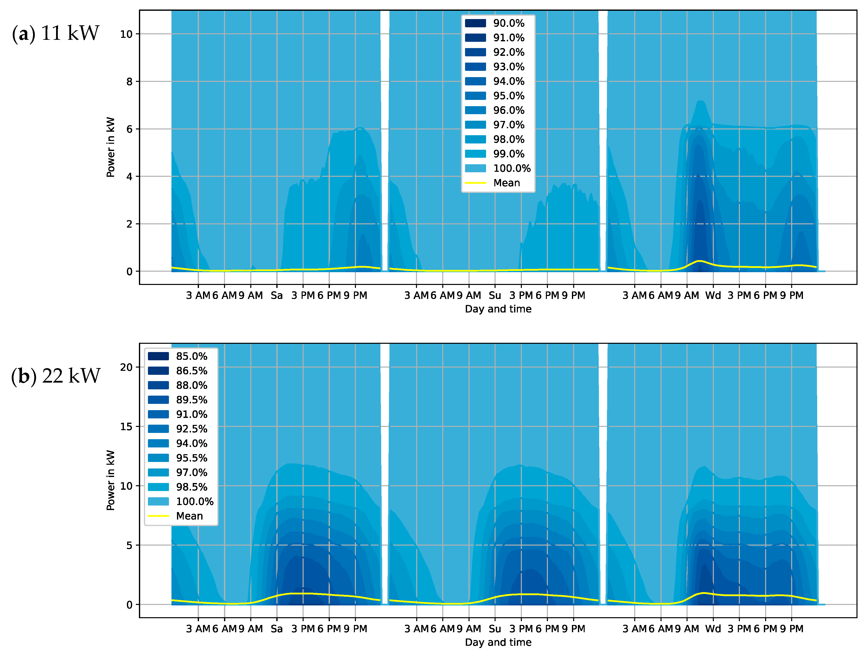
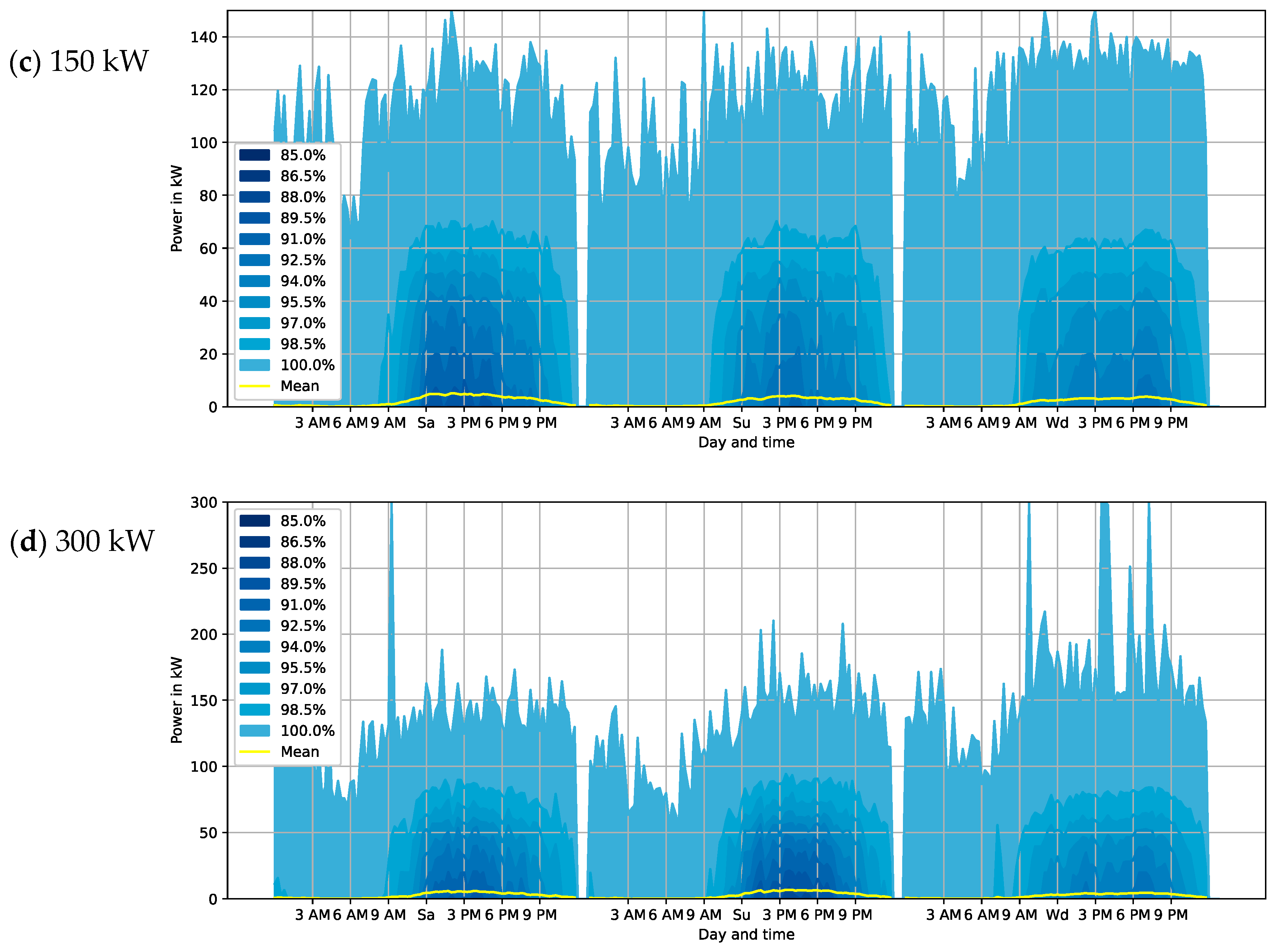
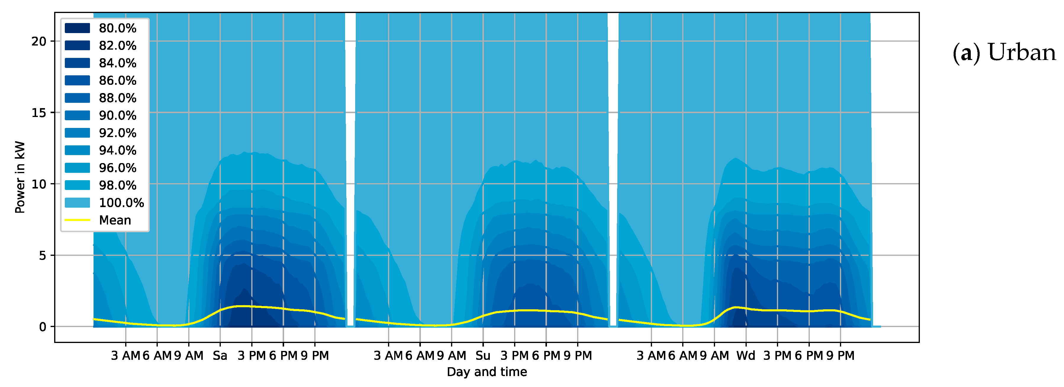
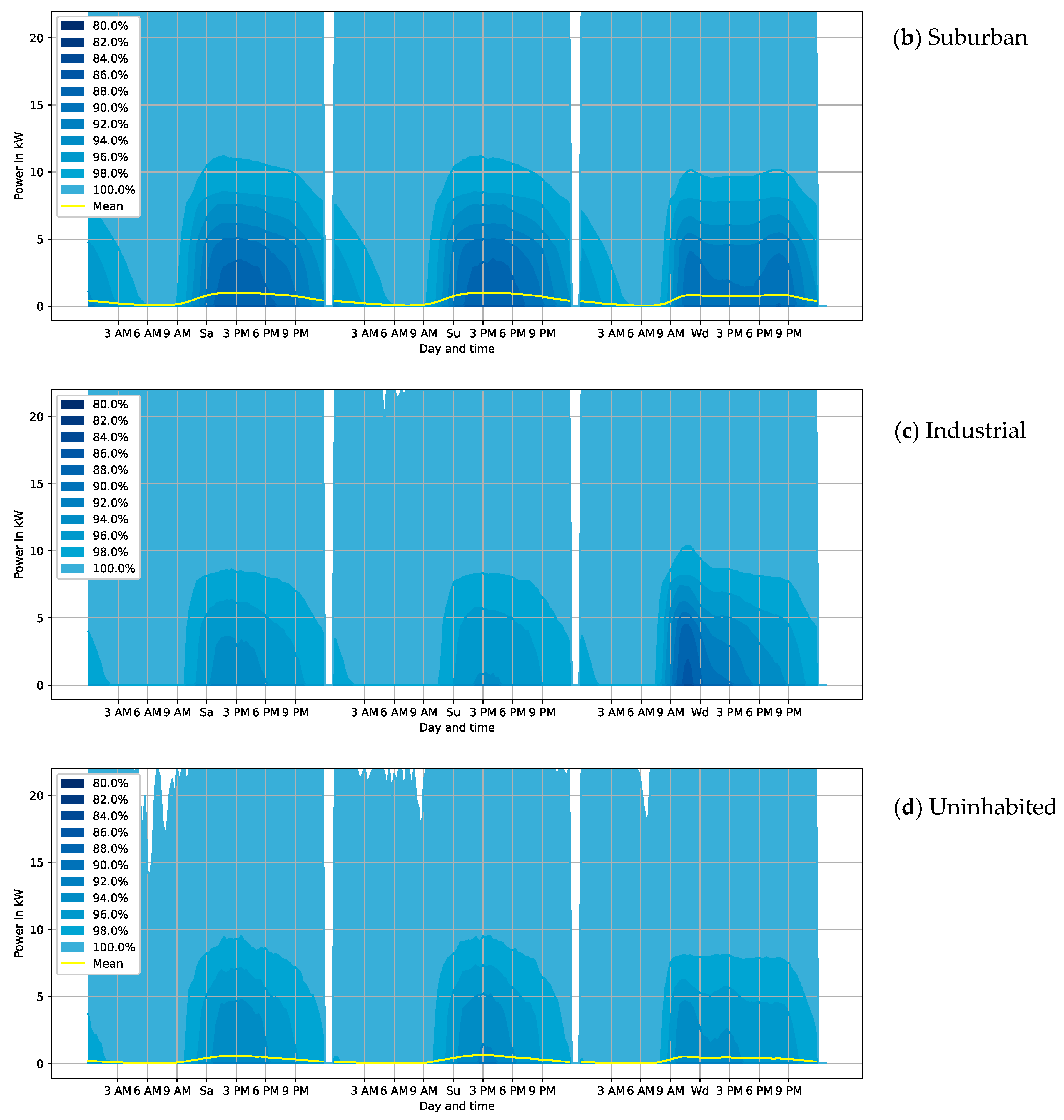
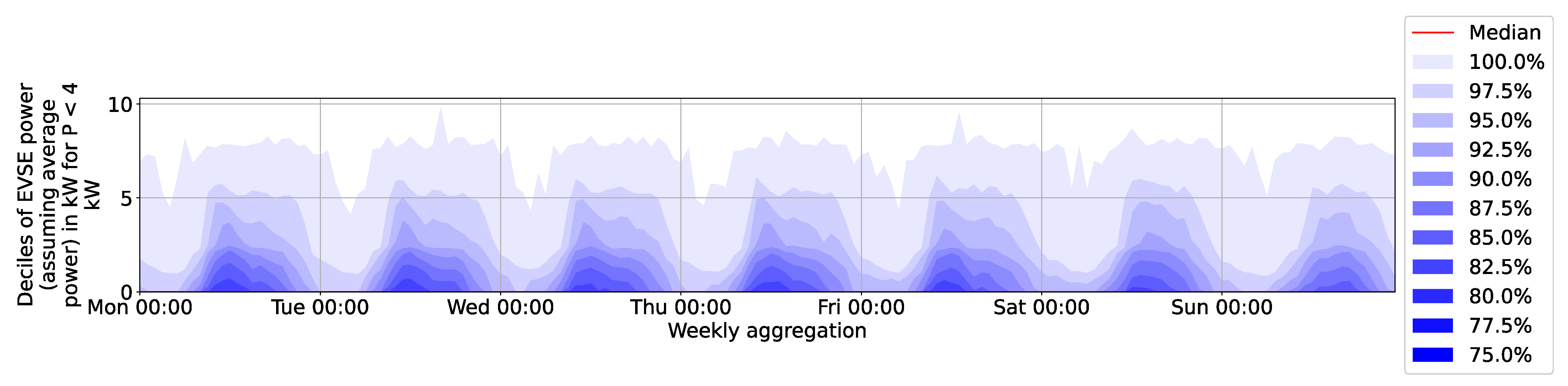
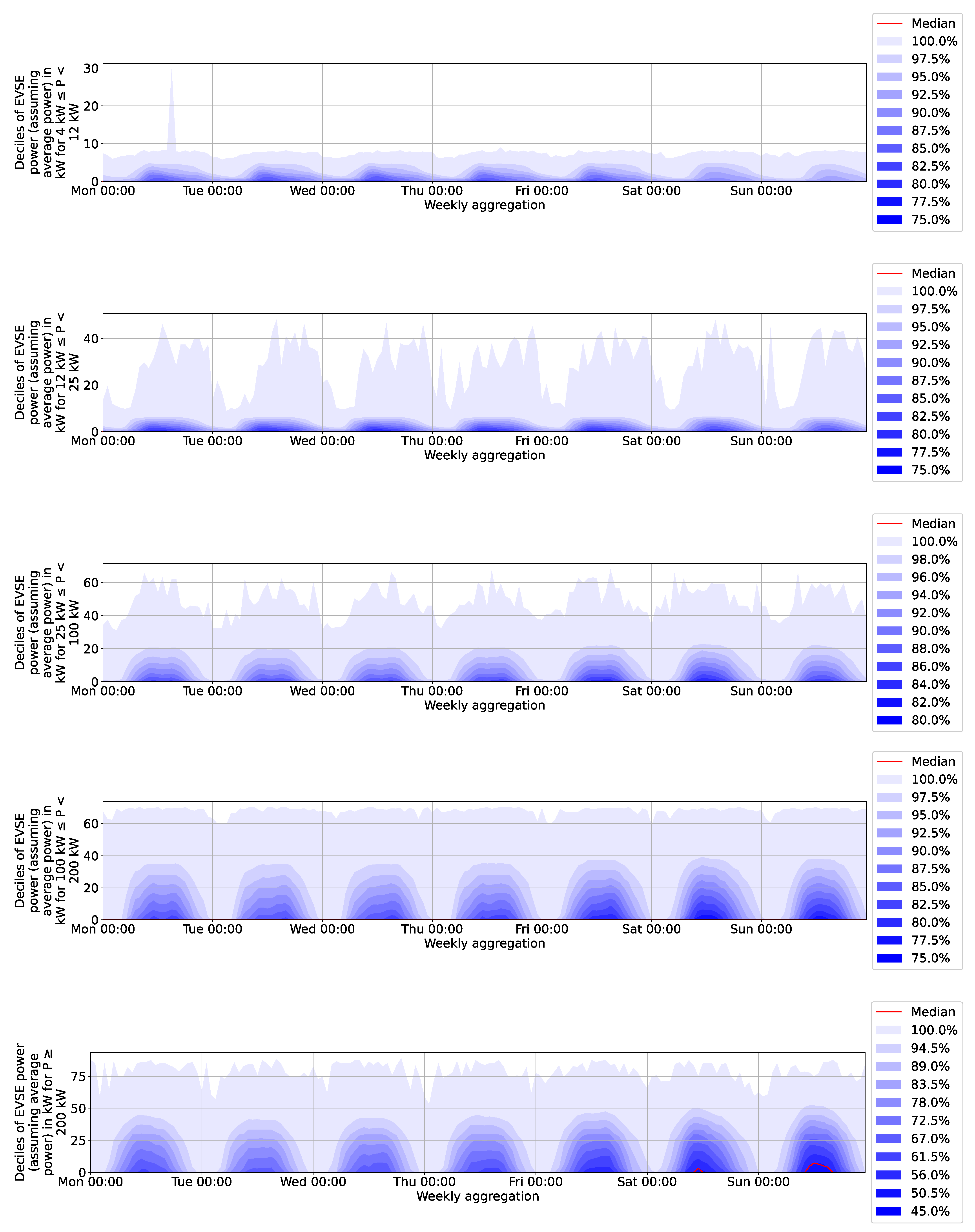
3.1.1. Weekly Profiles by Area Type and Power Level

Figure 3 shows the power flow at EVSEs across various area types and power levels for the day types of weekday (“Wd”), Saturday (“Sa”), and Sunday (“Su”). Note that public holidays were excluded from the analysis as there were too few in the observed period to make meaningful statements about them. From previous analysis [15,16], it appears plausible that public holidays can be reasonably represented as Sundays in terms of power demand profiles. Figure 4 extends the figure by focussing only on EVSEs with a rated power of 22 kW, but then splitting the data by area types.
Some observations can be made as follows: The power demand during the night is almost zero across all configurations shown in both figures and across all categories. The shape of the power flow during the day in turn differs significantly: Slower AC chargers, particularly the ones located in urban and suburban areas, experience two power peaks during weekdays. One occurs just before noon and can be explained by more charging processes starting over the course of the morning. The peak is before noon, since the bulk of charging processes starts at around 6 a.m. [16] and would have stopped by midday. The second peak occurs in the late evening and is the result of charging processes started after returning home. For EVSEs in industrial areas, only a single morning peak can be observed as few people live in such areas.
Additionally, it is found that the upper deciles are significantly higher than the average load per station. This indicates that the instantaneous power demand is much higher for certain stations and days. For the 22 kW EVSEs, the maximum instantaneous power demand is more than 20 times higher than the average power demand. This implies that the power grid supplying a single EVSE must be able to deliver the promised 22 kW; but as long as many are aggregated, the grid capacity can be much smaller than the sum of all installed capacity.
For fast-chargers, no singular spikes are observed. The power curve over the day follows a bell shape. Given the small number of fast-chargers for which we have a full CDR history (see Table 1), the reliability of this finding is limited and is expanded in the results based solely on availability data as shown in Section 3.2.

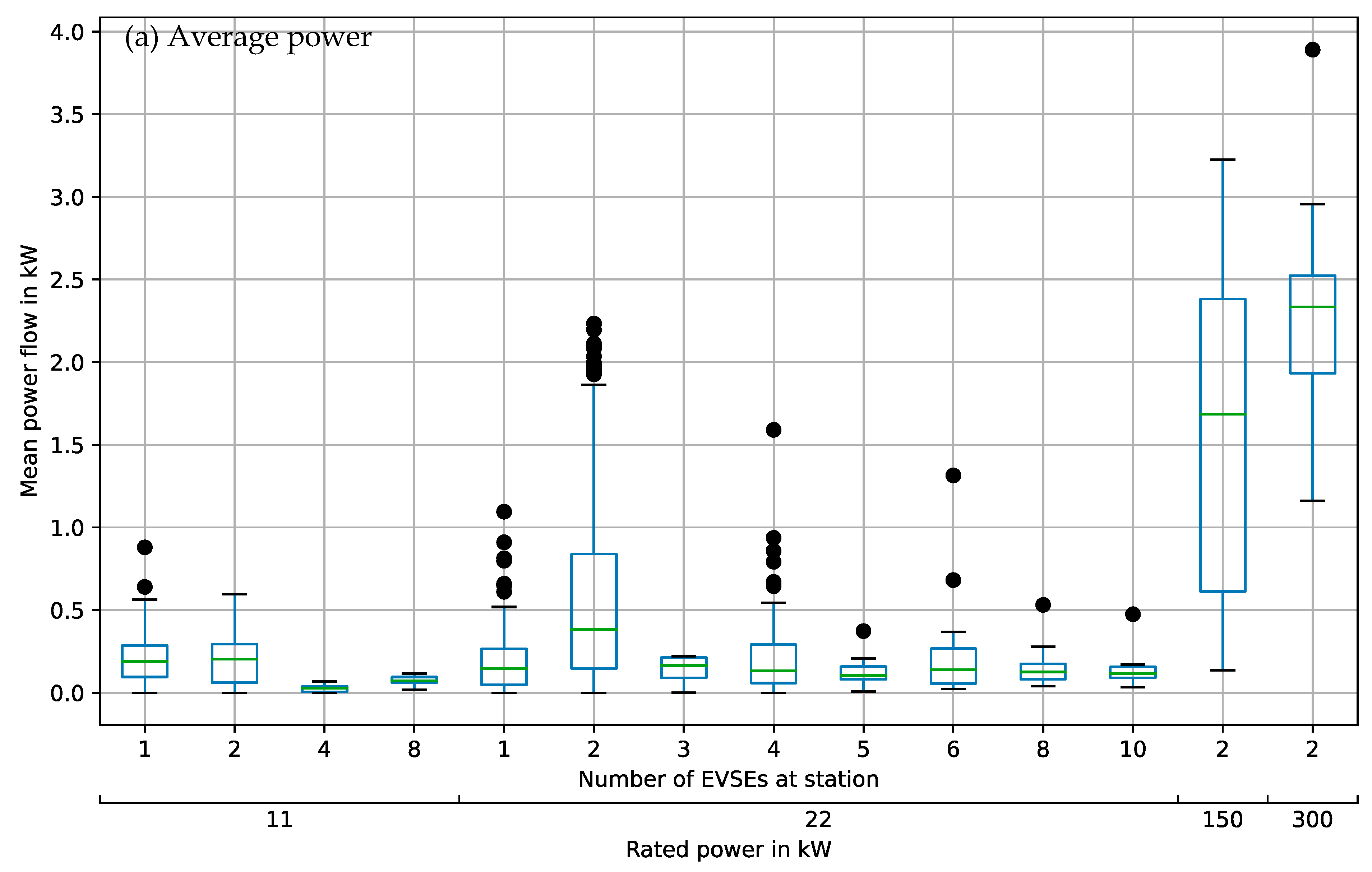
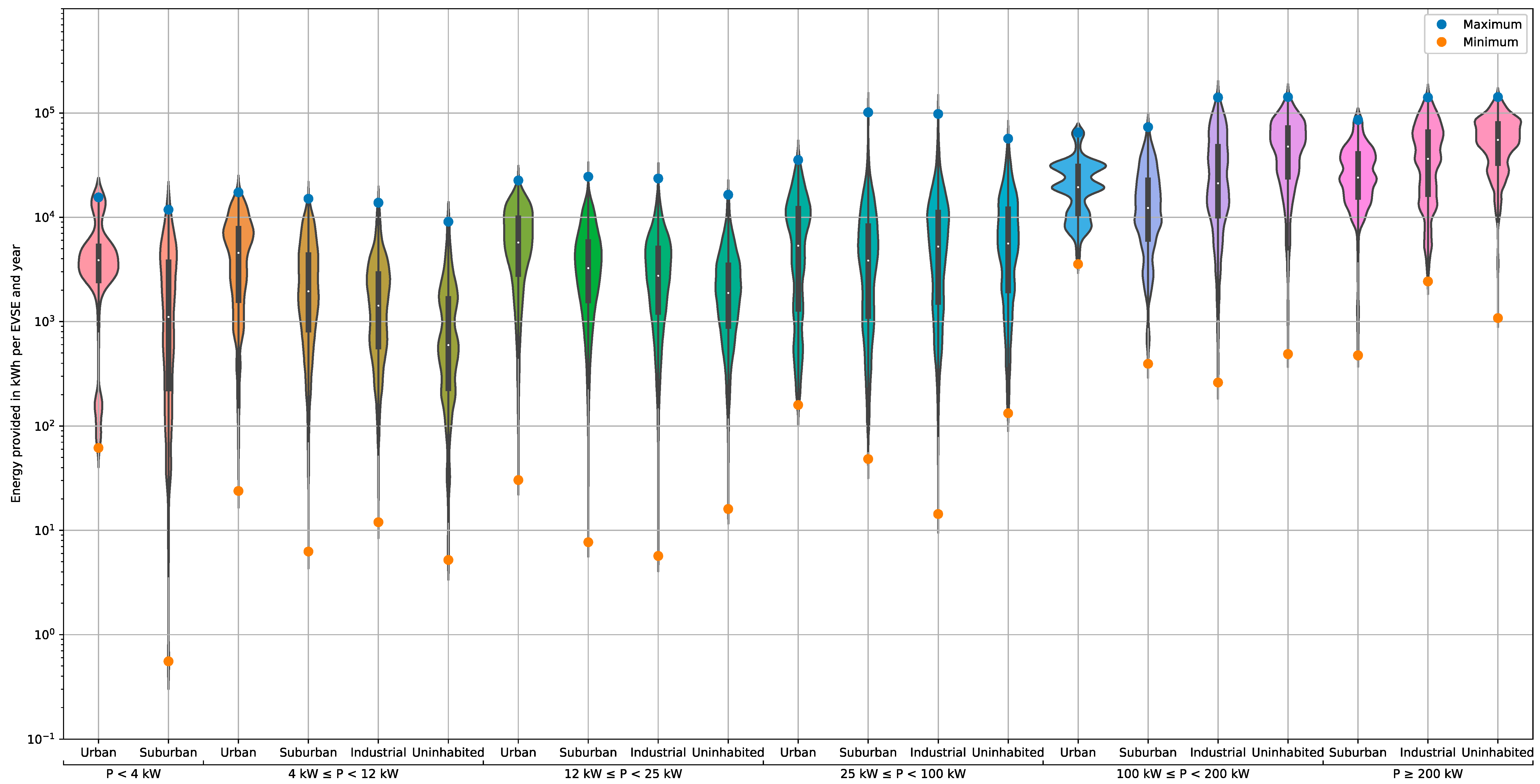
3.1.2. Comparison of Different Numbers of EVSEs per PCS

One question surrounding the construction of PCSs is whether it is sensible to invest in the relatively expensive curbside chargers, often with two or four EVSEs, or to invest in larger car parking locations. Small installations with only two EVSEs tend to be highly accessible and visible since they are typically located directly on the curbside. Larger installations, however, are usually located in (multi-storey) car parks. These are typically less visible and it therefore appears reasonable to assume that their utilisation would be lower than their smaller counterparts. Figure 5 provides the results on this issue by showing the mean (top) and maximum (bottom) power flow per EVSE for the power levels and the number of EVSEs whereby at least five PCSs were part of our dataset.
For the AC PCSs with a rated power of either 11 or 22 kW per EVSE, a trend is visible: PCSs with only two EVSEs experience the highest average power flow and the median power flow decreases with every EVSE added to the PCSs. This trend stops being significant if the PCS hosts eight or more EVSEs. A second aspect to note is that the mean power flow rises with the rated power. However, the maximum power flow per EVSE does not decrease at the same speed. This means that, at least in the relatively naïve charging approach chosen for this study, grid costs do not decrease significantly with scale. However, it can be reasonably assumed that an intelligent load management system may decrease grid costs as long as the information regarding the duration of stay of users is available.

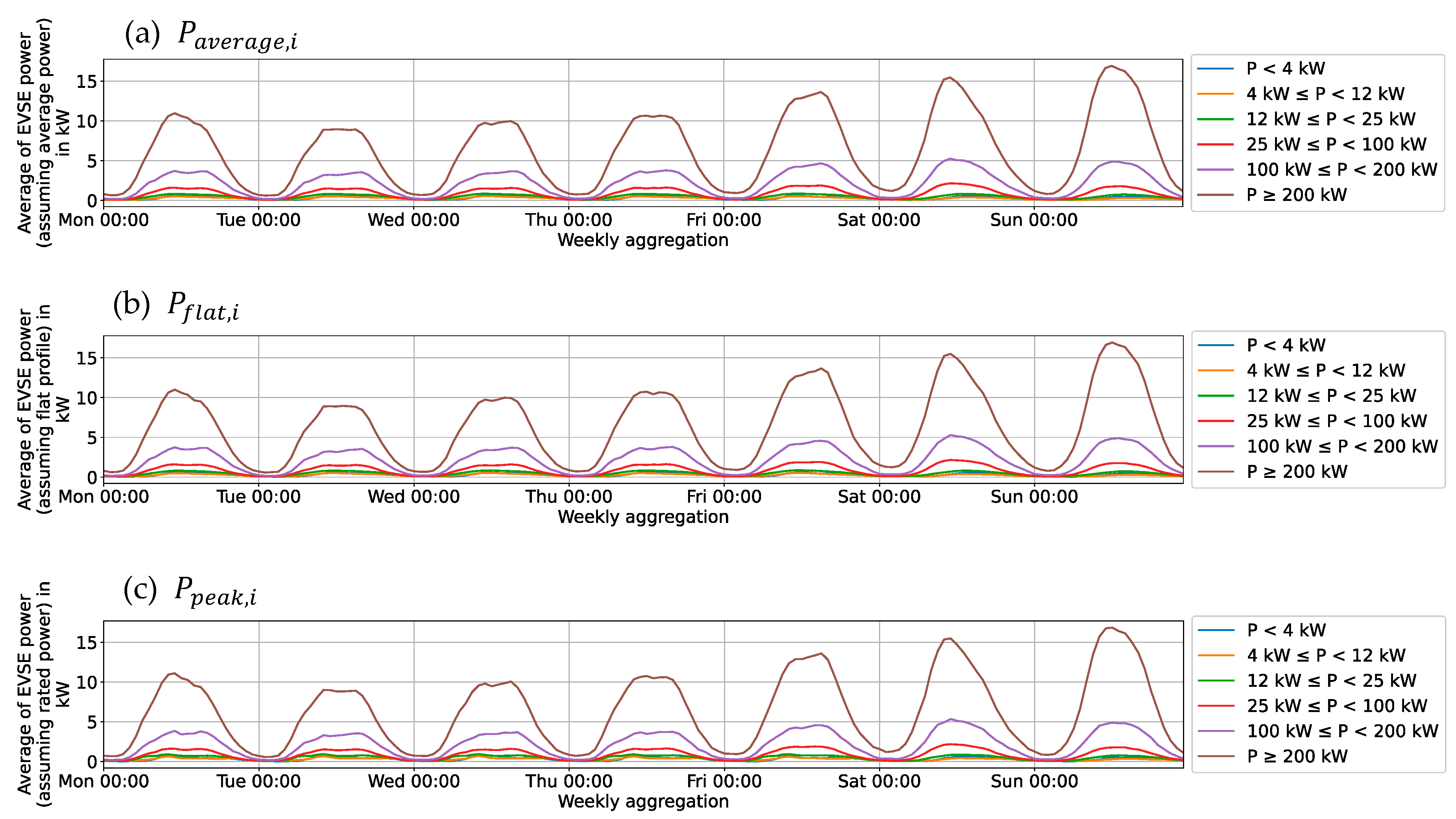
3.2. Results Based on Availability Data

A full CDR record was only available for a small number of EVSEs and those were predominantly slower AC chargers. The following results complete this picture by showing the results for a much larger dataset of EVSEs for which availability data are present in our dataset. Given that these results are similar in structure to our previous publication [16], we use the formatting of this presentation in an effort to ensure comparability.
Figure 6 shows the results of this analysis by displaying the profiles over the course of the week that could be generated using the methodology introduced in Section 2.2.4.
Analysing the three profiles carefully, it can be observed that the profiles generated from P a v e r a g e , i and P p e a k , i are reasonably close to the profiles generated using CDRs, especially for the slower AC EVSEs. For fast-chargers, the number of EVSEs for which a full CDR history is available is insufficient to make the same claim with the same level of confidence, but the results are reasonably close. Figure 6 does show slightly higher values than Figure 3. An explanation for this could be that half of the data used to define E P i , r a w are roaming events (“Roaming” refers to customers of an e-mobility service provider (EMP) charging at the PCS of a CPO that is not part of the same company. Usually, platform operators such as Hubject and e-clearing have contracts with many EMPs and CPOs to enable such transactions. This typically happens when people are travelling to other cities and cannot access the PCSs of their home CPO) with the share being even higher for EVSEs with a high rated power. It is reasonable to assume that energy consumption while roaming is higher than the consumption if one charges at other EVSEs, since roaming typically happens when one is driving longer distances. This explains the deviation in the maximum of the two approaches.
Focussing on fast-chargers, it is clear that the shape of the power demand closely follows the occupation shape in Figure 9 in [15], which can be explained by the few and short idle times at fast-chargers. The short idle times also mean that the three approaches to defining the power level shown in Section 2.2.4 create almost identical results for the average power flow. The situation changes if one looks at the maximum power flows, which are necessarily much higher in the P p e a k , i scenario.
Since Figure 6 only shows average values, the decimal plots analogous to Figure 3 in Appendix A are shown in Figure A1. Since the peak values are largely determined by the estimation function, these maximum values should be used with discretion.
Travel patterns and consequent power profiles are not uniform over the year. Figure 7 shows the non-aggregated and smoothed power profile for the timespan analysed in this study. For the fast-chargers with a rated power above 200 kW, clear consumption peaks can be observed. The average power rises toward the end of 2021, in March, the end of May, and early June, July until early August, and again at the end of September. All of these periods are vacation periods in Germany during which people often take longer-distance trips and fast-charging is required. The only exception is the end of May and early June when there are no vacations, but many public holidays are either on Thursdays or on Mondays. These long weekends are also typically used for long-distance travelling. The results also show that charging stations are predominantly occupied on weekends, which is again a time when people tend to travel more. Note that the small increases in power consumption toward the end of the observed timeframe are an artefact of data processing: as EVSEs are only observed between the first and last status change, the number of EVSEs under observation reduces toward the end of the timeframe. This causes the share of EVSEs occupied to be larger as generally more EVSEs drop out at the two ends that are available rather than occupied.
Figure 8 augments the previous analysis by showing how much energy various EVSEs provide depending on their power levels and whereabouts. Note that the plot is made with a logarithmic scale, and it is quite clear that there are major differences between various EVSEs.
For conventional 22 kW chargers, the top-performing EVSE in an urban setting was able to supply 25 MWh, which corresponds to an annual average power flow of 2.9 kW. The vast majority, however, only supply about 300 kWh per year which is less than a thirtieth of the top performer. For fast-chargers, the difference is not that large and the top performer only sells about twice as much energy as the bulk of the EVSEs.

4. Discussion and Conclusions

The results of this study show how the power demand of PCSs in Germany is shaped for several types of days in a week. Given the large underlying dataset, it can be assumed that this behaviour is reasonably representative of the studied period (1 November 2021–31 October2022). Individual PCSs may show different behaviours, depending on local circumstances. The estimations of P a v e r a g e , i and P p e a k , i for PCSs, for which only the availability data are accessible, show strong resemblance with the CDR-based data and can therefore be assumed to be a reasonable approach.
From an infrastructure point of view, the observed power profile at AC chargers is not ideal as it coincides with other times when the distribution grid is already heavily loaded, such as in the early evening hours for urban and suburban areas. In industrial areas, high power peaks in mornings may be problematic as this coincides with the times when factories and businesses would launch their operations and consequently reach high-power demands.
A positive aspect is that the load profiles of fast-chargers and of chargers located in urban areas coincide very well with a typical PV generation profile, making the coupling of charging infrastructure with these renewable generators attractive. A detailed discussion on this issue is beyond the scope of this study, but a calculation of the goodness of fit between a PV generation curve and the power demand curves can be found in Appendix B. This could be achieved by covering parking lots with PV panels as this keeps vehicles cool—thus reducing battery ageing—and generates electricity at the right location.
Given that many fast-chargers are equipped with high grid connection capacities and are frequently located along highways and other locations with low population density, a coupling with large renewable generators seems highly attractive. The fact that both PV generation and power consumption at PCSs are intermittent makes it attractive to install a buffer energy storage as this combination could be used to significantly reduce the required grid capacity.
Some limitations have to be considered when working with these results. First, the CDR-based results are primarily valid for EVSEs rated at 22 kW. For other power levels, the number of EVSEs observed is smaller leading to reduced representativeness and reliability of the results. The potential systematic biases have been introduced in the data section and readers are encouraged to carefully study these before applying the found results. For the results based on the availability data, it has to be kept in mind that especially for fast-chargers, the power curves used are primarily based on roaming events. It seems plausible from our results that this introduces a small systematic error since roaming events could generally be assumed to have a higher energy throughput than their non-roaming counterparts. Even given this slight limitation, it is highly probably that this effect only influences the amplitude of the curve rather than its shape. Given that the error is upwards and small, it appears reasonable for a grid operator to plan with the shown curves as this would result in only a minimal oversizing of hardware. For energy purchasing, readers should compare the energy throughput shown with their individual energy throughputs, as these should be readily available in any company.
A third limitation is that the charging patterns have undergone a highly dynamic evolution over past years and it seems highly likely that this will continue to be the case. More vehicles sharing a single EVSE, higher charging powers, a more diverse user base, and many other factors would contribute to changing utilisation patterns. As Figure 7 shows, small changes especially for higher power levels are already visible within the one-year period. Unfortunately, it is not possible to differentiate between seasonal effects and effects due to the continuously changing market as doing so would require a steady-state situation as a reference. Determining the exact shape and influence of the long-term changes on the load profiles is beyond the scope of this study as the data-driven approaches such as those used in this paper can only represent the present and past. Interested readers should therefore check whether the overall patterns shown are still valid and may adjust the curves’ amplitude according to their observations and assumptions. Some guidance may be obtained from tools such as the StandortTOOL [25] or model-based approaches [7,10]. Some trends that may be hypothesised are that more vehicles per EVSE will result in a higher average loading and a flatter loading curve. With increasing battery capacity per vehicle, it also appears probable that average charging powers at fast-charging stations will rise in future.
When properly addressing the mentioned limitations, the found patterns and derived conclusions aid readers from academia, industry, politics, and other organisations in their understanding and improvement of PCS usage due to the broad and representative dataset used.

Supplementary Materials

The following supporting information can be downloaded at: https://www.mdpi.com/article/10.3390/en16062619/s1.

Author Contributions

Conceptualisation, C.H. and J.F.; methodology, C.H.; software, C.H.; validation, C.H. and J.F.; formal analysis, C.H.; investigation, C.H.; resources, C.H. and D.U.S.; data curation, C.H.; writing—original draft preparation, C.H., L.Z. and X.L.; writing—review and editing, J.F. and D.U.S.; visualisation, C.H.; supervision, J.F. and D.U.S.; project administration, C.H., J.F. and D.U.S.; funding acquisition, C.H., J.F. and D.U.S. All authors have read and agreed to the published version of the manuscript.

Funding

This research was funded by the Federal Ministry for Economic Affairs and Climate Action (BMWK) on the basis of a decision by the German Bundestag, grant number 01MV20001A. The APC was funded by institute funds. This study is in part supported by the Ministry of Science and Technology of the People’s Republic of China under grant 2022YFE0103000.

Data Availability Statement

The numerical results of all figures shown in this paper can be found in the appended dataset linked in the Supplementary Materials section. Note that for some decile plots, the differences between the decile levels are given.

Acknowledgments

The work shown in this paper relies upon the datasets provided to us by our industry partners SMART/LAB and Hubject in the context of the project “BeNutz LaSA” [22]. We are grateful for the data provision as well as for fruitful discussions about the contents of this work.

Conflicts of Interest

The authors declare no conflict of interest.

Appendix A. Decile Plots Created with Availability Data

Figure A1 shows the decile plots that were generated using the power profile estimation for EVSEs; no CDR record was available using the P a v e r a g e , i estimation. Note that the values shown may exceed the rated station limit if many events were started at the same EVSE within a short period or due to rounding errors.
Figure A1. Analogous plots to Figure 3 using the P a v e r a g e , i estimation for the various power levels defined in [16]. Note that the median is on the zero-line in all visualisations except for the last.
Energies 16 02619 g0a1aEnergies 16 02619 g0a1b

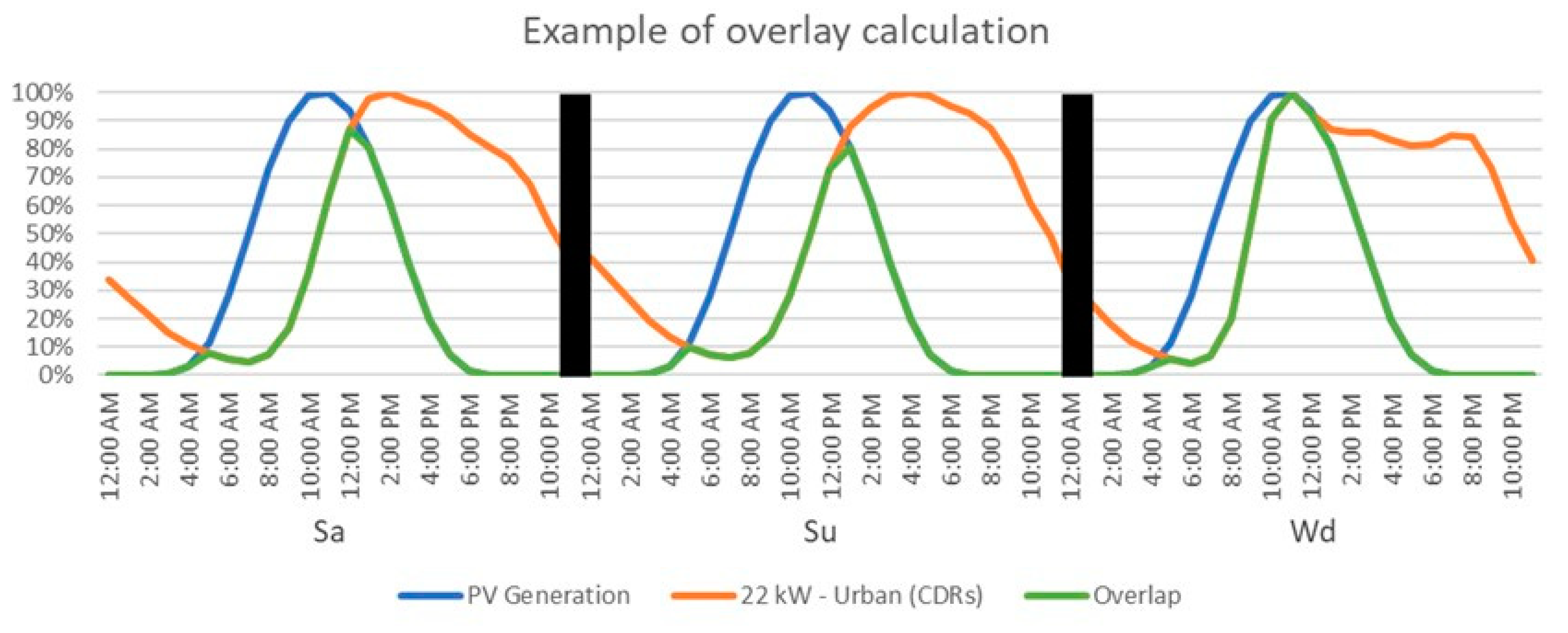
Appendix B. Overlap of PV Generation and Charging Demand

The power curves of the charging stations visually appear to have a strong overlap with PV generation curves. This intuition can be verified by comparing the PV generation curve of Germany retrieved from [26] with the mean power demand curves found in Figure 4 and Figure 6 (using the P a v e r a g e approach as an example). Since PV generation can be scaled freely, we normalised all of the curves by the maximum of the curve per day type. After doing so, we determined the following values for each day type and power demand curve. The calculation was based on the CDR-derived curves outlined in Section 2.2.3, but the same concept may be applied to the curve definitions given in Section 2.2.4.
O v e r l a p d t , a t = 0 24 h min P V d t t ¯ , P C D R , d t , a t t ¯ d t
E x c e s s P V , d t , a t = 0 24 h P V d t t ¯ min P V d t t ¯ , P C D R , d t , a t t ¯ d t
E x c e s s d e m a n d , d t , a t = 0 24 h P C D R , d t t ¯ min P V d t t ¯ , P C D R , d t , a t t ¯ d t
where P V d t t ¯ is the average PV generation for a day type d t in the period studied in this paper and P C D R , d t , a t t ¯ is the average power curve generated in this paper for a specific day type and area type a t . The procedure is visualised for the example of a power curve in urban areas at 22 kW chargers in Figure A2.
Figure A2. Example of the overlay calculation using the mean power curve for 22 kW EVSEs in an urban setting from Figure 4a. Generation and consumption lines are scaled such that the peak value for each day type is one. The area under the green curve is the overlapping area and the areas between the blue and green and the orange and green lines are excess generation and consumption, respectively.
Energies 16 02619 g0a2
From these three values, a goodness of fit G O F can then be derived by comparing the various integrals as follows. Table A1 shows the results of this computation for the data shown in Figure 4 and Figure 6a. Note that the derived G O F is different from the typically used metrics of self-consumption and self-sufficiency. These two metrics can only be calculated for generation and consumption curves where the absolute magnitude is known since an excessively large PV plant will result in a high degree of self-sufficiency and a low degree of self-consumption. A negligibly small PV plant will result in the reverse, independent of the goodness of fit. Given that PV plants can be scaled independently, the two traditional metrics cannot be employed.
G O F d t , a t = O v e r l a p d t , a t O v e r l a p d t , a t + E x c e s s P V , d t , a t + E x c e s s d e m a n d , d t , a t
Table A1. G O F for the mean power curves shown in Figure 4 and Figure 6a. Green indicates high values and red indicates low values.
SaSuWd
Based on
Figure 4
22 kW—Urban0.2860.2520.394
23 kW—Suburban0.2870.2740.371
22 kW—Industrial0.3170.2750.533
22 kW—Uninhabited0.2990.3020.451
Based on
Figure 6a
P < 4 kW0.3450.3290.481
4 kW ≤ P < 12 kW0.3840.3450.501
12 kW ≤ P < 25 kW0.4480.4190.519
25 kW ≤ P < 100 kW0.6100.5340.564
100 kW ≤ P < 200 kW0.6070.5490.546
P ≥ 200 kW0.6540.5850.571

Appendix C. Matching Table for the Corine Land Cover Model Categories

Table A2 shows the matching table used for this paper that was originally published as a part of [15].
Table A2. Matching table used to determine the category used in this paper from the more fine-grained categories available in the Corine land cover model.
Corine CategoriesCategory Used
Continuous urban fabricUrban
Discontinuous urban fabric, green urban areas, sport and leisure facilitiesSuburban
Industrial or commercial units, port areas, airports, mineral extraction sites, construction sitesIndustrial
Road and rail networks and associated land, port areas, airports, mineral extraction sites, dump sites, construction sites, green urban areas, sport and leisure facilities, non-irrigated arable land, vineyards, fruit trees and berry plantations, pastures, complex cultivation patterns, land principally occupied by agriculture, with significant areas of natural vegetation, broad-leaved forest, coniferous forest, mixed forest, natural grasslands, moors and heathland, transitional woodland–shrub, beaches, dunes, sands, inland marshes, peat bogsUninhabited
Dump sites, construction sites, green urban areas, sport and leisure facilities, non-irrigated arable land, vineyards, fruit trees and berry plantations, pastures, complex cultivation patterns, land principally occupied by agriculture, with significant areas of natural vegetation, broad-leaved forest, coniferous forest, mixed forest, natural grasslands, moors and heathland, transitional woodland–shrub, beaches, dunes, sands, inland marshes, peat bogs, water courses, water bodies, estuaries, sea and oceanNon-fitting

References

  1. Hu, X.; Yuan, H.; Zou, C.; Li, Z.; Zhang, L. Co-estimation of state of charge and state of health for lithium-ion batteries based on fractional-order calculus. IEEE Trans. Veh. Technol. 2018, 67, 10319–10329. [Google Scholar] [CrossRef]
  2. Li, X.; Wang, Z.; Zhang, L.; Sun, F.; Cui, D.; Hecht, C.; Figgener, J.; Sauer, D.U. Electric vehicle behavior modeling and applications in vehicle-grid integration: An overview. Energy 2023, 268, 126647. [Google Scholar] [CrossRef]
  3. Shell Recharge Solutions. “EV Driver Survey Report 2022”, Shell Recharge Solutions [Online]. 2022. EV Driver Survey Report. 2022. Available online: https://shellrecharge.com/en-gb/solutions/knowledge-centre/reports-and-case-studies/ev-driver-survey-report (accessed on 27 June 2022).
  4. Bibra, E.M.; Connelly, E.; Dhir, S.; Drtil, M.; Henriot, P.; Hwang, I.; Le Marois, J.B.; McBain, S.; Paoli, L.; Teter, J. Global EV Outlook 2022. International Energy Agency, Paris. Available online: https://www.iea.org/reports/global-ev-outlook-2022 (accessed on 29 August 2022).
  5. BDEW. Standardlastprofile Strom. Available online: https://www.bdew.de/energie/standardlastprofile-strom/ (accessed on 11 December 2022).
  6. Bollerslev, J.; Andersen, P.B.; Jensen, T.V.; Marinelli, M.; Thingvad, A.; Calearo, L.; Weckesser, T. Coincidence factors for domestic ev charging from driving and plug-in behavior. IEEE Trans. Transp. Electrific. 2022, 8, 808–819. [Google Scholar] [CrossRef]
  7. Held, L.; Märtz, A.; Krohn, D.; Wirth, J.; Zimmerlin, M.; Suriyah, M.R.; Leibfried, T.; Jochem, P.; Fichtner, W. The influence of electric vehicle charging on low voltage grids with characteristics typical for germany. WEVJ 2019, 10, 88. [Google Scholar] [CrossRef] [Green Version]
  8. Mitrakoudis, S.G.; Alexiadis, M.C. Modelling electric vehicle charge demand: Implementation for the greek power system. WEVJ 2022, 13, 115. [Google Scholar] [CrossRef]
  9. Celli, G.; Soma, G.G.; Pilo, F.; Lacu, F.; Mocci, S.; Natale, N. Aggregated electric vehicles load profiles with fast charging stations. In Proceedings of the 2014 Power Systems Computation Conference, Wrocław, Poland, 18–22 August 2014; pp. 1–7. [Google Scholar]
  10. Islam, M.S.; Mithulananthan, N. Daily EV load profile of an EV charging station at business premises. In Proceedings of the 2016 IEEE Innovative Smart Grid Technologies–Asia (ISGT-Asia), Melbourne, Australia, 28 November–1 December 2016; pp. 787–792. [Google Scholar]
  11. Hu, Q.; Li, H.; Bu, S. The prediction of electric vehicles load profiles considering stochastic charging and discharging behavior and their impact assessment on a real uk distribution network. Energy Procedia 2019, 158, 6458–6465. [Google Scholar] [CrossRef]
  12. Flammini, M.G.; Prettico, G.; Julea, A.; Fulli, G.; Mazza, A.; Chicco, G. Statistical characterisation of the real transaction data gathered from electric vehicle charging stations. Electr. Power Syst. Res. 2019, 166, 136–150. [Google Scholar] [CrossRef]
  13. Hecht, C.; Figgener, J.; Sauer, D.U. Simultaneity factors of public electric vehicle charging stations based on real-world occupation data. WEVJ 2022, 13, 129. [Google Scholar] [CrossRef]
  14. Uimonen, S.; Lehtonen, M. Simulation of electric vehicle charging stations load profiles in office buildings based on occupancy data. Energies 2020, 13, 5700. [Google Scholar] [CrossRef]
  15. De Santis, M.; Federici, L. Preliminary study on vehicle-to-grid technology for microgrid frequency regulation. SAE Tech. Pap. Ser. 2022, 24, 19. [Google Scholar]
  16. Hecht, C.; Das, S.; Bussar, C.; Sauer, D.U. Representative, empirical, real-world charging station usage characteristics and data in Germany. Etransportation 2020, 6, 100079. [Google Scholar] [CrossRef]
  17. Hecht, C.; Figgener, J.; Sauer, D.U. Analysis of electric vehicle charging station usage and profitability in germany based on empirical data. Iscience 2022, 25, 105634. [Google Scholar] [CrossRef] [PubMed]
  18. Wolbertus, R.; Kroesen, M.; van den Hoed, R.; Chorus, C. Fully charged an empirical study into the factors that influence connection times at EV-charging stations. Energy Policy 2018, 123, 1–7. [Google Scholar] [CrossRef] [Green Version]
  19. Hecht, C.; Spreuer, K.G.; Figgener, J.; Sauer, D.U. Market review and technical properties of electric vehicles in germany. Vehicles 2022, 4, 903–916. [Google Scholar] [CrossRef]
  20. Statistisches Bundesamt Deutschland. Experimentelle Daten–Mobilitätsindikatoren mit Mobilfunkdaten. Available online: https://www.destatis.de/DE/Service/EXDAT/Datensaetze/mobilitaetsindikatoren-mobilfunkdaten.html (accessed on 27 January 2022).
  21. SMART/LAB. SMART/LAB–Hier Entsteht die Zukunft der Elektromobilität. Available online: https://smartlab-gmbh.com/ (accessed on 28 December 2022).
  22. Hecht, C. BeNutz LaSA: Bessere Nutzung von Ladeinfrastruktur Durch Smarte Anreizsysteme. Available online: https://benutzlasa.de/ (accessed on 19 March 2021).
  23. Hubject, Hubject | The World’s Largest International eRoaming Network. Available online: https://www.hubject.com/ (accessed on 28 December 2022).
  24. EEA. Corine Land Cover (CLC) 2018, Version 2020_20u1. Brussels: European Environment Agency (EEA) under the Framework of the Copernicus Programme. 2018. Available online: https://land.copernicus.eu/pan-european/corine-land-cover/clc2018 (accessed on 24 January 2020).
  25. Bundesministerium für Digitales und Verkehr, NOW GmbH, and Nationale Leitstelle Ladeinfrastruktur, StandortTOOL. Available online: https://www.standorttool.de/ (accessed on 9 February 2023).
  26. Fraunhofer ISE, Gesamte Nettostromerzeugung in Deutschland. [Online]. Available online: https://www.energy-charts.info/charts/power/chart.htm?l=de&c=DE&legendItems=000000000000000010000&year=2021&interval=year&download-format=text%2Fcsv&source=total (accessed on 10 February 2023).
Figure 1. Energy consumed by charge event duration and charging station power level. Example of how to read it: if a charge event occurs at an EVSE with a rated power between 12 and 25 kW and lasts 4 h, a sum energy of 22 kWh would be probably consumed. The data shown are similar to that in Figure 5 in [16], but with the time range used in this study.
Energies 16 02619 g001
Figure 2. An example of the power curve generation process for two charging events lasting 180 min at a station with the rated power of P i = 22   kW . The event with index j = 1 (bottom left) sees an energy transfer of E e v e n t , 1 = 40   kWh and is above the raw energy curve. The event with index j = 2 (bottom right) sees an energy transfer of E e v e n t , 2 = 20   kWh that is below the original energy transfer. Note that the curves E 22   k W , r a w , E j , and E a d j u s t , 2 ,   E e v e n t , 2 initially overlap.
Energies 16 02619 g002
Figure 3. Distribution (area plot) and mean (line) of EVSE power flow by day type and time of day. The y-axis is limited to the EVSEs’ installed power. When working with the curves, keep the constituting area types for each power level shown in Table 1 in mind, particularly with a view on EVSEs with a rated power of 11 kW. Percentage values in the legend describe the share of points that lie beneath the indicated line. Example of how to read it: on a Saturday at noon, 95.5% of EVSEs with a rated power of 22 kW see a power flow of 7.71 kW or less.
Energies 16 02619 g003aEnergies 16 02619 g003b
Figure 4. Distribution (area plot) and mean (line) of EVSE power flow by day type and time of day for EVSEs with a rated power of 22 kW. The y-axis was capped at 10x the median value. Percentage values in the legend describe the share of points that lie beneath the indicated line. Example of how to read it: on a Saturday at noon, 96.0% of EVSEs with a rated power of 22 kW located in an urban area see a power flow of 8.79 kW or less.
Energies 16 02619 g004aEnergies 16 02619 g004b
Figure 5. Boxplot of average power flow (a) and maximum power flow (b) per EVSE by rated EVSE power and number of EVSEs per PCS. The box extends from 25% to 75% of the PCSs in the category with the horizontal line in the middle indicating the median. Whiskers show the furthest data point that still lies within the range defined as 150% of the absolute difference between the 25% and 75% boundaries. All data points outside this range are shown as circles and indicate outliers. Example of how to read it: for PCSs with two EVSEs, 75% of PCSs experience equal to or less than appr. 0.8 kW of charging power per EVSE on average.
Energies 16 02619 g005aEnergies 16 02619 g005b
Figure 6. Power profiles over the course of a week as generated by the functions P a v e r a g e , i (a), P f l a t , i (b), and P p e a k , i (c), as defined in Section 2.2.4.
Energies 16 02619 g006
Figure 7. Smoothed power profile using the P a v e r a g e , i approach. Results from other approaches are not shown as results are visually identical.
Energies 16 02619 g007
Figure 8. Energy provided per EVSE and year by area type and power level. The width of the violin plots corresponds to the share of EVSEs selling the amount of energy per year shown on the y-axis. Since the violin plot smooths the data, the true maximum and minimum points are added to the plot as well.
Energies 16 02619 g008
Table 1. The number of EVSEs by the combinations of different properties. For the category “EVSEs per PCS”, only the categories with more than 5 stations in it are shown. Green indicates high values and red indicates low values.
Rated PowerArea Type
1122150300UrbanSuburbanIndustrialUninhabited
Rated power11 8824945652
22 140237021840447
150 6342214
300 012236
EVSEs per PCS19593003170198
21925479241910523130987241
3396141571429325
46376415713235624657
5459001530211
64930630106411914333
7162450165222
87023108238217519
91711009500
10651360028441049
1260965015526310
1419107002066313
1611116300162711931
209138001809138
Disclaimer/Publisher’s Note: The statements, opinions and data contained in all publications are solely those of the individual author(s) and contributor(s) and not of MDPI and/or the editor(s). MDPI and/or the editor(s) disclaim responsibility for any injury to people or property resulting from any ideas, methods, instructions or products referred to in the content.

