Machine Learning Algorithms for Lithofacies Classification of the Gulong Shale from the Songliao Basin, China

Abstract

Lithofacies identification and classification are critical for characterizing the hydrocarbon potential of unconventional resources. Although extensive applications of machine learning models in predicting lithofacies have been applied to conventional reservoir systems, the effectiveness of machine learning models in predicting clay-rich, lacustrine shale lithofacies has yet to be tackled. Here, we apply machine learning models to conventional well log data to automatically identify the shale lithofacies of Gulong Shale in the Songliao Basin. The shale lithofacies were classified into six types based on total organic carbon and mineral composition data from core analysis and geochemical logs. We compared the accuracy of Multilayer Perceptron (MLP), Support Vector Machine (SVM), Extreme Gradient Boosting (XGBoost), and Random Forest models. We mitigated the bias of imbalanced data by applying oversampling algorithms. Our results show that ensemble methods (XGBoost and Random Forest) have a better performance in shale lithofacies identification than the other models do, with accuracies of 0.868 and 0.884, respectively. The organic siliceous shale proposed to have the best hydrocarbon potential in Gulong Shale can be identified with F1 scores of 0.853 by XGBoost and 0.877 by Random Forest. Our study suggests that ensemble machine learning models can effectively identify the lithofacies of clay-rich shale from conventional well logs, providing insight into the sweet spot prediction of unconventional reservoirs. Further improvements in model performances can be achieved by adding domain knowledge and employing advanced well log data.

1. Introduction

Lithofacies classification is essential for studying the paleoenvironment and paleogeography of lacustrine and marine fine-grained sedimentary systems [1,2,3,4,5,6] and unconventional oil and gas reservoirs [7,8,9]. The common approach to classifying shale lithofacies in subsurface stratigraphic succession relies on advanced geochemical well logs or laboratory analyses of core samples. Total organic carbon (TOC) and mineral composition act as two important components for classifying shale lithofacies of subsurface stratigraphic succession [10,11,12,13,14,15,16] because they are closely linked to the hydrocarbon generation potential and petrophysical properties of shale reservoirs [13,17,18]. However, geochemical logging and coring are expensive and time consuming. Therefore, the studies of lithology, stacking patterns of lithofacies, and oil-bearing properties of subsurface shale reservoirs heavily rely on conventional well log data.

Well logs have been widely used in lithofacies interpretation, facies modeling, and reservoir characterization of stratigraphy formation because they can reflect the physical properties of the subsurface strata and have less economic and time costs than core analysis does [19,20,21,22,23,24]. Well logging data generally incorporates various reservoir parameters (such as lithology, depositional facies, porosity, permeability, and fluid contact) [20,25]. A standard lithofacies interpretation procedure requires geoscientists who are familiar with geological settings to inspect multiple well logs simultaneously. This approach relies heavily on human experience and is prone to individual bias. The heterogeneous behavior of shale reservoirs also adds uncertainty to the interpretation processes [26]. As a result, a more objective and human bias-free method is required to decode multivariable information from well logs.

In recent decades, machine learning models have been increasingly explored for the identification of lithofacies and reservoir characterization from well logs [27,28,29,30,31,32,33,34,35] and seismic data [26,36]. The major advantage of machine learning algorithms is that they can handle high-dimensional, nonlinear problems, such as quantitative lithofacies modeling in geological applications [25,26,27,37]. Although extensive studies of lithofacies prediction using machine learning models have been applied in recent years, most studies have focused on conventional reservoir systems [26,27,28,30,31,32,38] and only a few applications are performed in shale reservoirs. Previous research has applied quantitative lithofacies modeling of Marcellus and Bakken Shale of the United States using the artificial neural network (ANN), Support Vector Machine (SVM), Self-Organizing Map (SOM), and Multi-Resolution Graph-based Clustering (MRGC) [14,16]. These studies mainly work on the marine sedimentary formation (e.g., Bakken and Marcellus Formations) with a mixed lithological component, including quartz, feldspar, calcite, dolomite, and clay. The effectiveness of machine learning models in predicting clay-rich, lacustrine shale lithofacies has yet to be tackled.

In this study, we investigate the performances of machine learning models in predicting lacustrine shale lithofacies from conventional well logs. Well log and TOC data were collected from eight wells from the Cretaceous Qingshankou Formation of Songliao Basin, China. We labeled the lithofacies based on mineral composition and TOC data from core analysis and elemental capture spectroscopy log (ECS). We consider four machine learning models: SVM, Multilayer Perceptron (MLP), Extreme Gradient Boosting (XGBoost), and Random Forest. The oversampling method was applied to the data to mitigate the effect of class imbalance. Then, we trained the models on the training dataset and compared the performances of the four classifiers in predicting shale lithofacies on the validation dataset. The workflow of this study is shown in Figure 1. The results show that ensemble methods (XGBoost and Random Forest) outperform the other classifiers, with the best prediction given by Random Forest. Our findings suggest that machine learning models are effective and reliable in identifying the lithofacies of clay-rich shale, such as Gulong Shale, and can improve the efficiency of sweet spot appraisal and prediction of unconventional reservoirs.

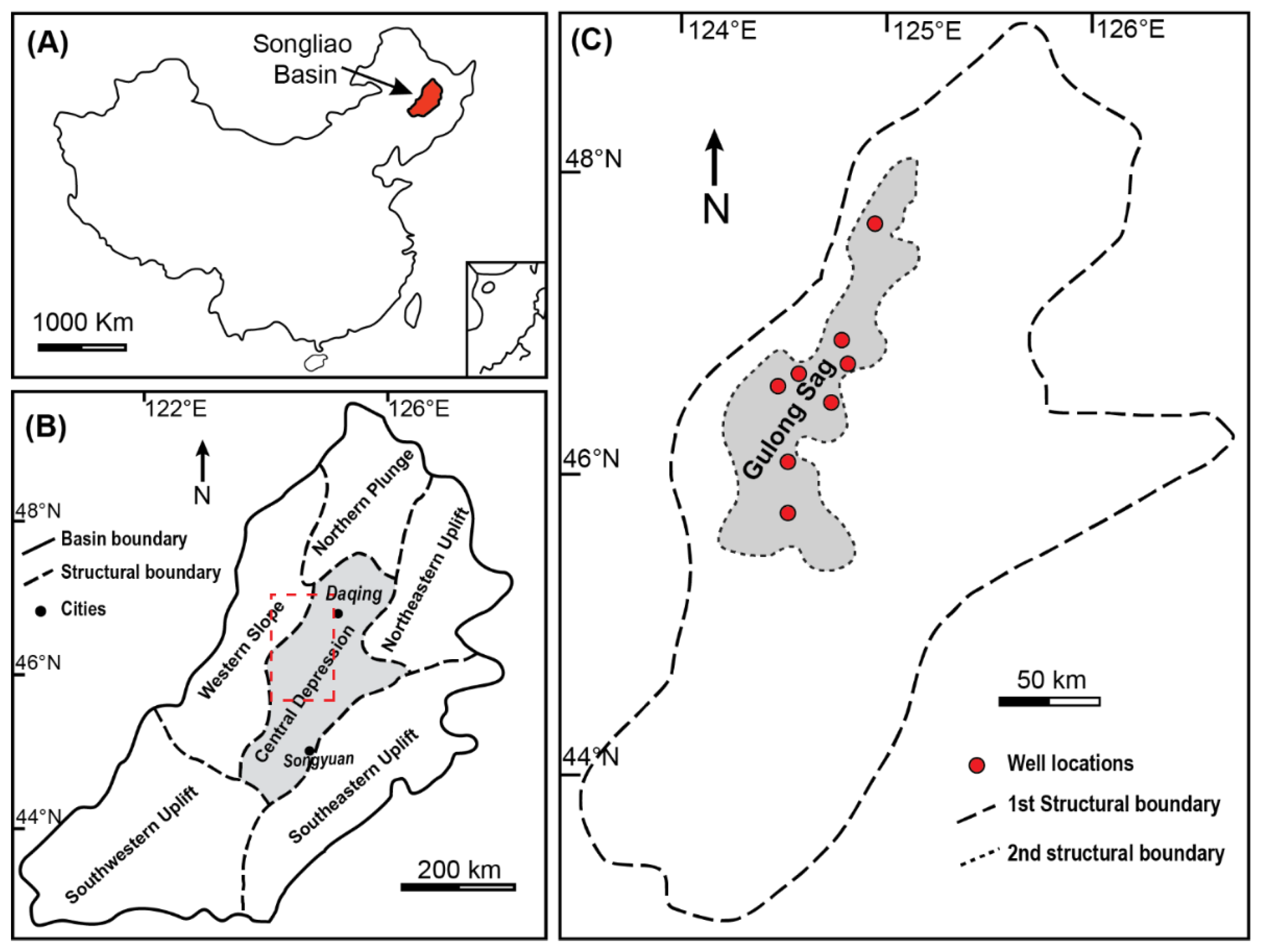
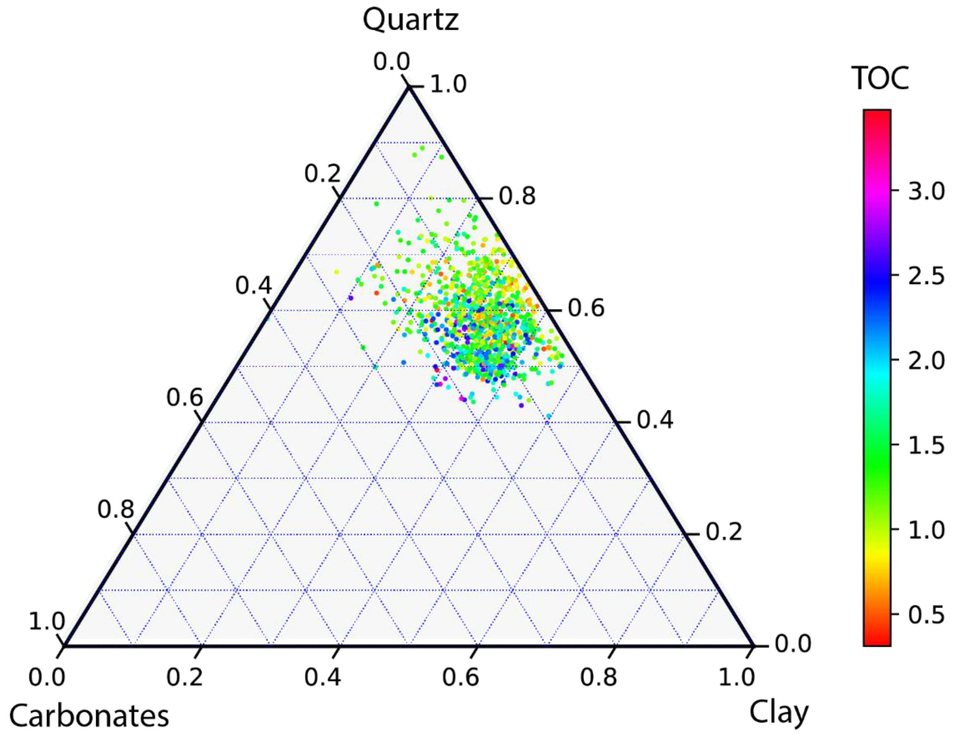
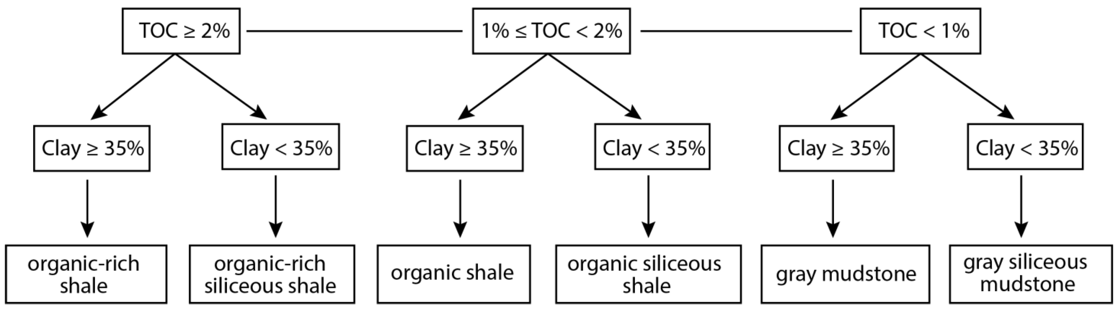
2. Geological Settings and Gulong Lithofacies

Songliao Basin, an intracratonic basin in north-eastern China, covers ~260,000 km², with a sizable sedimentary layer that is up to 6000 m thick and has been deposited since the Cretaceous period [39,40,41]. Gulong Shale was named after its location, the Gulong depression in the central area of Songliao Basin, occupying an area of ~3700 km² (Figure 2). In this study, Gulong Shale refers to the fine-grained sedimentary rocks of the upper Cretaceous Qingshankou Formation.

The Qingshankou Formation was deposited during the post-thermal subsidence stage [41,42] and has been one of the most important shale oil sources in China [10]. Its stratigraphy is subdivided into three members (K₂qn₁–K₂qn₃) from bottom to top. Oil shale succession is mainly preserved in the K₂qn₁ and K₂qn₂ members [10,43]. The first member (K₂qn₁) is represented by semi-deep and deep lacustrine deposits of grey/black and dark grey shale. It was developed during maximum lake expansion, with a thickness of 60–120 m. The second member (K₂qn₂) developed semi-deep lacustrine facies dominated by black and grey shale interlayered with thin siltstone and limestone. This study investigates the lithofacies of members one and two (K₂qn₁ and K₂qn₂, respectively) of the Qingshankou Formation.

Gulong Shale lithofacies has been classified based on TOC and XRD data from core geochemical analysis [10,11,12,17]. The K₂qn₁ and K₂qn₂ members of the Qingshankou Formation have TOC values ranging from 0.5% to 5.5%, with a mean of 1.9% and a clay volume ranging from 10% to 55%, with an average of 40% [10,11]. Overall, the Gulong Shale is rich in felsic components (quartz and feldspar) and clay minerals and is poor in carbonates (calcite and dolomite) (Figure 3). In this study, we applied a quantitative classification scheme based on TOC from laboratory examination and clay volume from ECS log (Figure 4). TOC > 2% is the cutoff for organic-rich shale, 1% < TOC < 2% is the cutoff for organic shale, and TOC < 1% is the cutoff for gray mudstone. Then, we subdivided the lithofacies with a 35% threshold for clay volume. Six lithofacies are classified for Gulong shale.

Organic-rich shale (ORS): This contains the highest organic matter (TOC ≥ 2%) and clay contents (clay ≥ 35%) among the six lithofacies of Gulong shale. It takes up to 12% of the total lithofacies. The well log characteristics are represented by high resistivity and high GR values.

Organic-rich siliceous shale (ORSS): This has the highest organic matter (TOC ≥ 2%), with clay contents of less than 35%. It holds the lowest proportion (5%) of the total lithofacies. The log curves are generally shown to have high resistivity values and lower GR values than ORS ones do.

Organic shale (OS): This is medium-rich in organic matters (1% ≤ TOC < 2%), with high clay contents (clay ≥ 35%). It is the most abundant one (taking up to 32%) among total lithofacies. The well log features exhibit medium-high resistivity values and high GR values.

Organic siliceous shale (OSS): This is medium-rich in organic matters (1% ≤ TOC < 2%), with clay contents of less than 35%. It is the second most abundant lithofacies, accounting for 29% of the total lithofacies. The log features are characterized by medium-high resistivity values and a lower GR than that of OS.

Gray mudstone (GM): This is poor in organic matter (TOC < 1%), but rich in clay contents (clay ≥ 35%). It takes up to 9% of the total lithofacies. The well log characteristics are represented by low resistivity and high GR values.

Gray siliceous mudstone (GSM): This is poor in organic matter, (TOC < 1%) with clay contents of less than 35%, represented by lower resistivity and GR values than those of the other lithofacies on the log curves. It accounts for 13% of the total lithofacies.

Overall, ORSS lithofacies (TOC ≥ 2% and clay < 35%) are relatively rare in the datasets. In contrast, OS (1% ≤ TOC < 2% and clay ≥ 35%) and OSS (1% ≤ TOC < 2% and clay < 35%) are most abundant ones. Classified lithofacies were calibrated with core-based ground truth information.

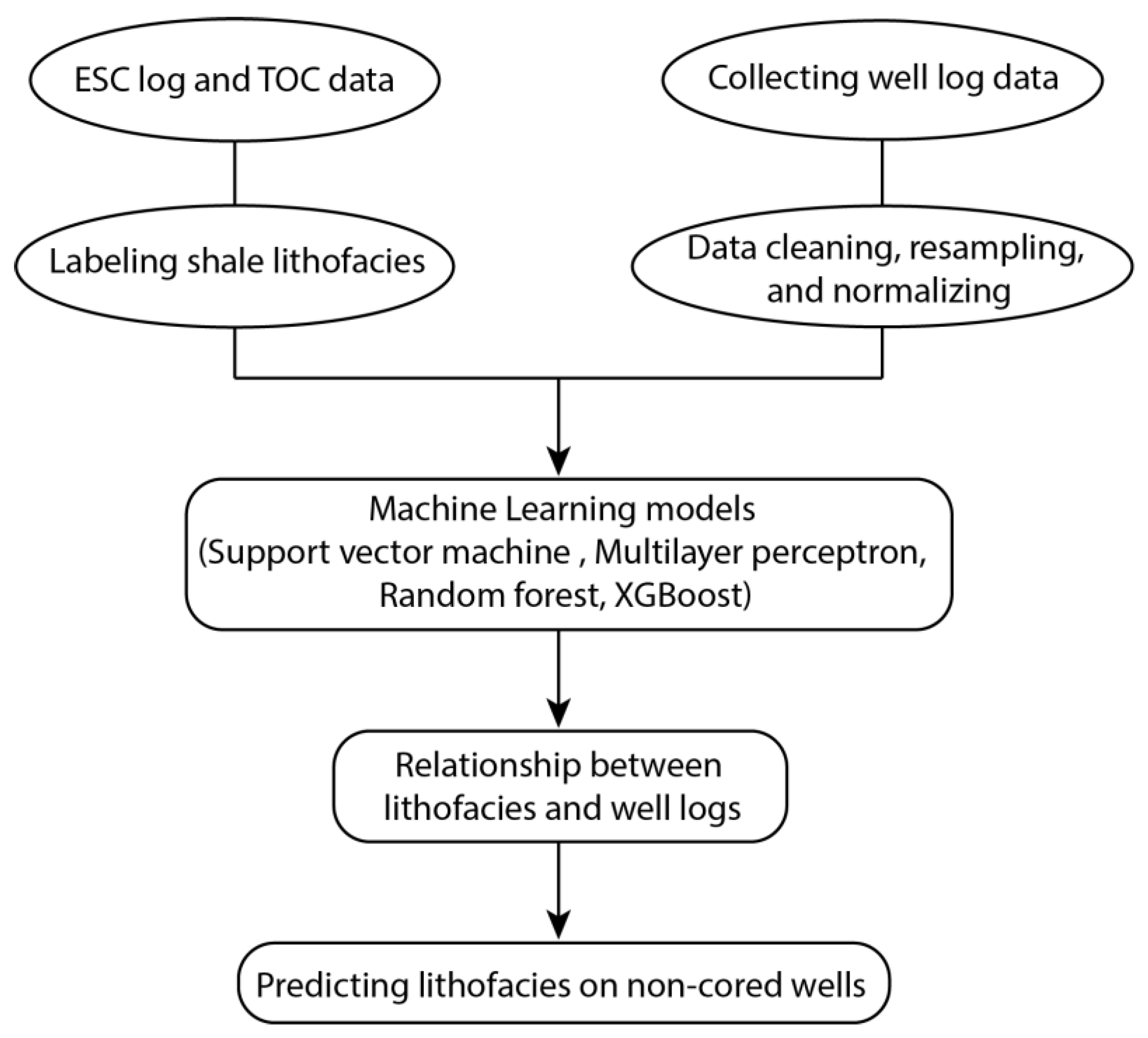
3. Materials and Methods

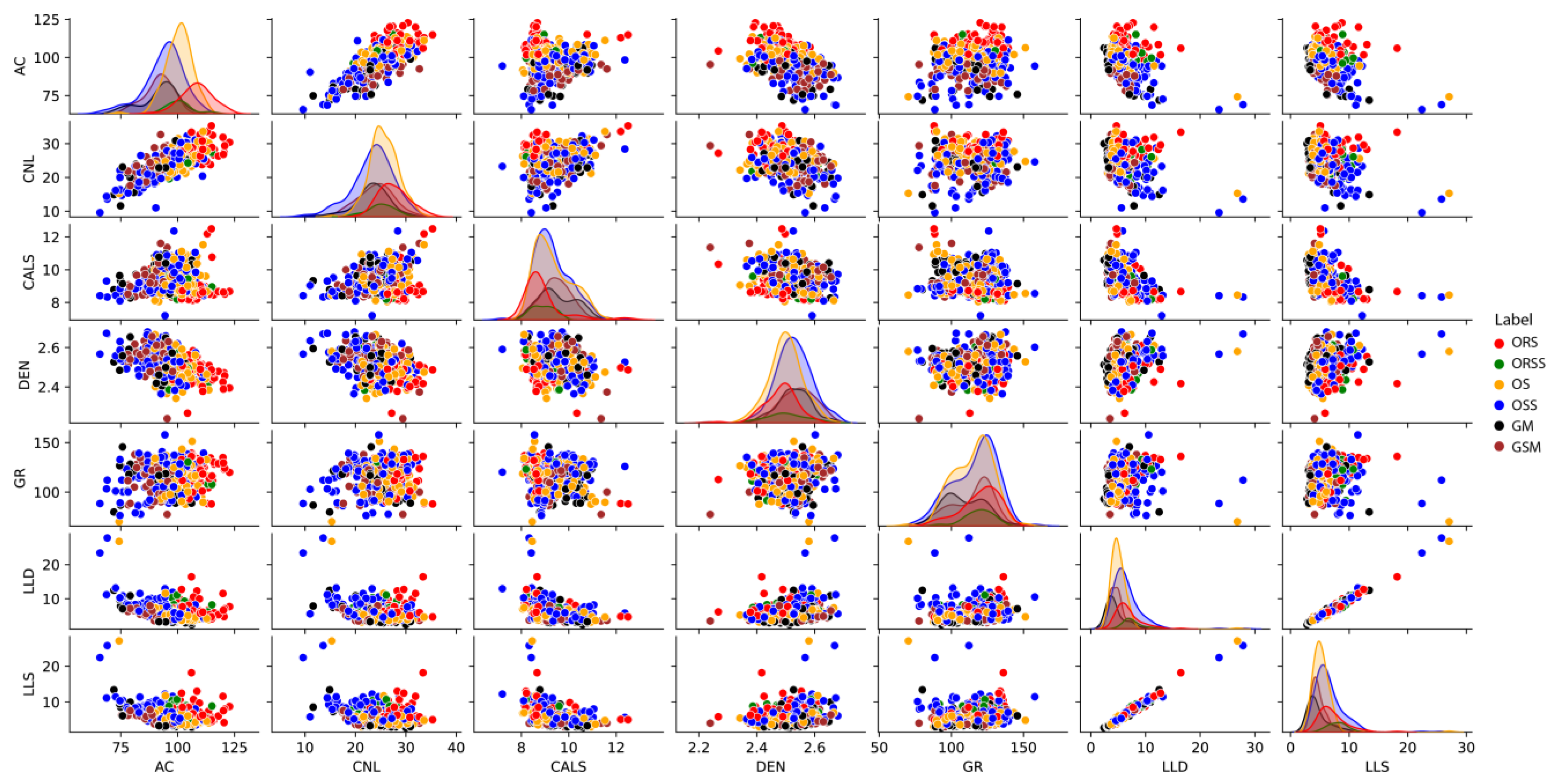
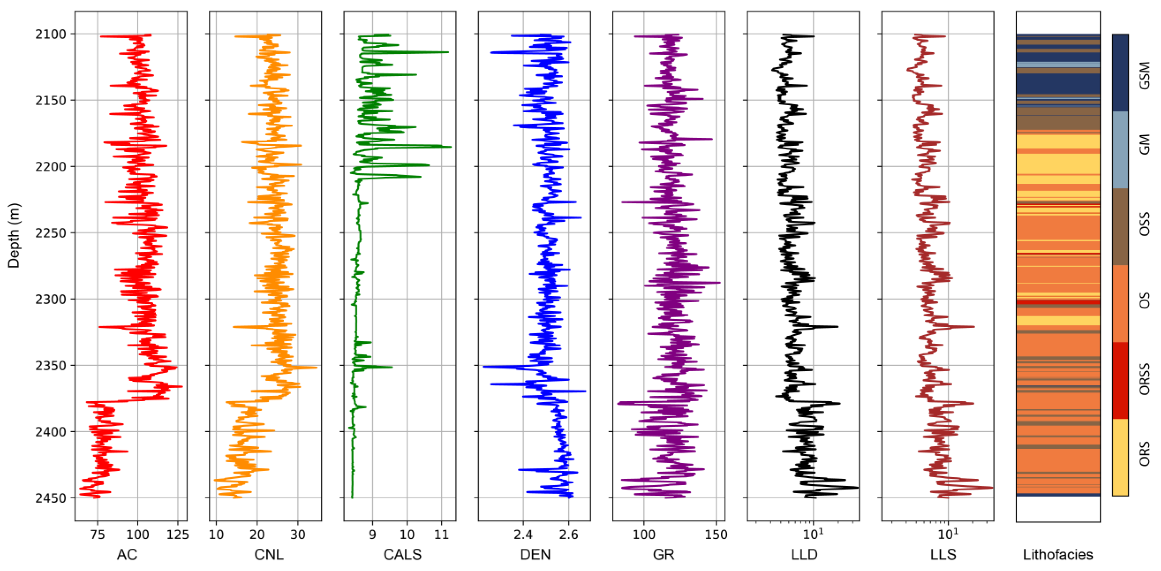
3.1. Selection of Well Logs

In this study, we chose seven conventional well logs (Figure 5 and Figure 6), including compensated neutron log (CNL), caliper log (CAL), density log (DEN), acoustic log (DT), gamma-ray log (GR), shallow laterolog resistivity log (LLS), and deep laterolog resistivity log (LLD), for lithofacies modeling. Well log data were collected from eight wells with a total thickness of 3426 m. The correlation between each two well logs was investigated by cross-plotting (Figure 5). The petrophysical properties of the well logs are as follows.

CNL log: This measures hydrogen concentration in a formation and operates by bombarding the formation with high-energy neutrons. Hydrogen may present as water or hydrocarbon in the pore spaces of reservoir rocks. As a result, the neutron energy loss can be associated with the porosity of a formation.

CAL log: this measures the size and shape of a borehole and can be an important indicator of shale swelling, washouts, and cave-ins in the boreholes.

DEN log: This compares the radiation sent from a Gamma source to those that are scattered back. It provides a formation’s bulk density consisting of rock density and fluid density contained in the pore spaces.

DT log: This measures the transit time of compressional sound waves to travel through the formation. It reflects lithological properties and is mainly used to calibrate seismic data and derive the density of a formation.

GR log: This measures the naturally occurring radiation of borehole rocks from potassium, thorium, and uranium isotopes. Clay has a high concentration of these isotopes, and thus can be distinguished by the Gamma log. The primary application of the Gamma log includes determining lithology, estimating shale content, and correlating the core with the logged depth.

Resistivity log: This measures the resistivities of subsurface formations, which depends on the resistivity of the formation water. It is a key parameter in determining the hydrocarbon saturation, water saturation, and porosity of a formation.

3.2. Well Log Data Processing

Data processing is requisite for training machine learning models. We selected oil-bearing layers of 8 wells to ensure all the data reflect the same geofluid conditions. Then, we cleaned the well log data by removing the invalid and missing values. Because different well logs have different magnitudes of values, all the data should be normalized to achieve similar magnitude and bias. The normalization scheme is as follows:

$$\mu =\frac{1}{n}{\displaystyle \sum }_{i=1}^n{x}_i$$

(1)

$$\sigma =\sqrt{\frac{1}{n-1}{\displaystyle \sum }_{i=1}^n{\left(x_i-\mu \right)}^2}$$

(2)

$$x_i^{\prime }=\frac{x_i-\mu }{\sigma }$$

(3)

where n is the number of samples; μ and σ are the mean and sample standard deviation of the samples; $x_i^{\prime }$ is the normalized value of $x_i$. After normalization, all types of well log data have a mean value of 0 and a standard deviation of 1.

3.3. Machine Learning Models

Machine learning has gained popularity in the last two decades in academic and industrial communities thanks to the rapid development of computing capabilities, especially in the GPU [45,46]. It is widely used in natural language processing, computer vision, and prediction tasks. Lithofacies prediction, in this study, utilized supervised learning, which generates prediction models based on training applied to labeled data. Each data point consists of a mapping between a feature vector and its labels, in other words, the desired output. Supervised learning algorithms infer parameters of artificial functions from the training data so that the realization of the cost function is minimized. With the inferred parameters, a model can be constructed to predict the output of new samples.

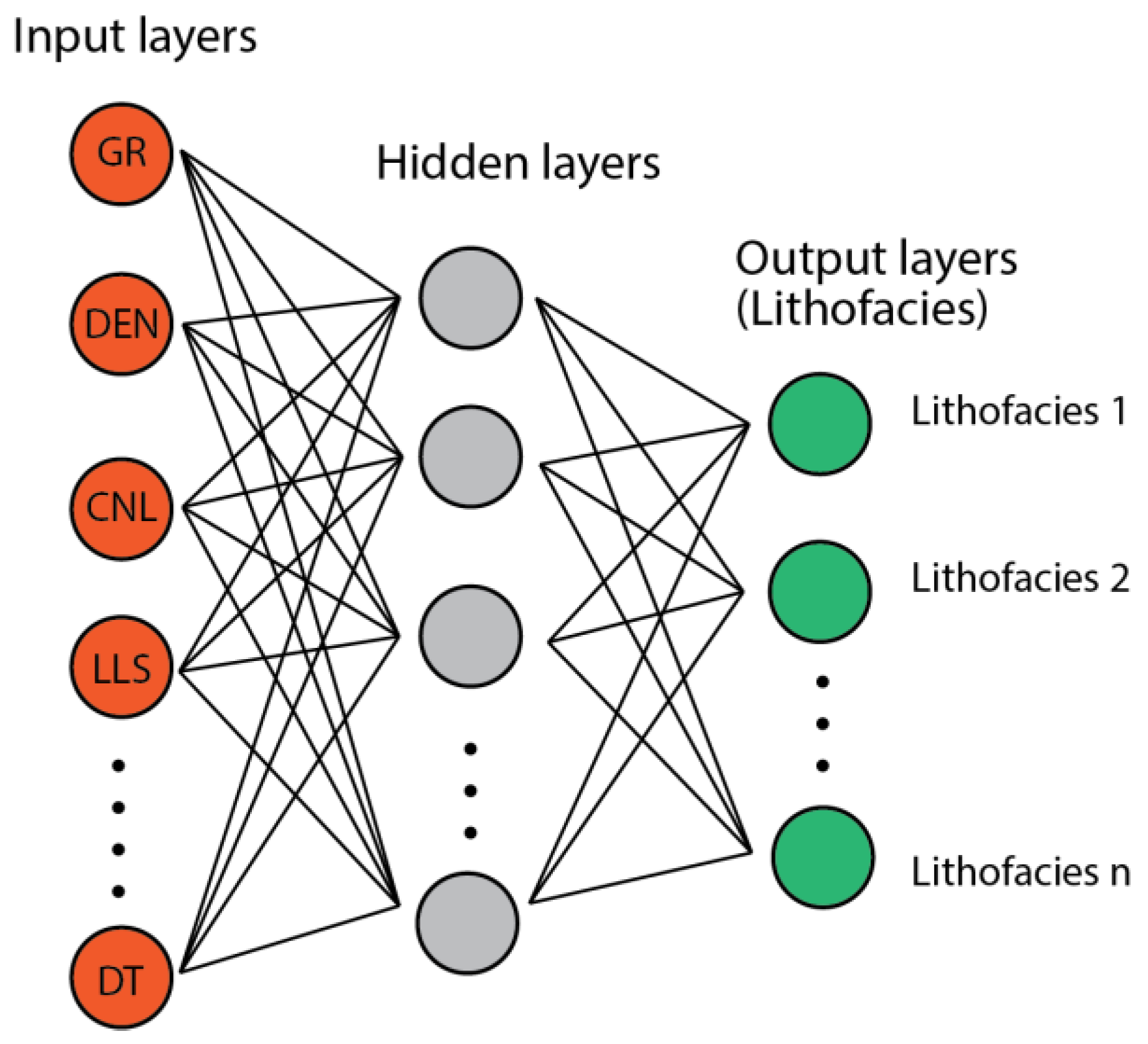
3.3.1. Multilayer Perceptron (MLP)

The MLP is a class of artificial neural networks with adjacent layers that are fully connected [47]. An MLP generally consists of three components: input layers, hidden layers, and output layers, where adjacent layers are connected by matrix multiplication (linear transformation) and nonlinear activation functions (Figure 7). The input layers retrieve the feature vectors from the dataset, and then send them to the hidden layers located between the input and output layers. In each hidden layer, the input data are applied with weights (affine transformation) and directed through a nonlinear transformation where the outputs are generated and sent to the next layers. The output size must be the same as the size of the next layer. The output layers are the last section of the feedforward process, where the prediction is obtained.

The value of the node is given by:

$$y=\sigma \left(w·x+b\right)$$

(4)

where σ represents the nonlinear activation function, $w$ represents the weight of the layer, $x$ represents the previous layer’s output, and $b$ represents the bias.

The backpropagation algorithm is the most widely used method to train an MLP model. The basic idea of backpropagation is to repeatedly adjust the weights of the layers to minimize a measure of the difference between the actual output vector and the desired output vector (cost functions). To determine the direction and magnitude of adjustments on weights, gradients of the cost function of parameters are computed with chain rules. Then, for each batch of data points in the training data sets, gradients are calculated and applied with the learning rate to the original weights, resulting in updated weights. By feeding the batches and executing the process iteratively, the cost function can be minimized such that the model will function well in the prediction task.

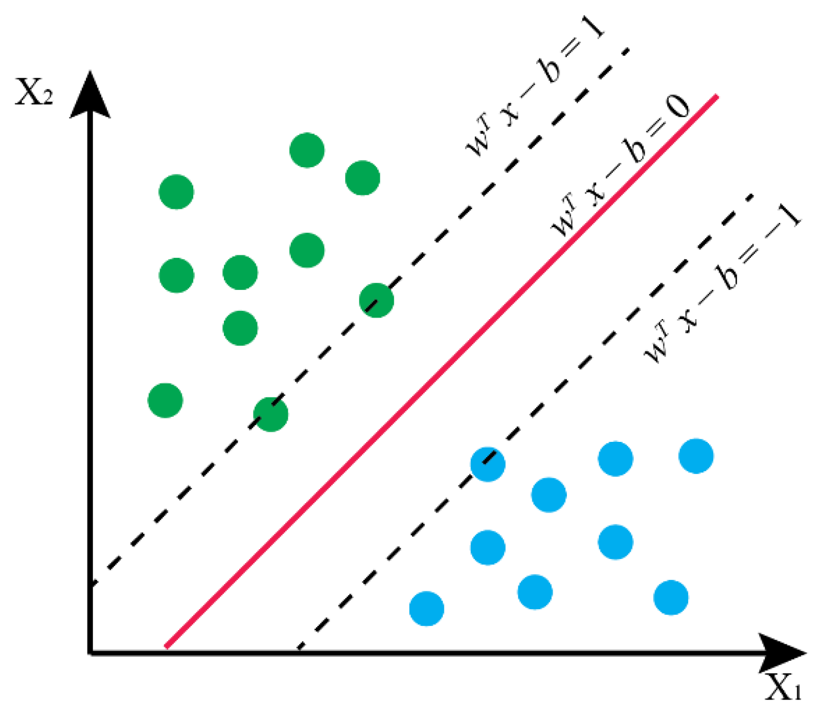
3.3.2. Support Vector Machine (SVM)

The SVM is a class of supervised learning algorithms that finds the optimal hyperplane or a set of hyperplanes that separate the data points in the high-dimensional feature space into different classes [48,49]. The best hyperplane is determined by the criteria that its distance from it to the nearest data point on each side is maximized (Figure 8).

Given n data points of {$\left(x_i,y_i\right)|i=1\dots n$}, where $x_i$ are the feature vectors and $y_i\in \left\{-1,1\right\}$ are the labels of the data points, a hyperplane can be written as $w^{T}x-b=0$, where $w$ is the normal vector to the hyperplane. Suppose the set of data points is linearly separable. In that case, two parallel hyperplanes can be selected such that data points with each class fall into different regions determined by the opposite sides of the two hyperplanes. Without the loss of generality, the two hyperplanes can be written as

$$w^{T}x-b=1$$

(5)

and

$$w^{T}x-b=-1$$

(6)

Their distance is $\frac{2}{\Vert w\Vert }$. The SVM aims to find the pair of parallel hyperplanes such that the distance between them is maximized.

The task of finding such hyperplanes can be formulated as a quadratic optimization problem:

• Minimize $\Vert w{\Vert }_2^2$
• Subject to: $y_i\left(w^T{x}_i-b\right)\ge 1, \forall i\in \left\{1,\dots ,n\right\}$

where $\Vert w{\Vert }_2$ is the L2 norm of $w$.

The formulation above assumes that the data points are linearly separable. However, in many datasets, the data points are not linearly separable, but can be separated by a nonlinear bound. To use SVM on these datasets, one can transform the feature space with a nonlinear kernel function such that the linear classifier SVM can potentially be applied to the transformed data points. Common kernels include the polynomial function (poly), Gaussian radial basis function (RBF), and sigmoid function.

3.3.3. Random Forest

Random Forest is an ensemble learning algorithm that constructs several decision trees and outputs the class that owns the majority vote of the trees [50]. It is an extension of the bootstrap aggregation algorithm. Unfortunately, the simple decision tree algorithm often overfits when the tree has grown very deep and learns irregular patterns. To overcome this shortcoming, the Random Forest combines the predictions from the trained trees with various subsets of the data so that the trees cancel out the irregular patterns.

The Random Forest algorithm begins with random sampling with replacement from the dataset and randomly selecting a subset of features. The randomness of the samples lowers the correlation between the trees and decreases the variance of the model, which helps to mitigate the overfitting effect. For the details of training a decision tree, the reader can refer to [51]. For IEEE transactions on systems, man, and cybernetics, see [51]. Next, each sample is used to train an individual decision tree. After training, a prediction can be made by selecting the majority vote of the decision trees given the same input.

3.3.4. Extreme Gradient Boosting (XGBoost)

Extreme Gradient Boosting (XGBoost) implements a gradient-boosting algorithm belonging to the ensemble learning family [52]. This implementation improves the efficiency and scalability more compared to that of the original gradient boosting algorithm. A gradient boosting algorithm accumulates weak learners, where they are generated sequentially based on the previous one, and finally, produces a strong learner. The weak learner is generated based on the residual of the previous learner, which is the difference between the actual and predicted values. As the boosting process continues, it gradually adjusts the model to improve its performance. In the optimization process of XGBoost, the second-order Taylor expansion is used to speed the convergence in the gradient descent. XGBoost also introduces regularization terms and shrinkage to control overfitting.

The gradient boosting iteration used in the XGBoost algorithm can be briefly illustrated as follows:

$$F_m\left(X\right)=F_{m-1}\left(X\right)+{\alpha }_m{h}_m\left(X,r_{m-1}\right)$$

where $F_m$ is the prediction model at the $m$th stage and $r_{m-1}$ is the computed residual of at the previous stage. $h_m$ is a function that is trained to predict the residual $r_m$. ${\alpha }_m$ is the regularization parameter, which is computed by $\underset{\alpha }{\mathrm{argmin}}{{\displaystyle \sum }}_{i=1}^{m}L(Y_i, F_{i-1}\left(X_i\right)+\alpha h_i\left(x_i,r_{i-1}\right)$, where $L\left(Y, F\left(X\right)\right)$ is a differentiable convex loss function for the residuals. In each iteration, a new tree that predicts the residuals of the prior trees is added to the model to make an updated prediction, and the loss functions for residuals are optimized with the gradient descent method. With the iterations continuing, the residuals can be compensated by the new tree iteratively.

3.3.5. Data Resampling, Tuning Processes, and Prediction Evaluation

In many circumstances, the training or test data sets are imbalanced, where the numbers of data points in each class are highly discrepant. The training process of the machine learning algorithms may suffer from an imbalance such that the decision function favors the classes with a great number of samples. To mitigate this issue, data resampling algorithms are developed and applied to data sets to reduce the impact caused by the imbalance. One widely used technique called oversampling is used to create synthetic data points for the classes with smaller sample sizes so that the numbers of samples in each class are balanced. There are two major algorithms for oversampling, Synthetic Minority Oversampling Technique (SMOTE) [53] and Adaptive Synthetic (ADASYN) [54]. Both algorithms were applied to the datasets before the training process. The performance of the two oversampling methods is reported later and compared with the result of the untreated data set.

In each machine learning model, several parameters define the architecture of models and the behavior of algorithms, which influences performance and efficiency. These parameters are called hyperparameters. Finding optimal values of the hyperparameters is the key to creating a useful model, where the optimal values may differ in different problems. Hyperparameter tuning is an exploration process that systematically searches the parameter space for a good setting. A naïve, but widely used, approach is the grid search, where the Cartesian product of all the candidates is explored. We used this approach to determine the optimal hyperparameter settings. The determined optimal hyperparameters were used in machine learning models for predicting Gulong Shale lithofacies.

There are several performance metrics to evaluate the classification model. These metrics include accuracy, precision, recall, and F1 score, defined as the following equations.

$$Accuracy=\frac{TP+TN}{TP+TN+FP+FN}$$

(7)

$$Precision=\frac{TP}{TP+FP}$$

(8)

$$Recall=\frac{TP}{TP+FN}$$

(9)

$$F1=\frac{2TP}{2TP+FP+FN}$$

(10)

TP, TN, FP, and FN stand for true positive, true negative, false positive, and false negative, respectively. Accuracy is the proportion of true results among the total examined samples. Precision is the proportion of predicted positive that is truly positive. The recall is the proportion of the correctly classified samples in the designated class. The F1 score is the harmonic mean of precision and recall, which measures the comprehensive goodness of the two metrics. All four metrics range from 0 to 1.

3.4. Overfitting and Cross-Validation

Overfitting may occur in the training process of supervised learning and needs to be prevented. An overfitted model fits well against the training data, but poorly against unseen data. As a result, the model lacks generalization capability and may fail to make reliable predictions on future observations. Early stopping, pruning, regularization, ensembling, and data augmentation are common approaches to prevent overfitting. In this study, we added regularization terms to the cost functions of SVM, Random Forest, and XGBoost algorithms and applied a 0.2 dropout rate to MLP to reduce the influence of overfitting.

K-fold cross-validation is widely used to detect overfitting. The dataset is shuffled and split evenly into k subsets called folds. The training process consists of a series of iterations. In each iteration, one fold is selected as the validation set, and the model is trained with the remaining k − 1 folds as the training set. The model is then evaluated and scored on the selected validation. The iterations repeat until all k folds have been selected as the validation set. The scores of all the iterations are averaged to illustrate the performance of the model. In our study, we used 5-fold cross-validation to obtain the assessment of the prediction models. In each iteration, precision, recall, and F1 score are calculated. They were averaged after all the iterations had been completed.

4. Results

All four machine learning algorithms were trained and tested using eight well logs. The hyperparameters were fine-tuned for each machine learning algorithm.

Table 1. Tuning parameters, candidates, and optimal values of each machine learning models.

Algorithms	Parameters	Candidates	Optimal Value
MLP	Number of hidden layers	1, 2	2
	Number of neurons in a hidden layer	10, 20, 50, 100	100
SVM	Kernel	Polynomial, Sigmoid, RBF	RBF
	Regularization	0.1, 1, 10	10
	Gamma	0.0001, 0.001, 0.1	0.1
XGBoost	Learning rate	0.01, 0.02, 0.05, 0.1	0.1
	Maximum child weight	1, 3, 5, 7	1
	Maximum tree depth	7, 9, 12, 15	15
Random Forest	Minimum samples split	2, 4, 7, 10	2
	Minimum samples leaf	1, 2, 5, 10, 20	1
	Maximum tree depth	5, 10, 15, 20	20

summarizes the tuning parameters, candidate values, and corresponding optimal values. All the trained models were evaluated on the test dataset for performance evaluation. The evaluation metrics include accuracy, precision, recall, and the F1 score. We tested SMOTE and ADASYN to select the better oversampling algorithm to be used for the data imbalance treatment. The comparison of performances of oversampling algorithms is shown in

Table 2. Comparison of the performances of oversampling algorithms.

Oversampling Algorithms	SVM	MLP	XGBoost	Random Forest
No sampling	0.708	0.810	0.845	0.875
SMOTE	0.723	0.809	0.868	0.884
ADASYN	0.693	0.794	0.853	0.870

.

4.1. Tuning Parameters

Table 1 summarizes the hyperparameters that were tuned, the candidate values, and the corresponding optimal values. The MLP performance depends on the number of hidden layers and neurons in hidden layers. Increasing the numbers of hidden layers and neurons improved the MLP performance. However, it takes more time and memory in the training process. The SVM algorithm achieves optimal performance using the RBF kernel function. Greater regularization and Gamma parameters also boosted the performance of SVM in our case. In the ensemble methods of XGBoost and Random Forest, deeper trees lead to better model performances with the cost of a longer training time and more memory utilization.

4.2. The Effect of Resampling on Imbalanced Datasets

The distribution of the Gulong Shale lithofacies is highly imbalanced (Figure 9). For example, the smallest class, ORSS, is about 5%, while the largest class, OS, takes up over 30%. To alleviate the prediction bias caused by imbalanced datasets, SMOTE and ADASYN oversampling methods were applied in the test run. As shown in Table 2, the ADASYN algorithm shows a slight improvement in the accuracy of the XGBoost model, but lower accuracies for SVM, MLP, and Random forest. The SMOTE algorithm shows slightly higher accuracy than the datasets without treatment do of up to 0.023. Since SMOTE was more effective in improving models’ performances, we used SMOTE for the data imbalance treatment before training.

4.3. Performances of Machine Learning Models

The performance matrix of SVM, MLP, XGBoost, and Random Forest is reported in

Table 3. Precision, recall and F1-scores for 5-fold-cross-validation over machine learning models.

	SVM			MLP			XGBoost			Random Forest
	Precision	Recall	F1-Score	Precision	Recall	F1-Score	Precision	Recall	F1-Score	Precision	Recall	F1-Score
ORS	0.808	0.777	0.792	0.871	0.857	0.864	0.923	0.925	0.924	0.932	0.920	0.926
ORSS	0.456	0.751	0.568	0.601	0.762	0.672	0.731	0.745	0.738	0.716	0.801	0.756
OS	0.793	0.750	0.771	0.850	0.819	0.835	0.904	0.887	0.895	0.917	0.909	0.913
OSS	0.746	0.663	0.702	0.798	0.778	0.788	0.858	0.847	0.853	0.894	0.861	0.877
GM	0.633	0.790	0.703	0.742	0.859	0.796	0.848	0.879	0.863	0.879	0.860	0.870
GSM	0.712	0.660	0.685	0.847	0.779	0.812	0.821	0.848	0.834	0.817	0.892	0.853
Average	0.691	0.732	0.704	0.785	0.809	0.794	0.847	0.855	0.851	0.859	0.874	0.866

. Overall, the two ensembled algorithms achieve significantly better results than SVM and MLP did. The Random Forest one shows superior performance among the four models, with an accuracy, precision, recall, and F1 scores on the test datasets of 0.884, 0.859, 0.874, and 0.866, respectively. Similar results are performed by XGBoost (0.868, 0.847, 0.855, and 0.851, respectively), which are better than those of the MLP model (0.809, 0.785, 0.809, and 0.794, respectively). The performance of SVM is poorer than those of the other three algorithms (0.723, 0.691, 0.732, and 0.704, respectively).

The confusion matrices of the four models are shown in Figure 10. ORS yields the highest precision among six lithofacies, with the best prediction of 0.932 performed by Random Forest. ORSS has the worst precisions, which are often mistakenly predicted as ORS, OS, or OSS ones. In the results of two ensembled models, the precisions of all the classes are above 0.8, except for ORSS.

5. Discussion

5.1. Comparison of the Performances of Machine Learning Models in Shale Lithofacies Prediction from Well Logs

The performances of ensemble methods (Random Forest and XGBoost) surpass those of MLP and SVM, with the highest accuracy of 0.884 predicted by Random Forest (Figure 10). SVM shows the lowest accuracy among the four models, with an accuracy of 0.723. For the Random Forest and XGBoost models, clay-rich lithofacies (ORS, OR, and GM) show a higher rate of accurate prediction than siliceous-rich lithofacies (ORSS, OSS, and GSM). This indicates that clay content is an important factor influencing the accuracy of lithofacies prediction from well logs. More than 80% of ORS can be predicted accurately in all four models, indicating that shale with high TOC and high clay contents has distinct features in the well log data, which makes it easier to be differentiated from other lithofacies. The lower rate of accurate prediction on ORSS may result from its feature that is not significant enough against ORS, OS, and OSS.

A test well is used to evaluate the generalization capability of the models. We used the random forest model, which has the best performance in our study, to predict the lithofacies along the depth of the test well. The comparison between the ground truth and predicted lithofacies is illustrated in Figure 11, and the performance matrix is reported in

Table 4. Precision, recall, and F1-score of Random forest model on a test well.

	Precision	Recall	F1-Score
ORS	0.847	0.835	0.841
ORSS	0.721	0.844	0.778
OS	0.836	0.835	0.835
OSS	0.917	0.89	0.903
GM	0.934	0.87	0.901
GSM	0.943	0.916	0.929
Average	0.866	0.865	0.865

. The accuracy of the random forest model on the test well is 0.867, indicating a great generalization performance. An interesting observation is that the prediction performance is significantly better on OSS, GM, and GSM.

In this study, the poorer performance of SVM than that of MLP is different from the observation of the Bakken and Marcellus Shale in the U.S., suggesting that the SVM algorithm outperforms ANN, SOM, and MRGC in lithofacies identification, with an accuracy of 0.825 [16]. This discrepancy is likely to be caused by the differences in shale mineralogy. Bakken and Marcellus Formations deposit marine, organic-rich (average TOC of 15%) shale [14,16,55]. The mineral composition is highly heterogenous, with average contents of quartz, clay, and carbonates of over 35%, 30%, and 25%, respectively. However, the Gulong Shale of the Qingshankou Formation is rich in quartz and clay (average of 60–75%) and poor in carbonate contents (average of 7%) [11,12]. The lithological composition of Gulong Shale is more homogenous than those of Bakken and Marcellus Shale. Hence, the variety of mineral compositions may affect the classifiers’ performance. A thorough analysis of the shale mineralogy would benefit the selection of classifiers for automated lithofacies prediction.

5.2. Prediction of Sweet Spots Based on Lithofacies Analysis

This study shows that ensemble machine learning models (Random Forest and XGBoost) are effective in identifying shale lithofacies from well logs, which can benefit the sweet spot prediction of shale reservoirs. The sedimentological, geochemical, and CT scanning studies have investigated the oil-bearing properties and favorable lithofacies of the Gulong Shale [10,11,18]. Among the six lithofacies classified in this study, organic siliceous shale has higher hydrocarbon generation potential and well-developed pore space, with macro-pores taking up to 21–48% of it [10]. The organic-rich shale and organic shale contain a relatively high TOC, but the pores are small and mostly isolated due to their high clay content. On the other hand, gray mudstone and siliceous mudstone have well-developed pores, but their hydrocarbon generation potential is low. Thus, organic siliceous shale is favorable lithofacies for the Gulong Shale of the Qingshankou Formation. The prediction accuracy of organic siliceous shale is 0.884 by Random Forest models, indicating that the machine learning model is capable of providing fast and efficient identification to favorable shale lithofacies of non-cored stratigraphy succession, and thus, benefit sweet spot prediction.

5.3. Future Works of Machine Learning Models for Lithofacies Prediction

The ensemble machine learning models in this study show advantages in predicting lithofacies and sweet spots of unconventional reservoirs with a high accuracy and low economic cost. However, more works are necessary to improve the model architecture. In this study, ORSS is often identified as ORS and OS, indicating that the current features from well logs are not sufficient at differentiating ORSS from other lithofacies. More input features are required to improve the model’s performance. Further improvements can be made from two aspects: adding domain knowledge and employing advanced well log data. Each type of depositional system has its unique lithological and lithofacies patterns. For example, a channel deposit of a fluvial system is characterized by an upward fining trend in grain size; a mouth bar of a deltaic system shows an upward coarsening pattern in the lithological column. Machine learning studies of fluvial lithofacies prediction have shown that the model accuracy increases by considering the vertical combination patterns of the lithology [30,56]. Hence, if some features of stacking patterns of shale lithofacies are added to models, the accuracy can be further improved. In addition to incorporate domain knowledge in the model, advanced well logs can bring additional geological information to enhance the prediction result. In shale reservoirs, the pores are generally rare, and the pore sizes are small, making conventional well logs difficult to provide accurate porosity estimations. As a result, nuclear magnetic resonance (NMR) logging has been increasingly embraced for its advantages in directly measuring porosity. Porosity-related parameters such as laminations and fractures implied by NMR logs can provide additional features for training models and potentially improve the performance. Other advanced well logs, such as borehole image logs providing structural and fracture analyses, may yield extra knowledge for lithofacies identification.

6. Conclusions

In this study, we examined the effectiveness of machine learning models in predicting clay-rich shale lithofacies from conventional well logs. We collected well log and TOC data from the Gulong Shale of the Qingshankou Formation in the Songliao Basin, China. ECS logs and TOC data were used to classify the Gulong Shale lithofacies into six groups. Four machine learning models (MLP, SVM, Random Forest, and XGBoost) were trained to identify the shale lithofacies from conventional well logs. Our major findings are as follows:

• Ensemble models (Random Forest and XGBoost) yield a better performance than the other models do for shale lithofacies identification. Random Forest conducts the best prediction with an accuracy of 0.884, precision of 0.859, recall of 0.874, and F1 score of 0.866.
• The differences in the models’ performances in predicting Gulong Shale and Bakken and Marcellus Shale in the previous studies may be due to the different mineral compositions. Our findings show that ensemble methods (Random Forest and XGBoost algorithms) are more suitable for classifying homogenous, clay-rich lithofacies such as Gulong Shale than the other models are.
• The performance of machine learning models on lithofacies prediction of shale can be associated with mineral composition. Understanding the characteristics of shale mineralogy is critical for choosing the appropriate classifiers for automated lithofacies prediction.
• Machine learning models have a large potential for identifying shale lithofacies of non-cored stratigraphic succession and predicting sweet spots of unconventional reservoirs. Further improvements in model performances can be achieved by adding domain knowledge and employing advanced well log data.

References

1. Wu, M.; Zhuang, G.; Hou, M.; Liu, Z. Expanded lacustrine sedimentation in the Qaidam Basin on the northern Tibetan Plateau: Manifestation of climatic wetting during the Oligocene icehouse. Earth Planet. Sci. Lett. 2021, 565, 116935. [Google Scholar] [CrossRef]
2. Hou, M.; Zhuang, G.; Ji, J.; Xiang, S.; Kong, W.; Cui, X.; Wu, M.; Hren, M. Profiling interactions between the Westerlies and Asian summer monsoons since 45 ka: Insights from biomarker, isotope, and numerical modeling studies in the Qaidam Basin. GSA Bull. 2020, 133, 1531–1541. [Google Scholar] [CrossRef]
3. Hou, M.; Zhuang, G.; Wu, M. Isotopic fingerprints of mountain uplift and global cooling in paleoclimatic and paleoecological records from the northern Tibetan Plateau. Palaeogeogr. Palaeoclimatol. Palaeoecol. 2021, 578, 110578. [Google Scholar] [CrossRef]
4. Bhattacharya, S.; Carr, T.; Wang, G. Shale lithofacies classification and modeling: Case studies from the Bakken and Marcellus formations, North America. In Proceedings of the AAPG Annual Convention and Exhibition, Denver, CO, USA, 31 May–3 June 2015. [Google Scholar]
5. Zou, C.; Feng, Y.; Yang, Z.; Jiang, W.; Pan, S.; Zhang, T.; Wang, X.; Zhu, J.; Li, J. What are the Lacustrine Fine-Grained Gravity Flow Sedimentation Process and the Genetic Mechanism of Sweet Sections for Shale Oil? J. Earth Sci. 2022, 33, 1321–1323. [Google Scholar] [CrossRef]
6. Hou, M.; Zhuang, G.; Ellwood, B.B.; Liu, X.-l.; Wu, M. Enhanced precipitation in the Gulf of Mexico during the Eocene–Oligocene transition driven by interhemispherical temperature asymmetry. GSA Bull. 2022, 134, 2335–2344. [Google Scholar] [CrossRef]
7. Slatt, R.M. Important geological properties of unconventional resource shales. Cent. Eur. J. Geosci. 2011, 3, 435–448. [Google Scholar] [CrossRef] [Green Version]
8. Law, B.E.; Curtis, J. Introduction to unconventional petroleum systems. AAPG Bull. 2002, 86, 1851–1852. [Google Scholar]
9. Zhan, C.; Sankaran, S.; LeMoine, V.; Graybill, J.; Mey, D.-O.S. Application of machine learning for production forecasting for unconventional resources. In Proceedings of the Unconventional Resources Technology Conference, Denver, CO, USA, 22–24 July 2019. [Google Scholar]
10. Liu, B.; Shi, J.; Fu, X.; Lyu, Y.; Sun, X.; Gong, L.; Bai, Y. Petrological characteristics and shale oil enrichment of lacustrine fine-grained sedimentary system: A case study of organic-rich shale in first member of Cretaceous Qingshankou Formation in Gulong Sag, Songliao Basin, NE China. Pet. Explor. Dev. 2018, 45, 884–894. [Google Scholar] [CrossRef]
11. Wang, L.; Zeng, W.; Xia, X.; Zhou, H.; Bi, H.; Shang, F.; Zhou, X. Study on lithofacies types and sedimentary environment of black shale of Qingshankou Formation in Qijia-Gulong Depression, Songliao Basin. Nat. Gas Geosci. 2019, 30, 1125–1133. [Google Scholar]
12. Jin, C.; Dong, W.; Bai, Y.; Lv, J.; Fu, X.; Li, J.; Ma, s. Lithofacies characteristics and genesis analysis of Gulong shale in Songliao Basin. Pet. Geol. Oilfield Dev. Daqing 2020, 39, 35–44. [Google Scholar]
13. He, W.; Meng, Q.; Zhang, J. Controlling factors and their classification-evaluation of Gulong shale oil enrichment in Songliao Basin. Pet. Geol. Oilfield Dev. Daqing 2021, 40, 1–12. [Google Scholar]
14. Wang, G.; Carr, T.R. Marcellus Shale Lithofacies Prediction by Multiclass Neural Network Classification in the Appalachian Basin. Math. Geosci. 2012, 44, 975–1004. [Google Scholar] [CrossRef]
15. Wang, G.; Carr, T.R. Organic-rich Marcellus Shale lithofacies modeling and distribution pattern analysis in the Appalachian Basin. AAPG Bull. 2013, 97, 2173–2205. [Google Scholar] [CrossRef] [Green Version]
16. Bhattacharya, S.; Carr, T.R.; Pal, M. Comparison of supervised and unsupervised approaches for mudstone lithofacies classification: Case studies from the Bakken and Mahantango-Marcellus Shale, USA. J. Nat. Gas Sci. Eng. 2016, 33, 1119–1133. [Google Scholar] [CrossRef] [Green Version]
17. Gao, B.; He, W.; Feng, Z.; Shao, H.; Zhang, A.; Pan, H.; Chen, G. Lithology, physical property, oil-bearing property and their controlling factors of Gulong shale in Songliao Basin. Pet. Geol. Oilfield Dev. Daqing 2022, 41, 68–79. [Google Scholar]
18. Cui, B.; Chen, C.; Lin, X.; Zhao, Y.; Cheng, X.; Zhang, Y.; Lu, G. Characteristics and distribution of sweet spots in Gulong shale oil reserviors of Songliao Basin. Pet. Geol. Oilfield Dev. Daqing 2020, 39, 45–55. [Google Scholar]
19. Busch, J.; Fortney, W.; Berry, L. Determination of lithology from well logs by statistical analysis. SPE Form. Eval. 1987, 2, 412–418. [Google Scholar] [CrossRef]
20. Ellis, D.V.; Singer, J.M. Well Logging for Earth Scientists; Springer: Berlin/Heidelberg, Germany, 2007; Volume 692. [Google Scholar]
21. Asquith, G.B.; Krygowski, D.; Gibson, C.R. Basic Well Log Analysis; American Association of Petroleum Geologists: Tulsa, OK, USA, 2004; Volume 16. [Google Scholar]
22. Song, S.; Mukerji, T.; Hou, J.; Zhang, D.; Lyu, X. GANSim-3D for Conditional Geomodeling: Theory and Field Application. Water Resour. Res. 2022, 58, e2021WR031865. [Google Scholar] [CrossRef]
23. Song, S.; Mukerji, T.; Hou, J. GANSim: Conditional facies simulation using an improved progressive growing of generative adversarial networks (GANs). Math. Geosci. 2021, 53, 1413–1444. [Google Scholar] [CrossRef]
24. Ashraf, U.; Zhang, H.; Anees, A.; Mangi, H.N.; Ali, M.; Zhang, X.; Imraz, M.; Abbasi, S.S.; Abbas, A.; Ullah, Z. A core logging, machine learning and geostatistical modeling interactive approach for subsurface imaging of lenticular geobodies in a clastic depositional system, SE Pakistan. Nat. Resour. Res. 2021, 30, 2807–2830. [Google Scholar] [CrossRef]
25. Ali, M.; Jiang, R.; Ma, H.; Pan, H.; Abbas, K.; Ashraf, U.; Ullah, J. Machine learning-A novel approach of well logs similarity based on synchronization measures to predict shear sonic logs. J. Pet. Sci. Eng. 2021, 203, 108602. [Google Scholar] [CrossRef]
26. Raeesi, M.; Moradzadeh, A.; Doulati Ardejani, F.; Rahimi, M. Classification and identification of hydrocarbon reservoir lithofacies and their heterogeneity using seismic attributes, logs data and artificial neural networks. J. Pet. Sci. Eng. 2012, 82–83, 151–165. [Google Scholar] [CrossRef]
27. Rogers, S.J.; Fang, J.; Karr, C.; Stanley, D. Determination of lithology from well logs using a neural network. AAPG Bull. 1992, 76, 731–739. [Google Scholar]
28. Al-Mudhafar, W.J. Integrating well log interpretations for lithofacies classification and permeability modeling through advanced machine learning algorithms. J. Pet. Explor. Prod. Technol. 2017, 7, 1023–1033. [Google Scholar] [CrossRef] [Green Version]
29. Zheng, D.; Hou, M.; Chen, A.; Zhong, H.; Qi, Z.; Ren, Q.; You, J.; Wang, H.; Ma, C. Application of machine learning in the identification of fluvial-lacustrine lithofacies from well logs: A case study from Sichuan Basin, China. J. Pet. Sci. Eng. 2022, 215, 110610. [Google Scholar] [CrossRef]
30. Ren, X.; Hou, J.; Song, S.; Liu, Y.; Chen, D.; Wang, X.; Dou, L. Lithology identification using well logs: A method by integrating artificial neural networks and sedimentary patterns. J. Pet. Sci. Eng. 2019, 182, 106336. [Google Scholar] [CrossRef]
31. Xie, Y.; Zhu, C.; Zhou, W.; Li, Z.; Liu, X.; Tu, M. Evaluation of machine learning methods for formation lithology identification: A comparison of tuning processes and model performances. J. Pet. Sci. Eng. 2018, 160, 182–193. [Google Scholar] [CrossRef]
32. Ippolito, M.; Ferguson, J.; Jenson, F. Improving facies prediction by combining supervised and unsupervised learning methods. J. Pet. Sci. Eng. 2021, 200, 108300. [Google Scholar] [CrossRef]
33. Ehsan, M.; Gu, H. An integrated approach for the identification of lithofacies and clay mineralogy through Neuro-Fuzzy, cross plot, and statistical analyses, from well log data. J. Earth Syst. Sci. 2020, 129, 1–13. [Google Scholar] [CrossRef]
34. Khalil Khan, H.; Ehsan, M.; Ali, A.; Amer, M.A.; Aziz, H.; Khan, A.; Bashir, Y.; Abu-Alam, T.; Abioui, M. Source rock geochemical assessment and estimation of TOC using well logs and geochemical data of Talhar Shale, Southern Indus Basin, Pakistan. Front. Earth Sci. 2022, 1593, 969936. [Google Scholar] [CrossRef]
35. Merembayev, T.; Kurmangaliyev, D.; Bekbauov, B.; Amanbek, Y. A Comparison of Machine Learning Algorithms in Predicting Lithofacies: Case Studies from Norway and Kazakhstan. Energies 2021, 14, 1896. [Google Scholar] [CrossRef]
36. Manzoor, U.; Ehsan, M.; Radwan, A.E.; Hussain, M.; Iftikhar, M.K.; Arshad, F. Seismic driven reservoir classification using advanced machine learning algorithms: A case study from the lower Ranikot/Khadro sandstone gas reservoir, Kirthar fold belt, lower Indus Basin, Pakistan. Geoenergy Sci. Eng. 2023, 222, 211451. [Google Scholar] [CrossRef]
37. Safaei-Farouji, M.; Thanh, H.V.; Dashtgoli, D.S.; Yasin, Q.; Radwan, A.E.; Ashraf, U.; Lee, K.-K. Application of robust intelligent schemes for accurate modelling interfacial tension of CO2 brine systems: Implications for structural CO2 trapping. Fuel 2022, 319, 123821. [Google Scholar] [CrossRef]
38. Tewari, S.; Dwivedi, U.D. Ensemble-based big data analytics of lithofacies for automatic development of petroleum reservoirs. Comput. Ind. Eng. 2019, 128, 937–947. [Google Scholar] [CrossRef]
39. Wang, P.-J.; Mattern, F.; Didenko, N.A.; Zhu, D.-F.; Singer, B.; Sun, X.-M. Tectonics and cycle system of the Cretaceous Songliao Basin: An inverted active continental margin basin. Earth Sci. Rev. 2016, 159, 82–102. [Google Scholar] [CrossRef] [Green Version]
40. Gao, R.; Zhang, Y.; Cui, T. Cretaceous Petroleum Bearing Strata in the Songliao Basin; Petroleum Industry Press: Beijing, China, 1994. [Google Scholar]
41. Wu, H.; Zhang, S.; Jiang, G.; Huang, Q. The floating astronomical time scale for the terrestrial Late Cretaceous Qingshankou Formation from the Songliao Basin of Northeast China and its stratigraphic and paleoclimate implications. Earth Planet. Sci. Lett. 2009, 278, 308–323. [Google Scholar] [CrossRef]
42. Xu, J.; Liu, Z.; Bechtel, A.; Meng, Q.; Sun, P.; Jia, J.; Cheng, L.; Song, Y. Basin evolution and oil shale deposition during Upper Cretaceous in the Songliao Basin (NE China): Implications from sequence stratigraphy and geochemistry. Int. J. Coal Geol. 2015, 149, 9–23. [Google Scholar] [CrossRef]
43. Wang, Y.; Liang, J.; Zhang, J. Resource potential and exploration direction of Gulong shale oil in Songliao Basin. Pet. Geol. Oilfield Dev. Daqing 2020, 39, 20–34. [Google Scholar]
44. Liu, B.; Wang, H.; Fu, X.; Bai, Y.; Bai, L.; Jia, M.; He, B. Lithofacies and depositional setting of a highly prospective lacustrine shale oil succession from the Upper Cretaceous Qingshankou Formation in the Gulong sag, northern Songliao Basin, northeast China. AAPG Bull. 2019, 103, 405–432. [Google Scholar] [CrossRef] [Green Version]
45. Mahesh, B. Machine learning algorithms-a review. Int. J. Sci. Res. 2020, 9, 381–386. [Google Scholar]
46. Jordan, M.I.; Mitchell, T.M. Machine learning: Trends, perspectives, and prospects. Science 2015, 349, 255–260. [Google Scholar] [CrossRef]
47. Bishop, C.M. Neural Networks for Pattern Recognition; Oxford University Press: Oxford, UK, 1995. [Google Scholar]
48. Hearst, M.A.; Dumais, S.T.; Osuna, E.; Platt, J.; Scholkopf, B. Support vector machines. IEEE Intell. Syst. Appl. 1998, 13, 18–28. [Google Scholar] [CrossRef] [Green Version]
49. Vapnik, V. The Nature of Statistical Learning Theory; Springer Science & Business Media: Berlin/Heidelberg, Germany, 1999. [Google Scholar]
50. Ho, T.K. Random decision forests. In Proceedings of the 3rd International Conference on Document Analysis and Recognition, Montreal, QC, Canada, 14–16 August 1995. [Google Scholar]
51. Safavian, S.R.; Landgrebe, D. A survey of decision tree classifier methodology. IEEE Trans. Syst. Man Cybern. 1991, 21, 660–674. [Google Scholar] [CrossRef] [Green Version]
52. Chen, T.; Guestrin, C. Xgboost: A scalable tree boosting system. In Proceedings of the 22nd ACM SIGKDD International Conference on Knowledge Discovery and Data Mining, San Francisco, CA, USA, 13–17 August 2016. [Google Scholar]
53. Chawla, N.V.; Bowyer, K.W.; Hall, L.O.; Kegelmeyer, W.P. SMOTE: Synthetic minority over-sampling technique. J. Artif. Intell. Res. 2002, 16, 321–357. [Google Scholar] [CrossRef]
54. He, H.; Bai, Y.; Garcia, E.A.; Li, S. ADASYN: Adaptive synthetic sampling approach for imbalanced learning. In Proceedings of the 2008 IEEE International Joint Conference on Neural Networks (IEEE World Congress on Computational Intelligence), Hong Kong, China, 1–8 June 2008. [Google Scholar]
55. Hackley, P.C.; Cardott, B.J. Application of organic petrography in North American shale petroleum systems: A review. Int. J. Coal Geol. 2016, 163, 8–51. [Google Scholar] [CrossRef] [Green Version]
56. Song, S.; Hou, J.; Dou, L.; Song, Z.; Sun, S. Geologist-level wireline log shape identification with recurrent neural networks. Comput. Geosci. 2020, 134, 104313. [Google Scholar] [CrossRef]
Figure 1. The flowchart illustrates the workflow of this study. Refer to the text for abbreviations of well logs and models.
Energies 16 02581 g001
Figure 2. Geological Maps showing the study area (modified from Liu et al. 2019 [44]). (A) Location of Songliao Basin. (B) Tectonic divisions of the Songliao Basin Central depression, with a shaded area representing the central depression. The red square denotes the study area in Figure 2C. (C) The 1st-order structural boundary outlines the central depression, and the 2nd-order structural boundary constraints Gulong Sag (shaded area); studied wells are shown in red circles.
Energies 16 02581 g002
Figure 3. A ternary plot showing percentages of three major components (i.e., quartz, carbonates, and clay) of Gulong shale from the Qingshankou Formation. Data are adapted from [10,11,12].
Energies 16 02581 g003
Figure 4. Tree diagram showing the criteria for classifying Gulong Shale lithofacies.
Energies 16 02581 g004
Figure 5. Cross plots of seven well logs, with six lithofacies represented by different colors. Six lithofacies are identified in the Gulong Shale, including organic-rich shale (ORS), organic-rich siliceous shale (ORSS), organic shale (OS), organic siliceous shale (OSS), gray mudstone (GM), and gray siliceous mudstone (GSM). Refer to the text for abbreviations of well logs.
Energies 16 02581 g005
Figure 6. Integrated well logs and lithofacies model of the Qingshankou Formation in one of the training wells. Shale lithofacies were classified using elemental capture spectroscopy logs (ECS) and measured TOC data. See the text for abbreviations of lithofacies and well logs.
Energies 16 02581 g006
Figure 7. A Multilayer Perceptron (MLP) schematic diagram where inputs stand for well logs and outputs represent different lithofacies.
Energies 16 02581 g007
Figure 8. A schematic diagram showing a hyperplane (redline) that separates data points (green and blue dots) from two classes with maximum margin.
Energies 16 02581 g008
Figure 9. Distributions of the Gulong lithofacies in the datasets. Refer to text for abbreviations of lithofacies.
Energies 16 02581 g009
Figure 10. Confusion matrix of lithofacies prediction on test datasets by MLP (a), SVM (b), Random Forest (c), and XGBoost models (d). Refer to text for abbreviations of lithofacies.
Energies 16 02581 g010
Figure 11. Lithofacies prediction by Random Forest model on a test well in the study area. Refer to the text for abbreviations of lithofacies and well logs.
Energies 16 02581 g011