A Position-Insensitive Nonlinear Inductive Power Transfer System Employing Saturable Inductor

Abstract

Most of the practical inductive power transfer (IPT) systems are the ones with variable coupling coefficients and loads. The output voltage, current and power are affected by the variation in coupling coefficient and load. In this paper, a novel approach based on a nonlinear resonator is proposed to obtain stable output voltage, which is independent of coupling coefficient and load variation. First, the theory and properties of nonlinear resonators are analyzed by Duffing equation. Then, a nonlinear IPT system with a magnetic saturation inductor is proposed, and the saturable inductor modeling and its effect on system performance are further studied. Finally, the experimental prototype is built to validate the effectiveness of the nonlinear IPT system. The experimental results show that when the coupling coefficient varies from 0.32 to 0.24 and the load resistance varies from $80\mathrm{\Omega }$ to $120\mathrm{\Omega }$, the system works in a nonlinear state, the output voltage ripple is 1.77%, and the overall efficiency of the system is not less than 82.60%. The experimental results are basically consistent with the theoretical analysis. The novel design approach improves the output voltage stability with respect to position misalignment and load variation, and the bandwidth of the system is also enhanced.

1. Introduction

Inductive power transfer (IPT) is a burgeoning technology that can wirelessly transfer electrical energy over a certain distance, which has some remarkable properties in terms of safety, flexibility and reliability [1]. The application purpose of the IPT system is to make the power supply more flexible and convenient. If the position-insensitive performance of the system is insufficient, it is difficult to satisfy the requirements of practical applications, such as electric vehicles, consumer electronics and medical electronics. Therefore, improving the anti-misalignment ability of the IPT system has become a research hotspot [2,3].

As shown in Figure 1, the IPT system consists of a power supply, power conversion module, compensation network, magnetic coupling mechanism and load. The anti-misalignment strategies are mainly classified into three categories: magnetic coupling coils design and optimization, control strategy and compensation topology. The transmitting and receiving coils are key components of the IPT system; many types of magnetic coupling coils have been proposed, such as double D quadrature (DDQ) coils [4], bipolar (BP) coils [5], tripolar (TP) coils [6], etc. In most of the magnetic couplers, the magnetic flux is guided and shielded using a high-conductivity ferrite core and an aluminum plate, respectively [7]. However, if only the magnetic coupling mechanism is designed and optimized, the loss and volume of the magnetic coupling mechanism will be increased, and the anti-misalignment ability of the system will be limited. The power conversion modules are connected from the power supply to load successively, and the power variation of each module directly affects the output of the IPT system. Therefore, the system output can be adjusted through control strategies, which can be classified into three main groups: primary-side control [8,9], secondary-side control [10,11] and dual-control [12,13]. The control strategy can accurately control the output of the system, but the complexity of the system increases, and the reliability decreases. The compensation topologies with anti-misalignment ability can be classified into three structures: higher-order topologies [14,15], hybrid topologies [16,17] and reconfigurable topologies [18,19]. However, the anti-misalignment ability of higher-order topologies is limited, the number of coils and compensating elements of the hybrid topology is increased, additional auxiliary circuits and control strategies are required for reconfigurable topologies.

A wireless power transfer (WPT) system with a nonlinear resonator (also known as the Duffing resonator) is proposed in Refs. [20,21,22]. The Duffing resonator is composed of a nonlinear capacitor and receiving coil inductance, which can improve the position-insensitive ability of the WPT system. A WPT system employing parity-time symmetric Duffing resonator is proposed in [23,24]. The nonlinear resonator consists of a nonlinear capacitor and negative resistor, which can improve the bandwidth and position-insensitive ability of the WPT system. The nonlinear resonators in the above schemes are composed of nonlinear capacitors and linear inductors, and the nonlinear capacitors are built by analog circuits [25]. It is difficult to realize in practical applications and is not suitable for low-frequency and high-power IPT systems.

The above nonlinear compensation topology solves the problem of output instability caused by coupling coefficient variation and frequency drift of the IPT system. However, there are still some other problems, such as the nonlinear component structure being complex, the system transfer power is not high and the need for additional sensors and controllers. Therefore, a novel nonlinear IPT system is designed by using a saturable inductor. The LCC topology is selected as the primary compensation to ensure that the transmitting coil current is independent of the receiver. The capacitors and saturable inductor are connected in parallel to form a compensation network of the secondary side to ensure that the IPT system can work in a nonlinear resonant state. As long as the proposed IPT system enters the nonlinear resonance state, the output voltage can remain essentially constant, even if the coupling coefficient or equivalent load varies within a certain range. In addition, the bandwidth of the IPT system is improved by introducing the saturable inductor.

The rest of this paper is organized as follows. The theory and properties of the nonlinear resonator are discussed in Section 2. The proposed topology and operation are analyzed in Section 3. Experimental validation and further discussion are presented in Section 4. The conclusions are outlined in Section 5.

2. Theory and Properties of Nonlinear Resonator

Duffing nonlinear, named after Georg Duffing, is one of the most widely studied nonlinear vibration phenomena in a number of fields, such as mathematics, physics and mechanical engineering. Many mathematical models of nonlinear vibration problems in engineering applications can be transformed into a Duffing equation, which is also very significant for the research of some problems in the field of electrical engineering [26,27]. Its standard form is:

$$\begin{array}{c}\hfill \ddot{x}+\beta \dot{x}+{\omega }_0^{2}x+\alpha x^3=Fcos\omega t.\end{array}$$

(1)

where x represents displacement, $\beta$ represents the damping coefficient, ${\omega }_0$ represents the natural resonant angular frequency, $\alpha$ represents the third-order nonlinear coefficient and $Fcos\left(\omega t\right)$ represents the excitation that has an excitation amplitude F and power angular frequency $\omega$. The approximate steady-state solution of Equation (1) can be described as

$$\begin{array}{c}\hfill a(\omega ,t)=A\left(\omega \right)cos(\omega t-\theta ).\end{array}$$

(2)

where A is the response amplitude and $\theta$ is the phase shift with respect to the power source. The response amplitude can be determined from

$$\begin{array}{c}\hfill A^2{[({\omega }_0^2-{\omega }^2)+0.75\alpha A^2]}^2+{\left(\beta A\omega \right)}^2=F^2.\end{array}$$

(3)

As shown in Figure 2a, the amplitude-frequency response curves of the linear resonator and Duffing resonator are depicted. It can be seen that the curve of the linear resonator is centered symmetrically, while the response curve of the nonlinear resonator is tilted to the right, which is called the hysteresis characteristic. Therefore, there are three different response values within a specific frequency range. Here, the middle points are unstable, and the upper and lower equilibrium points are stable. Assuming that the excitation amplitude remains unchanged, the response amplitude varies along points 1, 2, 3, 4, 5 when the frequency f increases slowly and jumps from point 3 to point 4. On the contrary, when f decreases slowly, the response amplitude changes along points 5, 4, 6, 7, 2, 1 and jumps from point 6 to point 7. Here, points 3 and 6 are called jumping points; the corresponding frequencies are boundary frequencies, this behavior is known as jumping characteristics [28].

As shown in Figure 2b, the amplitude-frequency response curves are dependent on third-order nonlinear coefficients $\alpha$. The curve is centered symmetrically when $\alpha =0$, which is called a linear system. The curve is tilted to the right side when $\alpha >0$, which is called a hardening system. The curve is tilted to the left side when $\alpha <0$, which is called a softening system [29]. The bending characteristic of the nonlinear resonator increases the bandwidth compared to the linear resonator. In general, the bandwidth increases as $\alpha$ increases. In the practical application of the IPT system, the aging of the compensation element, the misalignment of the magnetic coupling mechanism and the load variation may cause the natural resonant frequency of primary and secondary resonators to change, which deviates from the design frequency of the system. Therefore, the nonlinear resonator is introduced into the IPT system to increase the bandwidth by using its frequency response characteristics.

As shown in Figure 2c, the response amplitude is closely related to excitation amplitude when the frequency is constant. The steady-state response converges to the equilibrium branch according to preliminary conditions. When excitation increases slowly, the response amplitude changes along points 1, 2, 3, 4, 5. On the contrary, when the excitation amplitude decreases slowly, the resonance amplitude varies along points 5, 4, 6, 7, 1. Here, point 3 is the jump-up point, and point 6 is the jump-down point [30]. Based on the hysteresis characteristic, the response amplitude is basically unchanged when excitation amplitude changes within certain limits. Therefore, the nonlinear resonator is introduced into the IPT system to improve the misalignment tolerance by using its amplitude response characteristics.

3. Proposed Topology and Operation

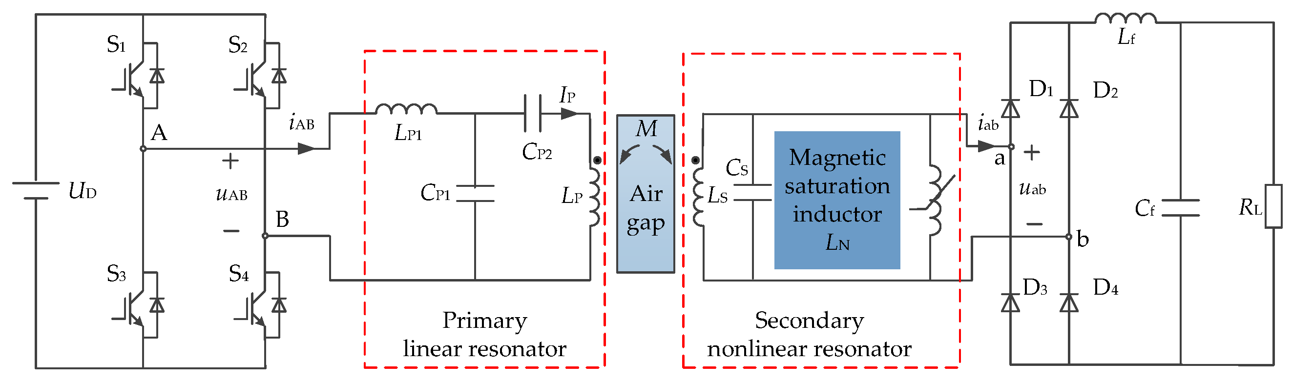
3.1. Nonlinear Topology

The nonlinear IPT system is shown in Figure 3, which is composed of a DC voltage source, high-frequency inverter, primary linear resonator, secondary nonlinear resonator, rectifier, LC filter and load. Here, $U_{\mathrm{D}}$ is the DC input voltage. S${}_1$–S${}_4$ are four switches, which form a high-frequency full bridge inverter, and $u_{\mathrm{AB}}$ and $i_{\mathrm{AB}}$ represent its instantaneous output voltage and current, respectively. $L_{\mathrm{P}}1$, $C_{\mathrm{P}}1$ and $C_{\mathrm{P}}1$ make up the LCC-compensated topology for the primary side. The capacitor $C_{\mathrm{S}}$ and saturable inductor $L_{\mathrm{N}}$ are connected in parallel to form a secondary compensation network. For convenience, the primary and secondary topologies are collectively referred to as $\mathrm{LCC}-\mathrm{P}-{\mathrm{L}}_{\mathrm{N}}$. M represents mutual inductance. D${}_1$–D${}_4$ are four diodes that constitute an uncontrolled rectifier bridge, and $u_{\mathrm{ab}}$ and $i_{\mathrm{ab}}$ are its instantaneous input voltage and current, respectively. The LC filter consists of an inductor $L_{\mathrm{f}}$ and capacitor $C_{\mathrm{f}}$. $R_{\mathrm{L}}$ represents the resistive load of the system.

The fundamental harmonic approximation (FHA) method is widely used to analyze IPT systems. Here, $U_{\mathrm{AB}}$, $I_{\mathrm{AB}}$, $U_{\mathrm{ab}}$ and $I_{\mathrm{ab}}$ are, respectively, the root mean square (RMS) values of $u_{\mathrm{AB}}$, $i_{\mathrm{AB}}$, $u_{\mathrm{ab}}$ and $i_{\mathrm{ab}}$. $I_{\mathrm{P}}$ and $I_{\mathrm{S}}$ are the RMS values of the current flowing through the primary and secondary coils, respectively. According to the equivalent conversion relationship of the high-frequency inverter and the uncontrolled rectifier bridge, Equation (4) can be obtained.

$$\left\{\begin{array}{c}{R}_{\mathrm{eq}}=\frac{{\pi }^2}{8}{R}_{\mathrm{L}}\hfill \\ U_{\mathrm{AB}}=\frac{2\sqrt{2}}{\pi }{U}_{\mathrm{D}}\hfill \end{array}\right.$$

(4)

where $U_{\mathrm{AB}}$ is the output voltage of the inverter, $R_{\mathrm{eq}}$ is equivalent to the rectifier bridge and the resistance load $R_{\mathrm{L}}$. According to Kirchhoff’s voltage and current laws, the FHA model of LCC topology for the primary side is established first, which can be described as

$$\left\{\begin{array}{c}(j\omega L_{\mathrm{P}1}+\frac{1}{j\omega C_{\mathrm{P}1}}){\dot{I}}_{\mathrm{AB}}-\frac{1}{j\omega C_{\mathrm{P}1}}{\dot{I}}_{\mathrm{P}}={\dot{U}}_{\mathrm{AB}}\hfill \\ {\dot{I}}_{\mathrm{P}}(\frac{1}{j\omega C_{\mathrm{P}2}}+j\omega L_{\mathrm{P}}+Z_{\mathrm{ref}})=({\dot{I}}_{\mathrm{AB}}-{\dot{I}}_{\mathrm{P}})\frac{1}{j\omega C_{\mathrm{P}1}}\hfill \end{array}\right..$$

(5)

where $Z_{\mathrm{ref}}$ is the reflective impedance of the secondary side, which satisfies the relation $Z_{\mathrm{ref}}=\frac{{\left(\omega M\right)}^2}{Z_S}$. Here, $\omega$ represents the power angular frequency, M represents the mutual inductance of the primary and secondary coils and $Z_{\mathrm{S}}$ is the secondary side’s impedance. It can be seen from the first part of Equation (5) that the current of the primary coil is independent of the reflective impedance when Equation (6) is satisfied, which means that the primary coil current is independent of the secondary side.

$${\omega }_0=2\pi f_0=\frac{1}{\sqrt{L_{\mathrm{P}1}{C}_{\mathrm{P}1}}}$$

(6)

When the angular frequency $\omega$ of the power supply is equal to the natural frequency ${\omega }_0$ of the system, the current of the primary coil can be expressed as

$$\begin{array}{c}\hfill {\dot{I}}_{\mathrm{P}}=-j\omega C_{\mathrm{P}1}{\dot{U}}_{\mathrm{AB}}=\frac{{\dot{U}}_{\mathrm{AB}}}{j\omega L_{\mathrm{P}1}}.\end{array}$$

(7)

Based on the analysis of the transmitter, it can be obtained that if the compensation network parameters are configured according to Equation (6), the transmitting coil current is independent of the secondary side. Therefore, the equivalent circuit of the receiver can be obtained, which is shown in Figure 4a. Here, $U_{\mathrm{OC}}$ is the induced voltage (open circuit voltage) of the secondary side, which satisfies the relation ${\dot{U}}_{\mathrm{OC}}=j\omega M{\dot{I}}_{\mathrm{P}}=\frac{M{\dot{U}}_{\mathrm{AB}}}{L_{\mathrm{P}1}}$. According to Norton’s theorem, the equivalent circuit represented by the current source can be obtained, which is shown in Figure 4b. Here, $I_{\mathrm{SC}}$ is the short circuit current of the secondary side, which satisfies the relation ${\dot{I}}_{\mathrm{SC}}=\frac{{\dot{U}}_{\mathrm{OC}}}{j\omega M{L}_{\mathrm{S}}}=\frac{M{\dot{U}}_{\mathrm{AB}}}{j\omega M{L}_{\mathrm{S}}{L}_{\mathrm{P}1}}$. As shown in Figure 4c, the capacitor value $C_{\mathrm{S}}$ can be divided into two parts, namely $C_{\mathrm{S}}1$ and $C_{\mathrm{S}}2$, which are used to resonate with $L_{\mathrm{S}}$ and $L_{\mathrm{N}}$, respectively. Furthermore, when $C_{\mathrm{S}}1$ and $L_{\mathrm{S}}$ resonate at power frequency, the equivalent circuit can be simplified as Figure 4d. Next, the nonlinear resonator shown in Figure 4d will be analyzed and discussed.

3.2. Saturable Inductor Modeling

In order to study the new topology, it is necessary to research the saturation phenomenon of the inductor. This part attempts to derive the inductance values in the linear state and nonlinear state; the detailed analysis of inductor $L_{\mathrm{N}}$ is applied as follows

$$\begin{array}{c}\hfill L=\frac{\lambda }{i}.\end{array}$$

(8)

where $\lambda =N\varphi$ represents the flux linkage, N is the winding numbers, $\varphi$ denotes the magnetic flux and i is the current flowing through the inductor. When the current flowing through the saturable inductor does not exceed its saturation current, it works in a linear state and its inductance value is the maximum, i.e., $L_{\max }$, which satisfies the following formula:

$$\begin{array}{c}\hfill L_{max}=\frac{{\mu }_0{\mu }_{\mathrm{r}}{N}^{2}S}{l}.\end{array}$$

(9)

where S represents the cross-sectional area, l represents the circumference of the magnetic core, ${\mu }_0=4\pi {10}^{-7}N{A}^{-2}$ represents the vacuum permeability and ${\mu }_{\mathrm{r}}$ represents the relative permeability. If the current flowing through the inductor is large, the magnetic flux linkage is no longer a linear function of current and can be expressed as

$$\begin{array}{c}\hfill \lambda =\psi \left(i\right)=N\phi .\end{array}$$

(10)

In particular, when the current flowing through the inductor is a sine wave, i.e., $i\left(t\right)=I_{\mathrm{peak}}sin\left(\omega t\right)$. Where $I_{\mathrm{peak}}$ is the amplitude of the current and $\omega =2\pi f$ represents the angular frequency of the current. Based on the definition of Equations (8) and (10) and the describing function definition in Equation (A7) (As shown in Appendix A) [31,32], the saturable inductor’s equivalent inductance $L_{\mathrm{eff}}$ can be derived as

$$\begin{array}{c}\hfill L_{\mathrm{eff}}=N(I_{\mathrm{peak}},\omega )=\frac{j}{I_{\mathrm{peak}}\pi }\underset{-\pi }{\overset{\pi }{\int }}\psi (I_{\mathrm{peak}}sin\omega t)e^{-j\omega t}d\left(\omega t\right).\end{array}$$

(11)

In general, the magnetic flux will be saturated if the current flowing through the inductor is high enough. Therefore, the saturation characteristic can be expressed as

$$\psi \left(i\right)=sat\left(i\right)=\left\{\begin{array}{c}{L}_{max}{I}_{\mathrm{sat}},i>I_{\mathrm{sat}}\hfill \\ L_{max}i,I_{\mathrm{sat}}\ge i\ge -I_{\mathrm{sat}}\hfill \\ -L_{max}{I}_{\mathrm{sat}},i<I_{\mathrm{sat}}\hfill \end{array}\right.$$

(12)

where $I_{\mathrm{sat}}$ represents the saturation current, and $L_{\max }$ represents the inductance in the linear state, as shown in Figure 5. The lower-right corner of Figure 5 is the saturable inductor proposed in this paper. Furthermore, based on Equations (11) and (12), the saturable inductor’s equivalent inductance $L_{\mathrm{eff}}$ can be obtained by

$$\begin{array}{c}\hfill L_{\mathrm{eff}}=\frac{2L_{max}}{\pi }\left[{sin}^{-1}\frac{I_{\mathrm{sat}}}{I_{\mathrm{peak}}}+\frac{I_{\mathrm{sat}}}{I_{\mathrm{peak}}}\sqrt{1-{\left(\frac{I_{\mathrm{sat}}}{I_{\mathrm{peak}}}\right)}^2}\right].\end{array}$$

(13)

where the saturation current $I_{\mathrm{sat}}$ of the saturable inductor can be written as

$$\begin{array}{c}\hfill I_{\mathrm{sat}}=\frac{B_{\mathrm{sat}}{l}_{\mathrm{m}}}{\mu {\mu }_{0}N}.\end{array}$$

(14)

It should be noted that $I_{\mathrm{peak}}$ is the amplitude of the AC current flowing through the saturable inductor, and $I_{\mathrm{sat}}$ is the amplitude of the saturation current. However, RMS values can be used when calculating the ratio $\frac{I_{\mathrm{sat}}}{I_{\mathrm{peak}}}$. When $\frac{I_{\mathrm{peak}}}{I_{\mathrm{sat}}}>3$, the second term in Equation (13) can be ignored, which can be simplified as

$$\begin{array}{c}\hfill L_{\mathrm{eff}}=\frac{2L_{max}}{\pi }\left[{sin}^{-1}\frac{I_{\mathrm{sat}}}{I_{\mathrm{peak}}}\right].\end{array}$$

(15)

According tothe Taylor series, the first term can be further simplified, the equivalent inductance $L_{\mathrm{eff}}$ can be described as

$$\begin{array}{c}\hfill L_{\mathrm{eff}}=\frac{4L_{max}}{\pi }\left[\frac{I_{\mathrm{sat}}}{I_{\mathrm{peak}}}\right].\end{array}$$

(16)

Therefore, Equations (9), (13), (15) and (16) are used to calculate the inductance of the saturable inductor with different sine wave AC excitation, which is shown in Figure 6. It can be seen that the equivalent inductance decreases with the increase in the excitation current, and the error among the three simplified models decreases with the increase in the excitation current. By combining Equations (9) and (16), the saturable inductor’s effective inductance working in saturated and unsaturated conditions can be described as

$$L_{\mathrm{eff}}=\left\{\begin{array}{c}{L}_{\max },i_{\mathrm{sat}}>I_{\mathrm{peak}}\hfill \\ \frac{4L_{\max }}{\pi }\left(\frac{I_{\mathrm{sat}}}{I_{\mathrm{peak}}}\right),i_{\mathrm{sat}}\le I_{\mathrm{peak}}\hfill \end{array}\right.$$

(17)

Based on the above analysis, the equivalent inductance is closely related to the excitation current amplitude when the power frequency is kept constant. Since the current is a sine wave, Equation $L_{\mathrm{eff}}\left(I_{\mathrm{peak}}\right)=L_{\mathrm{eff}}(-I_{\mathrm{peak}})$ must be satisfied, which is the basis of the following analysis. The magnetic ring with N turn coils can be selected to provide the saturable characteristics. As shown in Figure 5, the TDK PC95 ring is selected for the saturable inductor, with an outer diameter of 25 mm, an inner diameter of 15 mm and a height of 13 mm. The number of coil turns is 16. In the practice application, the two saturable inductors can be connected in series to increase the output voltage. The role of the saturable inductor in the IPT system is analyzed as follows.

3.3. Effect of Saturable Inductor on System Performance

The voltage across the saturated inductor satisfies the relation $u=d\psi /dt$, where $\psi$ represents the magnetic flux. According to Kirchhoff’s current law (KCL), the time-domain dynamic equation describing the behavior of the nonlinear parallel RLC resonant circuit (as shown in Figure 4d) can be written as

$$\begin{array}{c}\hfill i_{\mathrm{LN}}+\frac{1}{R_{\mathrm{L}}}\frac{d{\psi }_{\mathrm{LN}}}{dt}+C_{\mathrm{S}2}\frac{d{\psi }_{{}_{\mathrm{LN}}}^2}{d{t}^2}=i_{\mathrm{SC}}.\end{array}$$

(18)

where $i_{\mathrm{SC}}=I_{\mathrm{SC}-\mathrm{peak}}cos\left(\omega t\right)$ is the excitation current and $i_{\mathrm{LN}}$ is the current of the saturable inductor. ${\psi }_{\mathrm{LN}}\left(t\right)$ is the amount of the magnetic flux that is stored in the saturable inductor. The fundamental relationship of current $i_{\mathrm{LN}}$, voltage $u_{\mathrm{LN}}$ and magnetic flux ${\psi }_{\mathrm{LN}}\left(t\right)$ of a saturable inductor is described as follows:

$$\begin{array}{c}\hfill d{\psi }_{\mathrm{LN}}=L_{\mathrm{N}}d{i}_{\mathrm{LN}}+i_{\mathrm{LN}}d{L}_{\mathrm{N}}.\end{array}$$

(19)

Therefore, the total magnetic flux stored in a cycle can be described as

$$\begin{array}{c}\hfill {\psi }_{\mathrm{LN}}=\int (L_{\mathrm{N}}d{i}_{\mathrm{LN}}+i_{\mathrm{LN}}d{L}_{\mathrm{N}})=\int (L_{\mathrm{N}}+i_{\mathrm{LN}}\frac{d{L}_{\mathrm{N}}}{d{i}_{\mathrm{LN}}})d{i}_{\mathrm{LN}}.\end{array}$$

(20)

The $L_{\mathrm{N}}-i_{\mathrm{LN}}$ relationship of a saturable inductor can be approximately depicted by the n-order Taylor polynomial. Since it is centrosymmetric, the even-order term can be used to describe the nonlinearity of the saturable inductor.

$$\begin{array}{c}\hfill L_{\mathrm{N}}=L_0+L_2{i}_{{}_{\mathrm{LN}}}^2+L_4{i}_{{}_{\mathrm{LN}}}^4+L_6{i}_{{}_{\mathrm{LN}}}^6+···+L_{\mathrm{n}}{i}_{{}_{\mathrm{LN}}}^{\mathrm{n}}.\end{array}$$

(21)

By substituting Equation (21) into Equation (20), ${\psi }_{{}_{\mathrm{LN}}}$ can be written as

$$\begin{array}{c}\hfill {\psi }_{\mathrm{LN}}=\int \sum _{i=0}^{\mathrm{n}\left(\mathrm{even}\right)}(i+1)L_{\mathrm{i}}{i}_{{}_{\mathrm{LN}}}^{\mathrm{i}}d{i}_{\mathrm{LN}}=\sum _{i=0}^{\mathrm{n}\left(\mathrm{even}\right)}{L}_{\mathrm{i}}{i}_{{}_{\mathrm{LN}}}^{\mathrm{i}+1}.\end{array}$$

(22)

where ${\psi }_{{}_{\mathrm{LN}}}$ is an odd function of $i_{\mathrm{LN}}$. Therefore, $i_{\mathrm{LN}}$ can be expressed by ${\psi }_{{}_{\mathrm{LN}}}$ using the inverse Taylor expansion. When the terms that are higher than third-order are neglected, the current $i_{\mathrm{LN}}$ flowing through the saturable inductor can be described as

$$\begin{array}{c}\hfill i_{\mathrm{LN}}=\frac{1}{{a_1}^{\prime }}{\psi }_{\mathrm{LN}}+\frac{1}{{a_3}^{\prime }}{\psi }_{{}_{\mathrm{LN}}}^3.\end{array}$$

(23)

In general, ${a_1}^{\prime }$ and ${a_3}^{\prime }$ can be approximated by the $L_{\mathrm{N}}-i_{\mathrm{LN}}$ relationship of the saturable inductor. Combining (23) and (18), the following equation can be obtained.

$$\begin{array}{c}\hfill \frac{d{\psi }_{{}_{\mathrm{LN}}}^2}{dt}+\frac{1}{R_{\mathrm{L}}{C}_{\mathrm{S}2}}\frac{d{\psi }_{\mathrm{LN}}}{dt}+\frac{1}{{a_1}^{\prime }{C}_{\mathrm{S}2}}{\psi }_{\mathrm{LN}}+\frac{1}{{a_3}^{\prime }{C}_{\mathrm{S}2}}{\psi }_{{}_{\mathrm{LN}}}^3=\frac{I_{\mathrm{SC}-\mathrm{peak}}}{C_{\mathrm{S}2}}cos\left(\omega t\right)\end{array}$$

(24)

Equation (24) has the same mathematical form as the Duffing equation, which is depicted in (1). It should be noted that if the five-order term of the $L_{\mathrm{N}}-i_{\mathrm{LN}}$ relationship is not ignored, the Duffing equation with a five-order term will be obtained. Similarly, if the five-order term and seven-order term are not ignored, the Duffing equation with a seven-order term will be obtained, and so on, the solution will be more and more accurate. The solution of Equation (24) can be written as ${\psi }_{\mathrm{LN}}\left(t\right)={\psi }_{\mathrm{m}}cos(\omega t-\theta )$. Where ${\psi }_{\mathrm{m}}$ is the maximum amount of magnetic flux that is stored in the saturable inductor in a period. $\theta$ is the phase shift in relation to excitation source.

The restoring force is composed of a linear part ${\psi }_{\mathrm{LN}}\left(t\right)/{a_1}^{\prime }{C}_{\mathrm{S}2}$ and a nonlinear part ${\psi }_{{}_{\mathrm{LN}}}^3/{a_3}^{\prime }{C}_{\mathrm{S}2}$. For simplified analysis, the equivalent inductance ${L_3}^{\prime }$ is defined to quantify the restoring force, which is contributed by the nonlinear part based on the law of energy conservation, which can be written as

$$\begin{array}{c}\hfill {\int }_0^{\frac{T}{4}}\frac{d\left(\frac{1}{{L_3}^{\prime }{C}_{\mathrm{S}2}}{\psi }_{\mathrm{LN}}\right)}{dt}\frac{\frac{1}{{L_3}^{\prime }{C}_{\mathrm{S}2}}{\psi }_{\mathrm{LN}}}{{L_3}^{\prime }}dt={\int }_0^{\frac{T}{4}}\frac{d\left(\frac{1}{a_3{C}_{\mathrm{S}2}}{\psi }_{{}_{\mathrm{LN}}}^3\right)}{dt}\frac{\frac{1}{a_3{C}_{\mathrm{S}2}}{\psi }_{{}_{\mathrm{LN}}}^3}{{L_3}^{\prime }}dt.\end{array}$$

(25)

Based on (25), ${L_3}^{\prime }$ can be written as

$$\begin{array}{c}\hfill {L_3}^{\prime }=\frac{a_3}{{\psi }_{\mathrm{m}}^2}.\end{array}$$

(26)

In nonlinear systems, the nonlinear terms do not operate throughout the period, so ${L_3}^{\prime }$ should be multiplied by a coefficient greater than 1. However, the qualitative analysis of the system is not affected. The simplified equivalent inductance ${L_{\mathrm{eff}}}^{\prime }$ can be written as

$$\begin{array}{c}\hfill {L_{\mathrm{eff}}}^{\prime }=\frac{1}{{L_1}^{\prime }}+\frac{1}{{L_3}^{\prime }}.\end{array}$$

(27)

where ${L_{\mathrm{eff}}}^{\prime }$ is the simplification of $L_{\mathrm{eff}}$ (As shown in Equations (13), (15) and (16)), i.e., the five-order term and the terms higher than five-order are ignored. Therefore, the natural angular frequency ${\omega }_0$ of the nonlinear resonator can be obtained from

$$\begin{array}{c}\hfill {\omega }_0=\sqrt{\frac{1}{C_{\mathrm{S}2}}\frac{1}{{L_{\mathrm{eff}}}^{\prime }}}=\sqrt{\frac{1}{C_{\mathrm{S}2}}(\frac{1}{{L_1}^{\prime }}+\frac{1}{{L_3}^{\prime }})}.\end{array}$$

(28)

Substituting (27) into (24), Equation (29) can be obtained.

$$\begin{array}{c}\hfill \frac{d{\psi }_{{}_{\mathrm{LN}}}^2}{dt}+\frac{1}{R_{\mathrm{L}}{C}_{\mathrm{S}2}}\frac{d{\psi }_{\mathrm{LN}}}{dt}+(\frac{1}{a_1{C}_{\mathrm{S}2}}+\frac{1}{{L_3}^{\prime }{C}_{\mathrm{S}2}}){\psi }_{\mathrm{LN}}=\frac{I_{\mathrm{SC}-\mathrm{peak}}}{C_{\mathrm{S}2}}cos\left(\omega t\right)\end{array}$$

(29)

Furthermore, the differential equation can be transformed into the frequency domain form, which can be written as

$$\begin{array}{c}\hfill {\left(j\omega \right)}^{2}Z+\left(j\omega \right)\frac{1}{R_{\mathrm{L}}{C}_{\mathrm{S}2}}Z+(\frac{1}{a_1{C}_{\mathrm{S}2}}+\frac{1}{{L_3}^{\prime }{C}_{\mathrm{S}2}})Z=\frac{I_{\mathrm{SC}-\mathrm{peak}}}{C_{\mathrm{S}2}}.\end{array}$$

(30)

where $Z={\psi }_{\mathrm{m}}{e}^{-j\theta }$ is the phasor form of ${\psi }_{\mathrm{LN}}$. At last, combining (26) and (30), Equation (31) can be obtained.

$$\begin{array}{c}\hfill {\psi }_{\mathrm{m}}^2{({\omega }_0^2-{\omega }^2)}^2+{\left(\frac{1}{R_{\mathrm{L}}{C}_{\mathrm{S}2}}{\psi }_{\mathrm{m}}\omega \right)}^2={\left(\frac{I_{\mathrm{SC}-\mathrm{peak}}}{C_{\mathrm{S}2}}\right)}^2\end{array}$$

(31)

Therefore, the maximum amount of magnetic flux ${\psi }_{\mathrm{m}}$ can be achieved, which is a function of power angular frequency $\omega$ and excitation amplitude $I_{\mathrm{SC}-\mathrm{peak}}$. Then, the voltage across the saturable inductor is determined by

$$\begin{array}{c}\hfill U_{\mathrm{LN}}=\frac{d{\psi }_{\mathrm{LN}}\left(t\right)}{dt}=4.44fN{\psi }_{\mathrm{m}}.\end{array}$$

(32)

Based on the above analysis, it can be concluded that the nonlinear resonator can be constructed by using the magnetic saturation inductor and linear capacitor, which can be simplified and described by the Duffing equation. If the higher-order term is not neglected, the nonlinear resonator can be described by the Duffing equation with higher terms. The IPT system with a nonlinear resonator has hysteresis and hopping characteristics. The equivalent inductance ${L_{\mathrm{eff}}}^{\prime }$ is negatively related to the excitation amplitude and excitation frequency. The IPT system with a nonlinear resonator has a negative feedback function, which reduces the fluctuation in the output voltage. When the IPT system with a saturable inductor works in a nonlinear state, the magnetic flux ${\psi }_{\mathrm{m}}$ stays basically unchanged even if the amplitude and frequency of the excitation current varies within a certain range, so the output voltage $U_{\mathrm{LN}}$ can be basically maintained. In addition, the output voltage of an IPT system with a saturable inductor can be adjusted by changing the magnetic material, the size of the magnetic ring, the number of coil turns and the wire winding method.

4. Experimental Validation and Further Discussion

In order to prove the correctness of the IPT system employing a nonlinear resonator, an experimental prototype with an output voltage of about 140 V is designed, as shown in Figure 7. It is composed of IT6523D DC power supply, TMS320F28335 controller, high-frequency inverter, loosely coupled transformer, $\mathrm{LCC}-\mathrm{P}-{\mathrm{L}}_{\mathrm{N}}$ compensation network, uncontrolled rectifier, MAYNUO M9715B electronic load, RIGOL DS1074 oscilloscope, HIOKI PW6001 power analyzer, etc. The DD (double D) coil is simple in structure and can effectively improve the height of the magnetic field and the central magnetic flux of transmitting and receiving coils. Therefore, the DD coil is used as the magnetic coupling mechanism in this paper. It should be noted that any coil structure is suitable for the designed nonlinear IPT system. By choosing the appropriate magnetic material and magnetic ring size, different types of saturable inductors can be designed, and IPT systems with different voltage levels and operating frequencies can be achieved. Two TDK PC95 ring with 16 turns (As shown in Figure 5) are connected in series to ensure that the output voltage of the IPT system is approximately 140 V. The other parameters, including $L_{\mathrm{P}}$, $L_{\mathrm{S}}$, $L_{\mathrm{P}}1$, $C_{\mathrm{P}}1$, $C_{\mathrm{P}}2$, $C_{\mathrm{S}}$, f, $L_{\mathrm{f}}$ and $C_{\mathrm{f}}$, are listed in

Table 1. Parameters of the experimental prototype.

Symbol	Note	Values
$L_{\mathrm{P}}$	Primary-side coil inductance	$112\mathsf{\mu H}$
$L_{\mathrm{S}}$	Secondary-side coil inductance	$112\mathsf{\mu H}$
$L_{\mathrm{P}1}$	Inductance of primary compensation network	$56\mathsf{\mu H}$
$C_{\mathrm{P}1}$	Shunt capacitance of primary compensation network	$0.47\mathsf{\mu F}$
$C_{\mathrm{P}2}$	Series capacitance of primary Compensation network	$0.47\mathsf{\mu F}$
$C_{\mathrm{S}}$	Secondary Compensation network capacitance	$0.34\mathsf{\mu F}$
f	Optimum operating frequency in linear state	$\sim 31\mathrm{kHz}$
$L_{\mathrm{f}}$	Filter inductor	$60\mathsf{\mu H}$
$C_{\mathrm{f}}$	Filter capacitor	$110\mathsf{\mu F}$

.

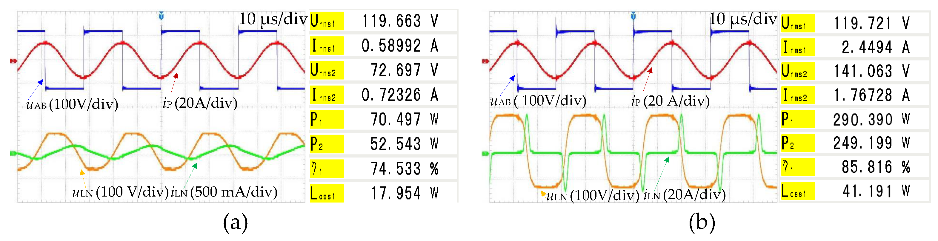
4.1. Waveforms Analysis of the IPT System

The experimental waveforms and measured results of the IPT system working in linear and nonlinear states are shown in Figure 8a,b, respectively. In these waveforms, $u_{\mathrm{AB}}$ is the output voltage of the inverter, $i_{\mathrm{P}}$ is the current flowing through the transmitting coil, $u_{\mathrm{LN}}$ is the voltage across the saturable inductor, and $i_{\mathrm{LN}}$ is the current flowing through the saturable inductor. Among the measured items, $U_{\mathrm{rms}}1$ and $I_{\mathrm{rms}}1$ represent input DC voltage and current and $U_{\mathrm{rms}}2$ and $I_{\mathrm{rms}}2$ represent output DC voltage and current. $P_1$ and $P_2$ are input and output power, respectively, and ${\eta }_1$ and $L_{\mathrm{oss}}1$ are the efficiency and losses, respectively. As shown in Figure 8a), the IPT system works in a linear state when $k=0.18$. The current $i_{\mathrm{LN}}$ flowing through the saturable inductor is close to a sine wave, and the voltage across the saturable inductor is also relatively small. As shown in Figure 8b, the IPT system works in a nonlinear state when $k=0.27$. The current $i_{\mathrm{LN}}$ varies dramatically, and its waveform is not a sine wave. At the same time, the voltage waveform is close to a flat-top wave, and the voltage RMS value is almost twice that of the linear state. The sharp change in the current flowing through a saturable inductor will cause electromagnetic interference to the IPT system. Therefore, the magnetic flux of the magnetic coupler should be guided and shielded by a high-permeability ferrite core and aluminum plate, respectively, in the actual nonlinear IPT system.

The reason for such behavior is that when $k=0.18$, the current flowing through the saturable inductor is small and satisfies $i_{\mathrm{LN}-\mathrm{peak}}<I_{\mathrm{sat}}$; the inductor is not saturated. The inductance value of the saturable inductor is larger than that of the receiving coil, so the saturable inductor branch is close to the open state. When $k=0.27$, the current flowing through the saturable inductor is large enough to meet $i_{\mathrm{LN}-\mathrm{peak}}>I_{\mathrm{sat}}$, the inductor goes into a nonlinear state, the inductance value decreases and the current flowing through the saturable inductor varies dramatically. Therefore, the transformation of the nonlinear resonator from the linear state to the nonlinear state requires certain excitation conditions, which may be the excitation amplitude or the excitation frequency.

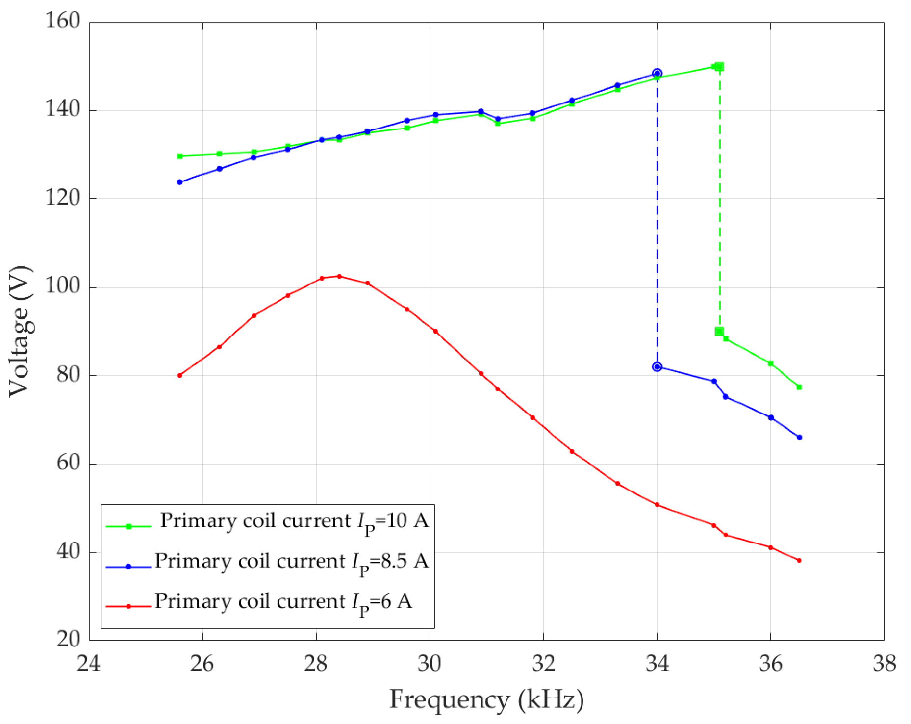
4.2. Hysteresis and Jumping Characteristics

The output voltage with respect to power frequency is measured when $I_{\mathrm{P}}=10\mathrm{A}$ and $R_{\mathrm{L}}=80\mathrm{\Omega }$, which is shown in Figure 9. When the power frequency is varied continuously from $25.6$ to $35.1\mathrm{kHz}$ (boundary frequency), the output voltage varies along the upper curve, the IPT system operate in nonlinear state. When the power frequency reaches $35.1\mathrm{kHz}$, the working point of the IPT system jumps from point 1 to point 2, and the output voltage drops rapidly. If the power frequency is continuously increased, the output voltage decreases along the bottom curve. On the contrary, if the power frequency decreases, the output voltage increases along the bottom curve. When the power frequency decreases to $32.5\mathrm{kHz}$ (boundary frequency), the system jumps from point 3 to point 4, and the output voltage jumps to about 140 V. If the power frequency is continuously decreased, the output voltage varies along the top curve. The experimental results show that the IPT system proposed in this paper has a jumping characteristic, which is not possessed by traditional IPT systems.

As shown in Figure 10, the output voltage with respect to power frequency is measured when $I_{\mathrm{P}}=6$, 8.5 and $10\mathrm{A}$, respectively. When $I_{\mathrm{P}}=6\mathrm{A}$, the system always works in the linear state. When $I_{\mathrm{P}}=8.5\mathrm{A}$, $I_{\mathrm{P}}=10\mathrm{A}$ and the power frequency is less than the jumping frequency, the system works in the nonlinear state. It should be noted that the bandwidth ($25.6$–$35\mathrm{kHz}$) corresponding to $I_{\mathrm{P}}=10\mathrm{A}$ is 1.7 times than that (25.6–31.2 kHz) corresponding to $I_{\mathrm{P}}=6\mathrm{A}$. Here, the bandwidth is defined as the frequency range in which the output voltage is larger than $1/\sqrt{2}$ of its maximum value. The experimental results show that the IPT system proposed in this paper has a hysteresis characteristic that is not possessed by traditional IPT systems. Therefore, the proposed system can achieve relatively stable output voltage in a wide frequency range.

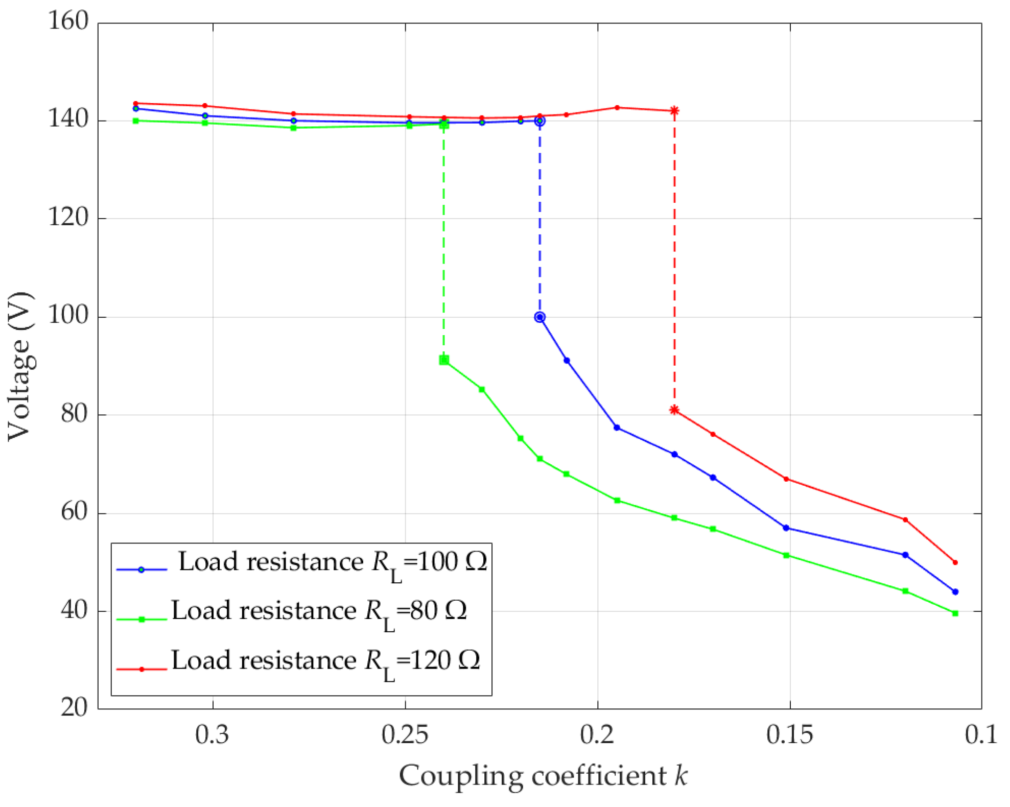
4.3. Position and Load Insensitivity

As shown in Figure 11, the output voltage with respect to coupling coefficient k are measured when $R_{\mathrm{L}}=80$, 100 and $120\mathrm{\Omega }$, respectively. Here, the output voltage ripple is defined as $\mathrm{VR}=\frac{U_{\mathrm{RL}-\max }-U_{\mathrm{RL}-\min }}{U_{\mathrm{RL}-\max }+U_{\mathrm{RL}-\min }}\times 100\%$. When $R_{\mathrm{L}}=80\mathrm{\Omega }$, and the coupling coefficient varies from 0.32 to 0.24, the IPT system operates in the nonlinear state with a maximum output voltage of $140.0\mathrm{V}$ and a minimum output voltage of $138.6\mathrm{V}$. When $R_{\mathrm{L}}=100\mathrm{\Omega }$, and the coupling coefficient ranges from 0.32 to 0.215, the IPT system operates in the nonlinear state with a maximum output voltage of $142.5\mathrm{V}$ and a minimum output voltage of $139.7\mathrm{V}$. Similarly, when $R_{\mathrm{L}}=120\mathrm{\Omega }$, and the coupling coefficient varies from 0.32 to 0.18, the IPT system operates in the nonlinear state with a maximum output voltage of $143.6\mathrm{V}$ and a minimum output voltage of $140.6\mathrm{V}$. In summary, when the coupling coefficient varies from 0.32 to 0.24 and the load resistance varies from 80 to $120\mathrm{\Omega }$, the system works in a nonlinear state and the output voltage ripple is 1.77%. The above results show that as long as the proposed IPT system operates in the nonlinear resonant state, the RMS value of the output voltage is basically unchanged. In addition, the corresponding boundary coupling coefficient decreases with the increase in load resistance. Because the reduction in the coupling coefficient means that the excitation amplitude decreases, indicating that the larger the load is, the larger the required excitation amplitude is.

It can be seen from Figure 12 that the DC-DC efficiency with respect to coupling coefficient k is measured when $R_{\mathrm{L}}=80$, 100 and $120\mathrm{\Omega }$, respectively. When the IPT system with $R_{\mathrm{L}}=80\mathrm{\Omega }$ works in the nonlinear resonance state, the overall efficiency is not less than 87.2%. When the IPT system with $R_{\mathrm{L}}=100\mathrm{\Omega }$ works in the nonlinear resonance state, the overall efficiency is not less than 85.2%. When the IPT system with $R_{\mathrm{L}}=120\mathrm{\Omega }$ works in the nonlinear resonance state, the overall efficiency is not less than 82.6%. In summary, the DC-DC efficiency of the IPT system working in the nonlinear state is not less than 82.6%. The DC-DC efficiency of the IPT system in the nonlinear state is much higher than that in the linear state, and the IPT system can work with high efficiency in a large range. When the IPT system operates in the nonlinear resonant state, the saturable inductor participates in the resonance, the temperature of the saturable inductor rises due to its material characteristics and the system losses may be increased. The saturable inductor losses consist of copper loss and iron loss, which are closely related to the magnetic materials, output power, operating frequency and temperature. Therefore, the losses in the system can be further reduced by selecting suitable magnetic materials and appropriate cooling measures. In addition, the losses of the inverter, rectifier and other switching components can be reduced by a reasonable switch selection scheme, which is beyond the scope of this paper.

5. Conclusions

This paper proposes a novel nonlinear IPT system with a saturable inductor, which is independent of the coupling coefficients and load resistances. A IPT system prototype with an output voltage of approximately $140\mathrm{V}$ is designed, implemented and measured. The experimental results show that when the nonlinear IPT system works in the nonlinear resonant state, the output voltage ripple is only 1.77%, and the DC-DC efficiency is higher than 82.60%. The experimental results agree with the theoretical analysis, indicating that the proposed system has a strong anti-misalignment ability. It should be noted that the saturable inductor proposed in this paper can be used to construct the nonlinear IPT system with different compensation topologies. The nonlinear IPT system does not require any detection circuit and control strategy and has the advantages of simple structure, low cost and strong robustness. It is suitable for the application scenarios of constant voltage charging, such as electronic equipment and electric vehicles.

References

1. Aydin, E.; Aydemir, M.T.; Aksoz, A.; El Baghdadi, M.; Hegazy, O. Inductive Power Transfer for Electric Vehicle Charging Applications: A Comprehensive Review. Energies 2022, 15, 4962. [Google Scholar] [CrossRef]
2. Yuan, Z.; Yang, Q.; Zhang, X.; Ma, X.; Chen, Z.; Xue, M.; Zhang, P. High-Order Compensation Topology Integration for High-Tolerant Wireless Power Transfer. Energies 2023, 16, 638. [Google Scholar] [CrossRef]
3. El Ghanam, E.; Hassan, M.; Osman, A. Design of a High Power, LCC-Compensated, Dynamic, Wireless Electric Vehicle Charging System with Improved Misalignment Tolerance. Energies 2021, 14, 885. [Google Scholar] [CrossRef]
4. Budhia, M.; Boys, J.T.; Covic, G.A.; Huang, C.-Y. Development of a Single-Sided Flux Magnetic Coupler for Electric Vehicle IPT Charging Systems. IEEE Trans. Power Electron. 2013, 60, 318–328. [Google Scholar] [CrossRef]
5. Zaheer, A.; Covic, G.A.; Kacprzak, D. A Bipolar Pad in a 10-kHz 300-W Distributed IPT System for AGV Applications. IEEE Trans. Ind. Electron. 2014, 61, 3288–3301. [Google Scholar] [CrossRef]
6. Kim, S.; Covic, G.A.; Boys, J.T. Tripolar Pad for Inductive Power Transfer Systems for EV Charging. IEEE Trans. Power Electron. 2017, 32, 5045–5057. [Google Scholar] [CrossRef]
7. Yang, X.; Yang, J.; Fan, J.; Wang, B.; Li, D. A Magnetic Field Containment Method for an IPT System with Multiple Transmitting Coils Based on Reflective Properties. Electronics 2023, 12, 653. [Google Scholar] [CrossRef]
8. Chen, C.; Zhou, H.; Deng, Q.; Hu, W.; Yu, Y.; Lu, X.; Lai, J. Modeling and Decoupled Control of Inductive Power Transfer to Implement Constant Current/Voltage Charging and ZVS Operating for Electric Vehicles. IEEE Access. 2018, 6, 59917–59928. [Google Scholar] [CrossRef]
9. Joseph, P.K.; Elangovan, D.; Arunkumar, G. Linear control of wireless charging for electric bicycles. Appl. Energy 2019, 255, 113898. [Google Scholar] [CrossRef]
10. Colak, K.; Asa, E.; Bojarski, M.; Czarkowski, D.; Onar, O.C. A Novel Phase-Shift Control of Semibridgeless Active Rectifier for Wireless Power Transfer. IEEE Trans. Power Electron. 2015, 30, 6288–6297. [Google Scholar] [CrossRef]
11. Lee, J.H.; Son, W.-J.; Ann, S.; Byun, J.; Lee, B.K. Improved Pulse Density Modulation with a Distribution Algorithm for Semi-Bridgeless Rectifier of Inductive Power Transfer System in Electric Vehicles. In Proceedings of the 2019 10th International Conference on Power Electronics and ECCE Asia—ICPE 2019—ECCE Asia, Busan, Republic of Korea, 27–30 May 2019; pp. 1–6. [Google Scholar]
12. Diekhans, T.; Doncker, R.W.D. A Dual-Side Controlled Inductive Power Transfer System Optimized for Large Coupling Factor Variations and Partial Load. IEEE Trans. Power Electron. 2015, 30, 6320–6328. [Google Scholar] [CrossRef]
13. Zhong, W.; Hui, S.Y.R. Charging Time Control of Wireless Power Transfer Systems Without Using Mutual Coupling Information and Wireless Communication System. IEEE Trans. Ind. Electron. 2017, 64, 228–235. [Google Scholar] [CrossRef]
14. Feng, H.; Cai, T.; Duan, S.; Zhao, J.; Zhang, X.; Chen, C. An LCC-Compensated Resonant Converter Optimized for Robust Reaction to Large Coupling Variation in Dynamic Wireless Power Transfer. IEEE Trans. Ind. Electron. 2016, 63, 6591–6601. [Google Scholar] [CrossRef]
15. Borage, M.; Tiwari, S.; Kotaiah, S. Analysis and design of an LCL-T resonant converter as a constant-current power supply. IEEE Trans. Ind. Electron. 2005, 52, 1547–1554. [Google Scholar] [CrossRef]
16. Zhao, L.; Thrimawithana, D.J.; Madawala, U.K. Hybrid Bidirectional Wireless EV Charging System Tolerant to Pad Misalignment. IEEE Trans. Ind. Electron. 2017, 64, 7079–7086. [Google Scholar] [CrossRef]
17. Villa, J.L.; Sallan, J.; Osorio, J.F.S.; Llombart, A. High-Misalignment Tolerant Compensation Topology For ICPT Systems. IEEE Trans. Ind. Electron. 2012, 59, 945–951. [Google Scholar] [CrossRef]
18. Aldhaher, S.; Luk, P.C.-K.; Bati, A.; Whidborne, J.F. Wireless Power Transfer Using Class E Inverter With Saturable DC-Feed Inductor. IEEE T. Ind. Appl. 2014, 50, 2710–2718. [Google Scholar] [CrossRef] [Green Version]
19. Mai, R.; Chen, Y.; Li, Y.; Zhang, Y.; Cao, G.; He, Z. Inductive Power Transfer for Massive Electric Bicycles Charging Based on Hybrid Topology Switching With a Single Inverter. IEEE Trans. Power Electron. 2017, 32, 5897–5906. [Google Scholar] [CrossRef]
20. Wang, X.; Mortazawi, A. Bandwidth Enhancement of RF Resonators Using Duffing Nonlinear Resonance for Wireless Power Applications. IEEE Trans. Microw. Theory Tech. 2016, 64, 3695–3702. [Google Scholar] [CrossRef]
21. Abdelatty, O.; Wang, X.; Mortazawi, A. Position-Insensitive Wireless Power Transfer Based on Nonlinear Resonant Circuits. IEEE Trans. Microw. Theory Tech. 2019, 67, 3844–3855. [Google Scholar] [CrossRef]
22. Chai, R.; Mortazawi, A. A Position-Insensitive Wireless Power Transfer System Employing Coupled Nonlinear Resonators. IEEE Trans. Microw. Theory Tech. 2021, 69, 1752–1759. [Google Scholar] [CrossRef]
23. Zhou, J.; Zhang, B.; Liu, G.; Qiu, D. Resonance and Distance Insensitive Wireless Power. Transfer with Parity-Time Symmetric Duffing Resonators. In Proceedings of the 2018 IEEE Wireless Power Transfer Conference (WPTC), Montreal, QC, Canada, 3–7 June 2018; pp. 1–4. [Google Scholar]
24. Zhou, J.; Zhang, B.; Xiao, W.; Qiu, D.; Chen, Y. Nonlinear Parity-Time-Symmetric Model for Constant Efficiency Wireless Power Transfer: Application to a Drone-in-Flight Wireless Charging Platform. IEEE Trans. Ind. Electron. 2019, 66, 4097–4107. [Google Scholar] [CrossRef]
25. Wu, L.; Zhang, B.; Jiang, Y.; Zhou, J. A Robust Parity-Time-Symmetric WPT System With Extended Constant-Power Range for Cordless Kitchen Appliances. IEEE Trans. Ind. Electron. 2012, 58, 1179–1189. [Google Scholar] [CrossRef]
26. Yang, X.; Jiao, C.; Yang, J.; Fan, J.; Li, D.; Wang, B. Bandwidth Enhancement for Wireless Power Transfer System Employing Non-Linear Resonator. IEEE Access 2021, 9, 485–496. [Google Scholar] [CrossRef]
27. Chen, D.; Wang, Y.; Chen, X.; Huang, W.; Xie, J. Duffing Nonlinearity Localization via Extension Energy Confinement in an Elastic Mode Semicircular Beams Resonator. IEEE Electron Device Lett. 2019, 40, 314–317. [Google Scholar] [CrossRef]
28. Yang, D.; Dong, L.; Shao, G.; Shi, J. The study of nonlinear vibration of Duffing equation under multi-frequency excitation. In Proceedings of the 2010 IEEE International Conference on Information and Automation, Harbin, China, 20–23 June 2010; pp. 309–312. [Google Scholar]
29. Shougat, M.R.E.U.; Ramakrishnan, S. The Hysteresis Phenomenon and Q Factor Enhancement in Nonlinear NEMS Resonators Driven by Lévy Stable Stochastic Processes. In Proceedings of the 2018 IEEE 13th Nanotechnology Materials and Devices Conference (NMDC), Portland, OR, USA, 17–17 October 2018; pp. 1–4. [Google Scholar]
30. Kovacic, I.; Brennan, M.J. The Duffing Equation: Nonlinear Oscillators and Their Behaviour; Wiley: Hoboken, NJ, USA, 2011. [Google Scholar]
31. Chung, S.C.; Huang, S.R.; Huang, J.S. Applications of describing functions to estimate the performance of nonlinear inductance. IEEE P. Sci. Meas. Tech. 2001, 148, 108–114. [Google Scholar] [CrossRef]
32. Dayerizadeh, A.; Feng, H.; Lukic, S.M. Dynamic Wireless Charging: Reflexive Field Containment Using Saturable Inductors. IEEE T. Ind. Appl. 2020, 56, 1784–1792. [Google Scholar] [CrossRef]
Figure 1. Structure diagram of the IPT system.
Energies 16 02430 g001
Figure 2. The characteristic diagram of Duffing resonator. (a) The amplitude-frequency characteristic. (b) Response amplitude versus power frequency under different α . (c) The curve of response amplitude with excitation amplitude.
Energies 16 02430 g002
Figure 3. Schematic diagram of the proposed IPT system.
Energies 16 02430 g003
Figure 4. Equivalent circuits of the proposed IPT system. (a) Equivalent circuit of the receiving side. (b) Norton equivalent circuit. (c) Resonant equivalent circuit. (d) The simplified equivalent circuit.
Energies 16 02430 g004
Figure 5. Saturation characteristics with sine-wave input.
Energies 16 02430 g005
Figure 6. Effective inductance of the saturable inductor versus current based on (13), (15) and (16).
Energies 16 02430 g006
Figure 7. The experimental prototype of the proposed IPT system.
Energies 16 02430 g007
Figure 8. Experimental waveforms of the IPT system working in the linear state and nonlinear state. (a) Voltage and current waveforms in linear states. (b) Voltage and current waveforms in nonlinear states.
Energies 16 02430 g008
Figure 9. The characteristics curves of the proposed IPT system.
Energies 16 02430 g009
Figure 10. Measured output voltage with respect to power frequency f.
Energies 16 02430 g010
Figure 11. Measured output voltage with respect to coupling coefficient k.
Energies 16 02430 g011
Figure 12. Measured DC-DC efficiency with respect to coupling coefficient k.
Energies 16 02430 g012