Article

Imprecise P-Box Sensitivity Analysis of an Aero-Engine Combustor Performance Simulation Model Considering Correlated Variables

School of Aerospace Engineering, Xiamen University, Xiamen 361000, China
*
Author to whom correspondence should be addressed.
Energies 2023, 16(5), 2362; https://doi.org/10.3390/en16052362
Submission received: 28 January 2023 / Revised: 20 February 2023 / Accepted: 27 February 2023 / Published: 1 March 2023
(This article belongs to the Special Issue Recent Advances in Thermofluids, Combustion and Energy Systems)

Abstract

:
Uncertainties are widely present in the design and simulation of aero-engine combustion systems. Common non-probabilistic convex models are only capable of processing independent or correlated uncertainty variables, while conventional precise probabilistic sensitivity analysis based on ideal conditions also fails due to the presence of uncertainties. Given the above-described problem, an imprecise p-box sensitivity analysis method is proposed in this study in accordance with a multi-dimensional parallelepiped model, comprising independent and correlated variables in a unified framework to effectively address complex hybrid uncertainty problems where the two variables co-exist. The concepts of the correlation angle and correlation coefficient of any two parameters are defined. A multi-dimensional parallelepiped model is built as the uncertainty domain based on the marginal intervals and correlation characteristics of all parameters. The correlated variables in the initial parameter space are converted into independent variables in the affine space by introducing an affine coordinate system. Significant and minor variables are filtered out through imprecise sensitivity analysis using pinching methods based on p-box characterization. The feasibility and accuracy of the method are verified based on the analysis of the numerical example and the outlet temperature distribution factor. As indicated by the results, the coupling between the variables can be significantly characterized using a multi-dimensional parallelepiped model, and a notable difference exists in the sensitivity ranking compared with considering only the independence of the variables, in which input parameters (e.g., inlet and outlet pressure, density, and reference flow rate) are highly sensitive to changes in the outlet temperature distribution factor. Furthermore, the structural parameters of the flame cylinder exert a secondary effect.

1. Introduction

Uncertainties are widely present in a variety of practical engineering problems, especially in the field of aero-engines. In general, it is correlated with material properties, external loads, geometry, and boundary conditions [1]. Uncertainty refers to an inherent property of existence in the objective world and is absolute. For a simple engine system, the uncertainties have little effect and can be simplified or ignored in performing performance simulations [2,3,4]. However, these factors coupled together can cause non-negligible deviations in parts of the structure or even the whole system, which in turn can lead to significant quality losses [5]. On that basis, a wide variety of uncertainty factors should be considered in a project to ensure the reliability, safety, and economy of the system.
The commonly used methods to describe uncertainty comprise probability analysis [6], fuzzy analysis [7], as well a non-probability analysis. Both probabilistic analysis and fuzzy analysis require a large amount of experimental data to estimate the statistical properties of parameters. However, in practical engineering applications, the data samples are often limited, and their statistical characteristics are difficult to obtain; nonetheless, the boundary distribution form of the samples is easy to determine. Accordingly, it is a practical method to tackle the uncertainty problem through non-probabilistic analysis. The research on non-probabilistic models to solve hybrid uncertainties has achieved certain progress. Qiu et al. [8] established a probability–fuzzy-interval hybrid reliability model and defined the hybrid reliability of the structure. Du [9] developed an efficient probability interval reliability analysis method to address the double-layer nested optimization problem. Matthias and David Faes et al. [10] discussed forward propagation and inverse quantization techniques for interval and fuzzy uncertainty and modeling of spatial uncertainty in interval and fuzzy environments. Luo et al. [11] quantified bounded field uncertainties in loading conditions, material properties, and geometrical dimensions using a non-probabilistic series expansion (NPSE) method similar to the Expansion Optimal Linear Estimator (EOLE). Although a series of non-probabilistic models and uncertainty analysis methods have been proposed, there are only a handful of public references available and some key issues remain (e.g., the correlation between parameters) which have been rarely studied. For instance, based on the ellipsoidal convex model [12], Jiang et al. [13] proposed a more extensive non-probabilistic convex model, i.e., the multi-dimensional parallelepiped model, which is capable of effectively coping with complex multi-source uncertainty problems with independent and related variables. Ouyang [14] developed a subinterval decomposition analysis method based on the ellipsoidal model and expressed the uncertainty and correlation of multiple responses using a multi-dimensional ellipsoidal model. In practical engineering problems, the presence of correlations between the system parameters can significantly affect the system output response. If the parameters are assumed to be independent of each other, it will cause a large analysis error [15]; thus, the correlation between variables should be considered in the uncertainty analysis of the non-probabilistic hybrid uncertainty model.
The global sensitivity analysis method reveals how to effectively screen the effects of various types of uncertainty on the response; it has achieved wide engineering applications in combustion system design. However, most scholars have focused on sensitivity analysis in a single uncertainty framework. For instance, Benedict Enderle [16] carried out forward uncertainty propagation based on the non-invasive polynomial chaotic expansion (NIPCE) method and sensitivity analysis of input parameter uncertainty in a turbulent spray combustion simulation. Tomlin [17] used sensitivity analysis to reduce the uncertainty in the prediction of combustion performance based on the input uncertainty present in the parametric combustion model and increased the confidence of the model. For aero-engine combustion systems with multiple sources and hybrid uncertainties, global sensitivity studies have to be carried out in a p-box framework. Avdonin [18] used a NIPCE method to quantify the effect of uncertainty in operating conditions on the flame transfer function of a premixed laminar flame, using the Sobol index for sensitivity ranking. Thus far, there are few studies on global sensitivity considering variable correlation under p-box framework for the preliminary design of a combustion chamber.
A multi-dimensional parallelepiped model is proposed in this study, considering the coexistence of independent and correlated variables and the corresponding imprecise p-box sensitivity analysis method to meet the need for sensitivity analysis to investigate the uncertainty of the output of non-probabilistic convex models with correlated variables. The uncertainty domain is constructed according to the correlation characteristics of arbitrary parameters, and an affine coordinate system is introduced to convert the correlated variables under the Cartesian coordinate system into independent variables under the affine coordinate system. The pinching method is used to perform imprecise sensitivity analysis in a p-box framework to achieve dimension reduction. Numerical and engineering examples are analyzed in detail, using the proposed method to confirm its feasibility.
The paper is organized as follows: Section 2 briefly introduces the one-dimensional (1D) calculation method of the annular combustor for subsequent p-box sensitivity analysis. In Section 3, the theory of the multi-dimensional parallelepiped model is illustrated. In Section 4, probability bound analysis and imprecise sensitivity analysis are presented. In Section 5, the application of the proposed method to two examples is elucidated. In Section 6, the conclusion of this study is drawn.

2. One-Dimensional Calculation Method for Combustion Chambers

The main function of the combustion chamber, one of the core components of an aero-engine, is to mix the incoming air, which has been decelerated and pressurized by the compressor. To be specific, the fuel enters the flame barrel and provides a space where it can be fully combusted. Lastly, the gas is allowed to exit the combustion chamber through the turbine. This section aims to estimate the performance parameters of the combustion chamber at the preliminary design stage of the annular combustion chamber, starting with the calculation of the 1D gas thermal parameters, and to construct the corresponding simulation model to predict the combustion chamber performance.

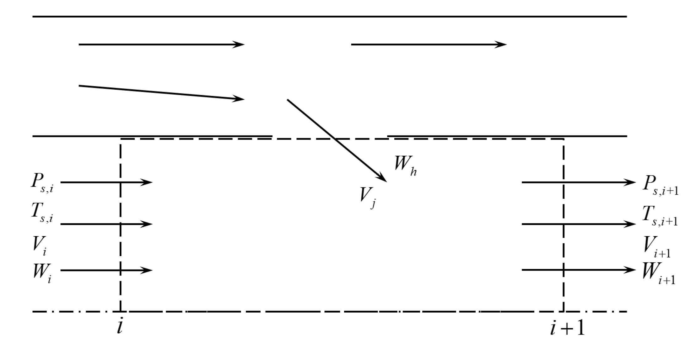
2.1. Calculation of Parameters along the Combustion Chamber

During the preliminary design of the annular combustion chamber, the thermodynamic parameters of the combustion chamber can be calculated after the preliminary determination of the combustion chamber structure. The 1D estimation of the combustor simplifies the complex flow in the combustor to the 1D constant flow and only considers the variation of flow parameters along the axial direction of the combustor, ignoring the non-uniformity in the radial direction. In the preliminary design of the combustion chamber, the basic assumptions for the calculation of aerodynamic and thermodynamic parameters along the combustion path are elucidated below [19,20]:
  • Assume 1D steady flow;
  • Ignore the internal friction and heat dissipation loss of the flame cylinder, but include the friction in the two channels (the channel between the flame cylinder and the casing) and the sudden expansion loss of the jet through the wall;
  • Assume the respective calculation section is in front of each row, and the effect of the flow rate of the row is not covered in the calculation of the aerodynamic and thermodynamic parameters of the i-th section;
  • Assume that the air entering the flame cylinder through the main combustion hole or the blending hole on section i completes the chemical reaction and mixing in the closed system composed of sections i to i + 1.
The flame cylinder consists of a main combustion zone, an intermediate zone, and a mixing zone. It is primarily capable of creating a stable place for combustion such that the fuel can be steadily and continuously burned in it, and it has the capability of organizing air distribution such that the temperature distribution at the outlet of the combustion chamber can meet certain requirements.
The calculation of the combustion process and the axial variation of the gas temperature in the flame cylinder is complex. Thus, approximate formulas are employed for calculation in engineering. The total gas temperature is determined based on the ideal constant total enthalpy before and after the gas reaction. Moreover, the temperature of the combustion products is calculated using a polynomial fitting method in the temperature range (400~1000 K) of the combustion chamber inlet, with the polynomial form expressed as follows:
T t , i = A 1 + A 2 α + A 3 α 2 + A 4 α 3
where Tt,i denotes the total temperature at section i; A1, A2, A3, A4 represent polynomial coefficients; and α expresses the residual air coefficient.
As depicted in Figure 1, the section from the leading edge of the i-th exhaust intake hole to the leading edge of the (i + 1)th exhaust intake hole is taken as the control body. For the selected control body, the average wall pressure is expressed as ( P s , i + P s , i + 1 ) / 2 . The momentum is conserved along the axial direction of the flame cylinder. The calculation formula of static pressure P s , i + 1 can be obtained by combining with the flow equation:
P s , i + 1 = I i + 1 + I i + 1 2 2 ( A i + A i + 1 ) W i + 1 2 R T s , i + 1 / A i + 1 A i + A i + 1
where Ps,i, Ii, Wi, Ai and R are the static pressure, momentum, inlet flow, flame cylinder area, and air constant at section i, respectively. The expression of Ii is as follows:
I i = P s , i A i + A i + 1 2 + W i V i
According to the flow equation, the velocity V i + 1 can be calculated as:
V i + 1 = W i + 1 R T s , i + 1 A i + 1 P s , i + 1
The velocity coefficient λ i + 1 is:
λ i + 1 = V i + 1 α c r , i + 1
where k is 1.4; and α c r , i + 1 is the local sound velocity, which can be determined by Equation (6):
α i + 1 = 2 k k + 1 R T t , i + 1
The static temperature T s , i is:
τ ( λ i + 1 ) = T s , i T t , i = 1 k 1 k + 1 λ i + 1 2
The total pressure P t , i is:
π ( λ i + 1 ) = P s , i P t , i = ( 1 k 1 k + 1 λ i + 1 2 ) k k 1

2.2. Combustion Chamber Performance Calculation Method

Based on the 1D calculation of the annular combustion chamber, the performance of the combustion chamber can be estimated, and whether the performance meets the requirements can be judged. This section mainly introduces the estimation of combustion efficiency, the total pressure recovery coefficient, the outlet temperature distribution factor (OTDF), and the NOx emission index.

2.2.1. Combustion Efficiency

In the combustion rate model, it is mainly assumed that the evaporation rate and the mixing rate are completed instantaneously. The main cause of combustion loss is the fuel not being sucked into the reflux area for combustion but directly into the mixing area. Using this model, Greenhough and Lefebvre [21,22] summed up the combustion efficiency ηB calculation formula of Equation (9):
η B = [ P t 3 A r e f ( P t 3 D r e f ) m exp ( T t 3 / b ) / W 3 ] [ Δ P L / q r e f ] 0.5 m
where qref, Dref, and Aref express the dynamic pressure head, flame cylinder diameter, and area at the reference section, respectively; ∆PL denotes the total pressure loss. In accordance with extensive combustion chamber experimental data, m = 0.75 and b = 300.

2.2.2. Total Pressure Recovery Coefficient

The total pressure recovery coefficient of the combustor represents the ratio of the total pressure at the combustor outlet to the total pressure at the inlet [23]:
σ B = P t 4 P t 3
where P t 3 and P t 4 denote the average total pressure of the inlet and outlet sections of the combustion chamber, respectively.

2.2.3. Outlet Temperature Distribution Factor

Since the high-temperature fluid at the outlet of the combustion chamber directly enters the first-stage guide blade of the turbine, if the temperature field is uneven, the thermal stress on the radial direction of the blade will be uneven, which will lead to the blade being damaged. Similarly, the uniformity of the temperature field at the outlet of the combustion chamber will greatly affect the safety and service life of the turbine working blade. It also has a certain influence on the pollutant discharge of the combustion chamber. Indicators to judge the uniformity of the temperature field at the outlet include the outlet temperature distribution factor (OTDF, also known as the maximum outlet unevenness), the radial temperature distribution factor (RTDF), and the circumferential temperature distribution factor (CTDF), etc. The OTDF is expressed as follows [24]:
OTDF = T t 4 max T t 4 T t 4 T t 3 = f ( L L D L × Δ P L q r e f )
where L L is the total length of the flame cylinder; D L is the diameter or height of the flame cylinder; and Δ P L / q r e f is the pressure loss coefficient of the flame cylinder.
For single-tube combustion chambers and circumferential combustion chambers, the OTDF is:
OTDF = 1 exp ( 0.070 L L D L Δ P L q r e f ) 1
For annular combustion chambers, the OTDF is:
OTDF = 1 exp ( 0.050 L L D L Δ P L q r e f ) 1
General requirement: OTDF∈[0.25, 0.35].

2.2.4. NOx Emission

In reference [25], Lefebvre pointed out that the generation of NOx in the combustion chamber was mainly determined by the following factors: the chemical reaction rate, the mixing rate, and the residence time. According to the above assumptions, for the diffusion flame mode of conventional combustors, the NOx prediction model was obtained by curve-fitting the emission data as:
E I NOx = 9 × 10 8 P 1.25 V c exp ( 0.01 T s t ) / m ˙ a / T p z
where E I NOx is the NOx emission index; P is the inlet pressure; Vc is the flame volume; T s t is the chemically appropriate flame temperature; m ˙ a is the combustion chamber air flow; and Tpc is the primary combustion zone temperature.

3. Preliminaries

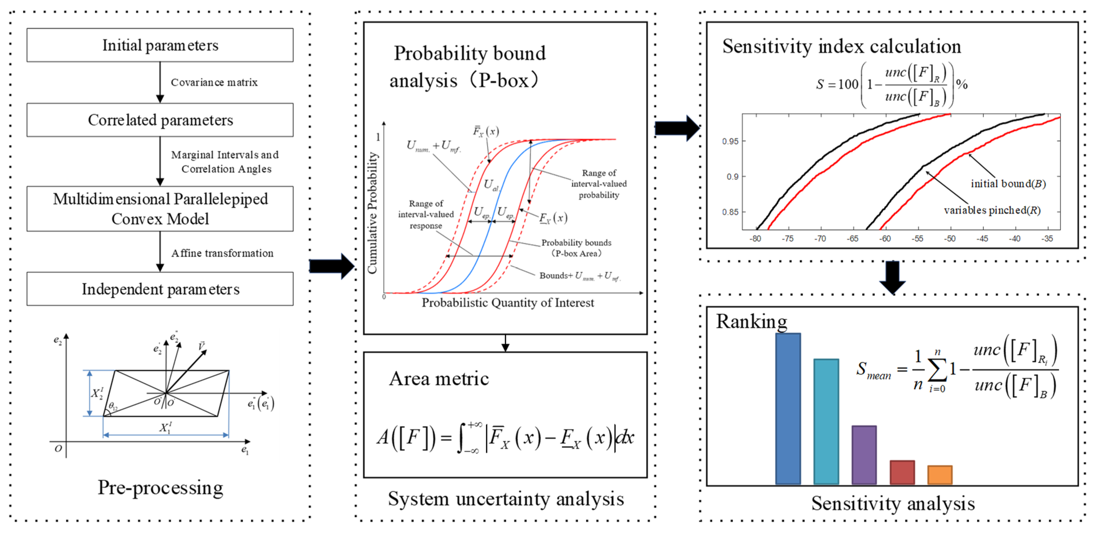
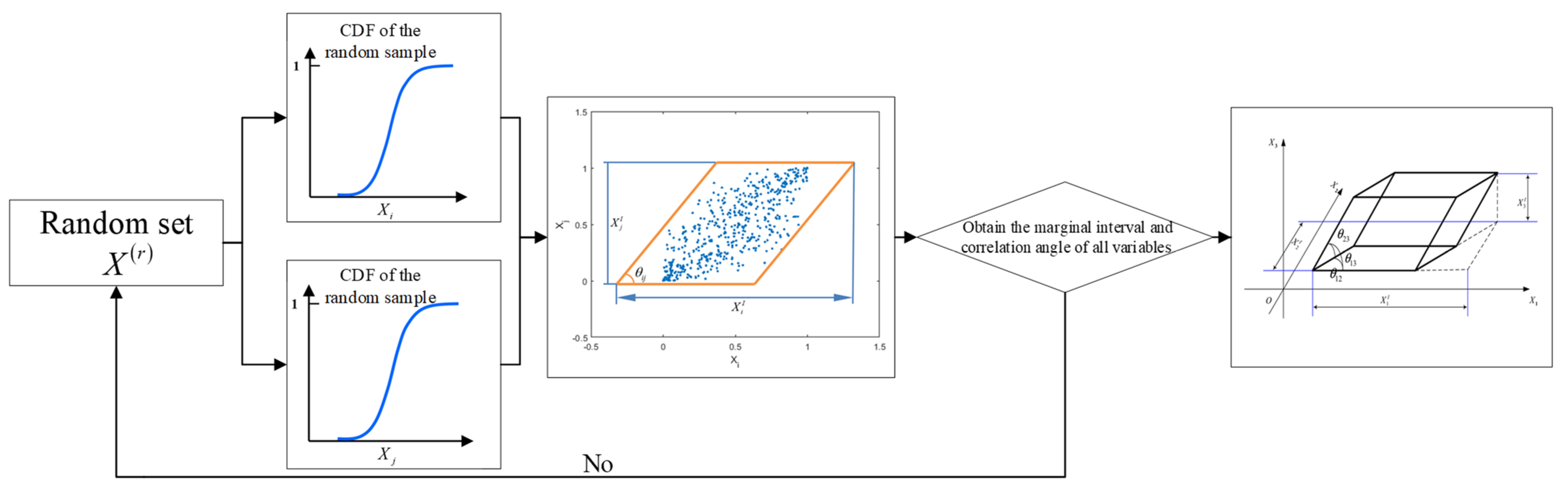
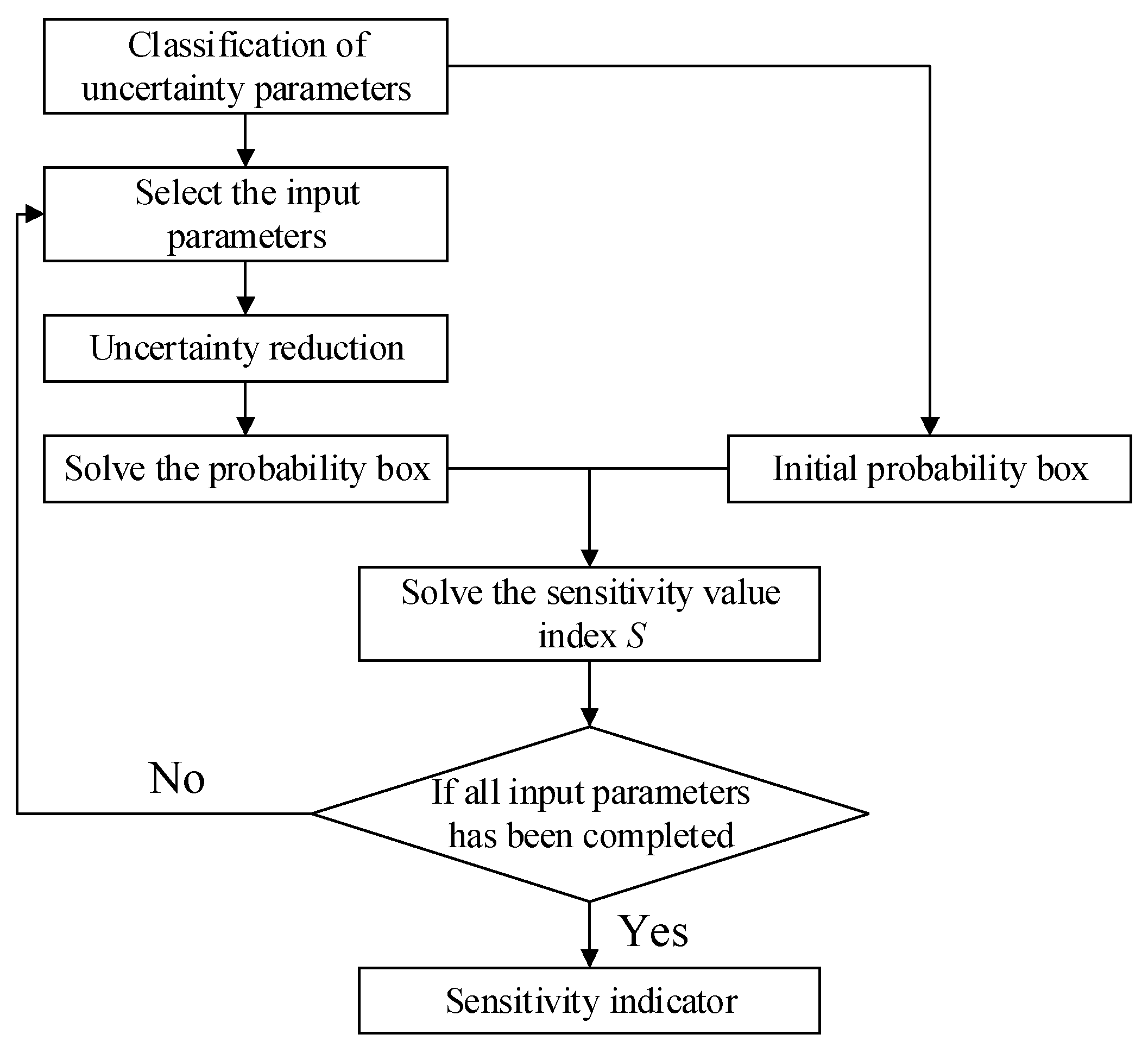
3.1. Analysis Process

In this section, the entire workflow of system uncertainty analysis [26] is presented, which comprises the following three steps (Figure 2).
i.
Preprocessing: This step aims to construct the relevant variables first and then construct the uncertainty domain to represent the relevant features. Moreover, an affine coordinate system is introduced to transform the correlated variables into independent variables to lay a solid foundation for sensitivity analysis.
ii.
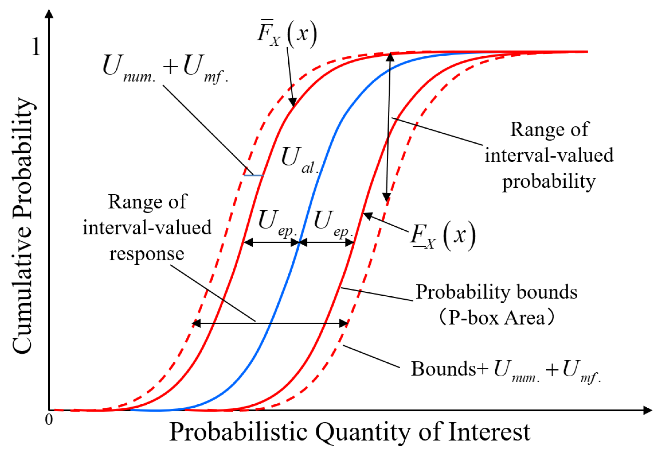
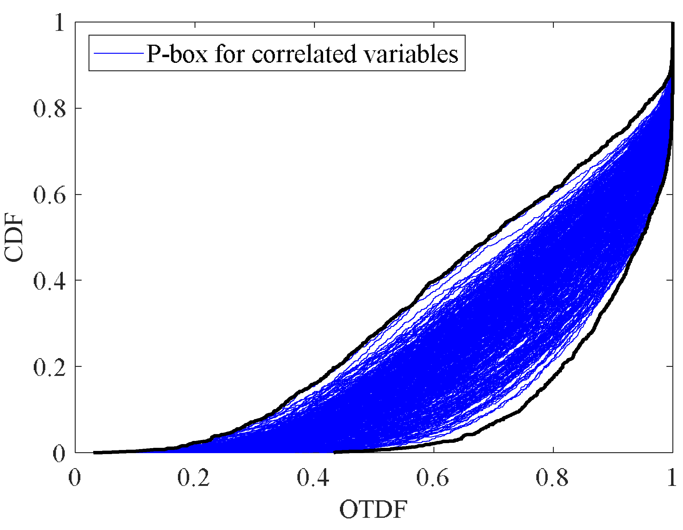
System uncertainty analysis: The input and output of the system are quantified using a p-box. The relevant and independent situations are analyzed and then compared. The area of the region between the upper and lower boundaries of the p-box is defined as the uncertainty metric.
iii.
Imprecise sensitivity analysis: The sensitivity calculation is biased due to the effect of epistemic uncertainty. The average value of the sensitivity index serves as the criterion to measure the final sensitivity analysis so as to reduce the effect of bias.

3.2. Pre-Processing

The multi-dimensional parallelepiped model is capable of considering independent and correlated uncertain variables under a unified framework simultaneously while addressing the multi-source uncertainty problem with the coexistence of two types of variables. The uncertainty domain Ω can be constructed only by knowing the variation range of the parameters, i.e., the interval and the correlation between any two parameters. Geometrically, the constructed uncertainty domain is a multi-dimensional parallelepiped and convex set. The following is an example of constructing a convex model in a multi-dimensional space [13]:
In the three-dimensional space, by sampling the parameters, the uncertainty domain Ω constructed is a parallelepiped (Figure 3). One side of the parallelepiped is set parallel to the XY coordinate plane. The marginal intervals X 1 I , X 2 I and X 3 I represent the uncertainty ranges of the variables, respectively, and θ12, θ13, and θ23 represent the correlation angles of any two variables among the three variables.
For the n-dimensional space, the uncertainty domain Ω is a multi-dimensional parallelepiped. X i I ( i = 1 , 2 , ... , n ) represents the marginal interval of the variable, and the correlation degree between the two variables X i and X j is expressed by the correlation angle between the variables. Furthermore, for the convenience of description, the correlation coefficient ρ i j between variables is defined as:
ρ i j = X j W X i W tan θ i j , θ i j [ arctan X j W X i W , π arctan X j W X i W ] , ρ i j [ 1 , 1 ]
When θ i j = arctan X j W X i W , ρ i j = 1 , and X i and X j have a linear positive correlation (Figure 4a). When θ i j = 90 ° , ρ i j = 0 , X i and X j are independent, and the parallelogram model degenerates into an interval model (Figure 4b). When θ i j = π arctan X j W X i W , ρ i j = 1 , and X i and X j are linearly negatively correlated (Figure 4c).
In brief, when the correlation coefficients of all variables are 0, the multi-dimensional parallelepiped model degenerates into an interval model, i.e., the interval model is actually a special case of the parallelepiped.

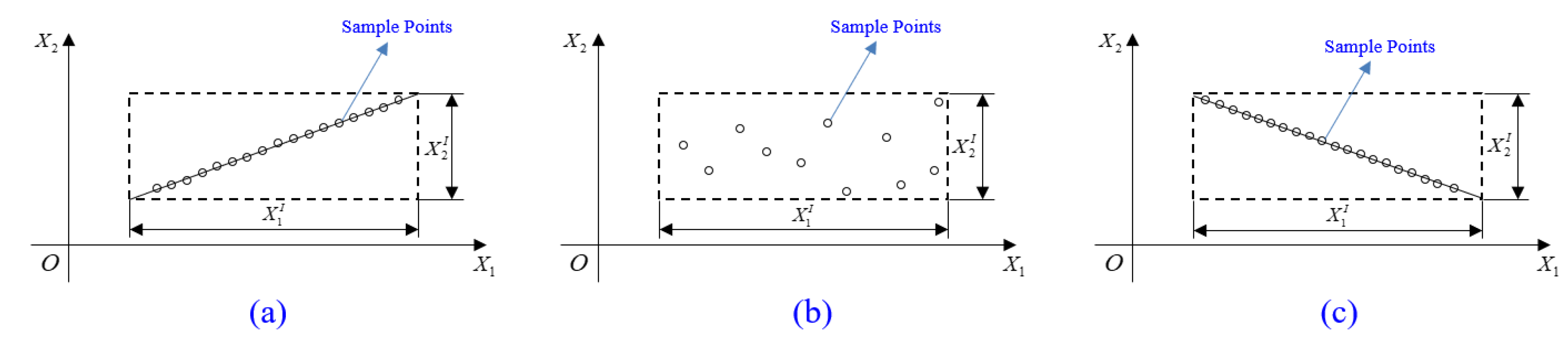
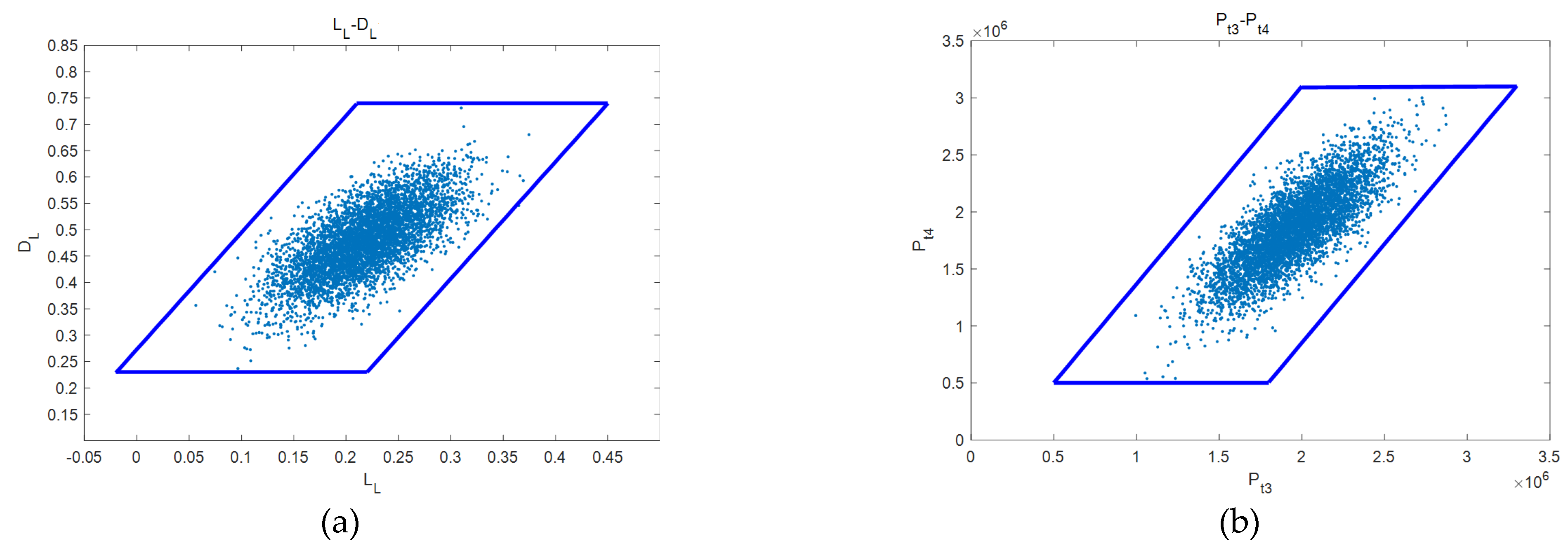
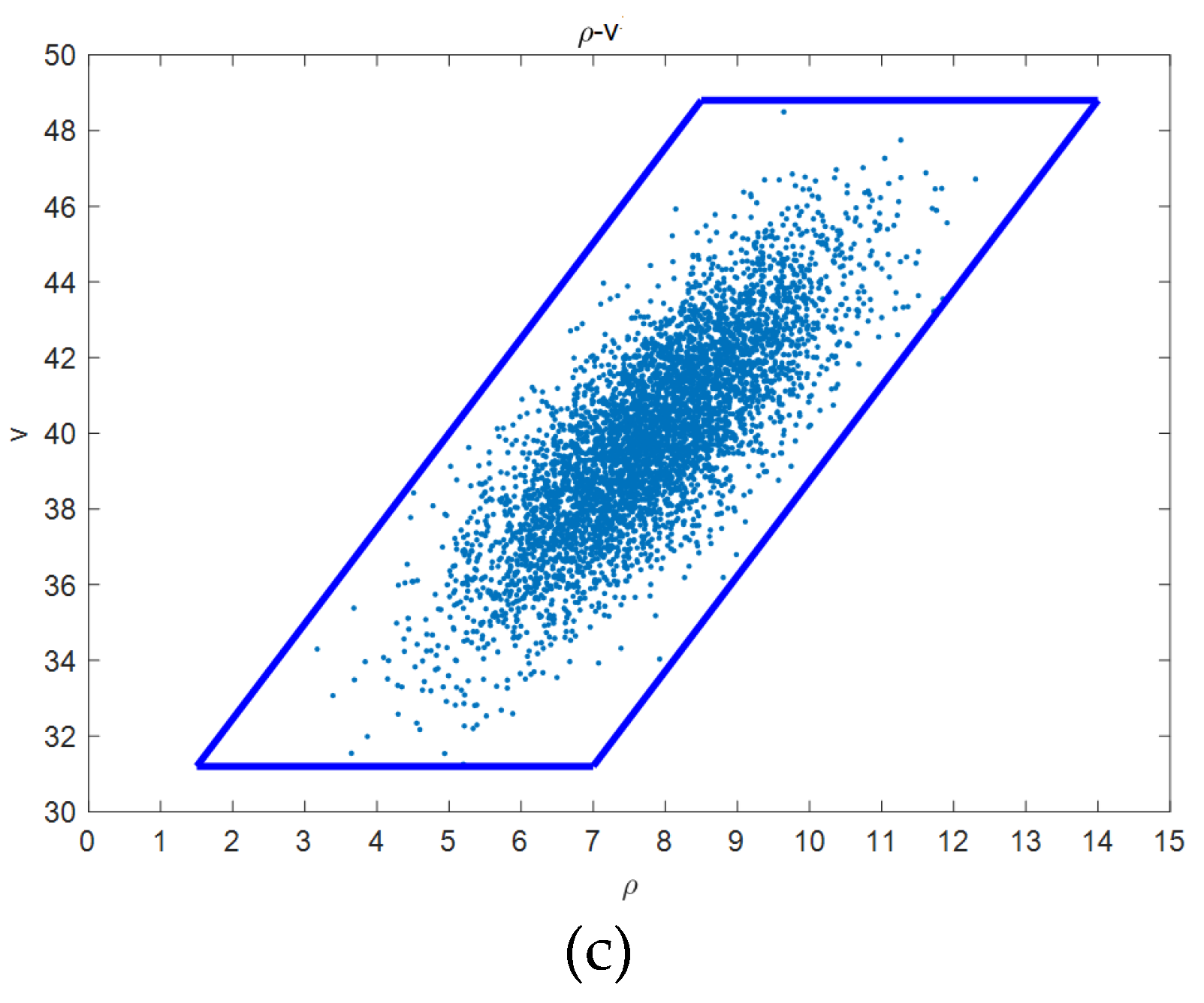
3.3. Uncertainty Domain

The construction of the uncertainty domain requires the marginal interval of all uncertainty parameters and the correlation of any two uncertainty parameters. Next, a method is presented to build a multi-dimensional parallelepiped model based on simulation samples (Figure 5). The specific steps are elucidated as follows [27]:
Step 1: Take any two uncertain variables Xi and Xj, ij.
Step 2: Extract the sample values of Xi and Xj from the sample set X(r) to obtain a two-dimensional (2D) sample set ( X i ( r ) , X j ( r ) ), r = 1, 2, …, m.
Step 3: In the XiXj 2D variable space, construct a parallelogram containing all samples ( X i ( r ) , X j ( r ) ), r = 1, 2, …, m, to obtain the marginal of the variable Intervals X i I and X j I , the correlation angle θij, and the correlation coefficient ρij.
Step 4: Repeat the above steps for any two uncertain variables, and obtain the marginal interval and correlation coefficient of all uncertain variables.
Step 5: Establish a multi-dimensional parallelepiped convex model in accordance with the obtained marginal interval and the correlation coefficient of the respective variable. The established multi-dimensional parallelepiped model should satisfy the following criteria: (1) The variation range along the respective axis is equal to the corresponding marginal interval; and (2) The angle of each two sides of the parallelepiped model is equal to the corresponding correlation angle.

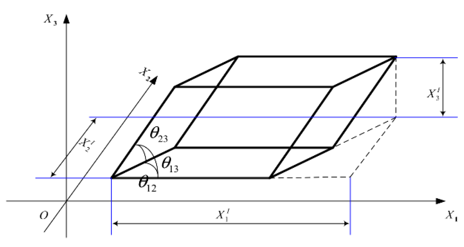
3.4. Affine Transformation

In the above analysis, a multi-dimensional parallelepiped model can be constructed through the sample points to describe the uncertainty of the parameters. However, it is difficult to use the uncertainty domain formed by the multi-dimensional parallelepiped to characterize the uncertainty analysis with an explicit function. This section will introduce a new coordinate system, the affine coordinate system, which provides an effective solution to the problem. In the affine coordinate system, the angle between the axes is no longer constant (equal to 90°), but equal to the correlation angle between the corresponding variables [13,27]. Through affine transformation, the parallelogram model in the initial parameter space can be transformed into an interval model in the affine space, which provides great help for the subsequent uncertainty analysis.
In the n-dimensional parallelepiped model, the initial space rectangular coordinate system is recorded as { O ; e 1 , e 2 , , e n } . The relevant angle is converted into the angle θij between the axes of the affine coordinate system. The corresponding affine coordinate system is established as { O ; e 1 , e 2 , , e n } . The affine coordinate system and the cartesian coordinate system have the following relation:
{ e 1 = a 11 e 1 + a 12 e 2 + + a 1 n e n e 2 = a 21 e 1 + a 22 e 2 + + a 2 n e n e n = a n 1 e 1 + a n 2 e 2 + + a n n e n
The matrix form is:
( e 1 e 2 e n ) T = A T ( e 1 e 2 e n ) T
where the matrix AT is an affine coordinate transformation matrix, and aij are the weight coefficients, representing the elements of the matrix AT, which can be obtained according to Equation (18):
a i j = { 0 , j > i cos θ k m = 1 j 1 a i m a j m a j j , j < i 1 l = 1 j 1 a i l 2 , j = i
In Equation (18), θ k is related to θ i j by k = ( 2 n j ) ( j 1 ) 2 + ( i j ) .
Combined with coordinate transformation, the mapping relationship between the initial parameter space and the final affine space for n-dimensional problems is expressed as:
( x 1 x 2 x n ) T = A ( x 1 x 2 x n ) T + ( x 1 L + x 1 U 2 x 2 L + x 2 U 2 x n L + x n U 2 ) T
The correlation between the parameter interval radii before and after affine transformation is written as:
( x 1 W x 2 W x n W ) T = A 1 ( x 1 W x 2 W x n W ) T

4. Probability Bound Analysis

4.1. Source of Uncertainty

Theoretically, the sources of uncertainty in simulation models fall into three main categories, i.e., the model form uncertainty, the numerical uncertainty, and the input uncertainty, as summarized by Oberkampf [28]. Model form uncertainty arises from the process of abstraction and formulation of mathematical models to approximate physical systems through simulation models. This type of uncertainty is usually estimated by model validation [29]. Numerical uncertainties are inherent in simulations since most simulation models comprise a set of nonlinear differential equations, whereas numerical solution methods are required in the model output calculation, thus causing numerical uncertainties (e.g., time and space discretization errors in the continuous model formulation, insufficient iterative convergence of the numerical solution, as well as rounding errors in the computational system) [30]. In verification and validation, convergence and rounding errors are considered negligible in the simulation platform, whereas discrete errors can be evaluated using the grid convergence method mentioned by Roache [31]. Input uncertainty covers uncertainty in all data required to fully specify the model or the model’s intrinsic parameters and modeling constants as well as the model inputs defined by the evaluation model. The model inputs can fall into initial conditions, boundary conditions, and geometric representation. In most cases, the above-described data cannot be determined accurately due to insufficient experimental data or errors in measurements.
The different natures of uncertainty (i.e., aleatory uncertainty and epistemic uncertainty) should be distinguished once all sources of uncertainty are identified, especially in the case of input uncertainty. Aleatory uncertainty is also known as chance uncertainty, where the specific value of a random variable cannot be accurately predicted, but the population of that variable follows a specific probability distribution that can be inferred from the population. Thus, aleatory uncertainty can be modeled and characterized by classical probability theory, and this type of uncertainty is generally fixed and incommensurable. Epistemic uncertainty caused by imperfect knowledge can usually be reduced by empirical effort, and epistemic parameters are constant and unknown but not naturally varying. Interval forms provide a more natural way to model imperfect knowledge or epistemic uncertainty but are not suitable for characterizing aleatory uncertainty. Since intervals can characterize epistemic uncertainty, and probabilities can characterize aleatory uncertainty, the combination of the two has led to the development of imprecise probability theory. Imprecise probability theory refers to an uncertainty theory where the modeling process should consider variability and imprecision, and the unknown and the uncertainty should be strictly distinguished. Imprecise probability theory comprises probability bounds analysis, Dempster–Shafer evidence theory [32,33], random set theory [34], fuzzy set theory [35], polymorphic uncertainty theory [36], and information-gap theory [37]. To be specific, probability bound analysis (PBA) [38,39] can be explored based on a defined probability box (p-box).

4.2. Probability Box

Probabilistic bound analysis is based on a strict distinction between aleatory and epistemic uncertainty. In the presence of hybrid uncertainty, double-layer Monte Carlo sampling combines the interaction of aleatory uncertainty and epistemic uncertainty so that the Quantities of Interest (QoI) produces a cumulative distribution function (CDF) of gathering. Such ensembles are broadly interpreted as probabilistic bounds on QoI and inferred metrics from the resulting p-box. Accordingly, the p-box indicates that, under a given uncertainty condition, QoI cannot be expressed as an exact probability but as an interval-valued probability. Using the p-box to represent uncertainty in QoI caused by input uncertainty is also beneficial to clearly describe the total output uncertainty of QoI in PBA. Model formal uncertainty and numerical uncertainty, which are often interpreted as epistemic uncertainty, are added to the probability bounds of the p-box [40], as shown in Figure 6.
In Figure 6, the blue line denotes the CDF of QoI obtained by transferring uncertainty through the model with only random uncertainty. Based on a single CDF, the epistemic uncertainty is gradually included to obtain a set of CDFs, and the red line represents probability bounds from the CDFs. Moreover, model formal uncertainty and numerical uncertainty are introduced to the probability bounds, such that the p-box is expanded. The generated p-box diagram indicates that a given probability or response level can derive the corresponding interval-valued response range or interval-valued probability range, respectively [41].
The specific mathematical expression of the p-box is F X I = { F ( x ) : x , F _ X ( x ) F X ( x ) F ¯ X ( x ) } , where F X I denotes the probability distribution function space in the real domain ℜ, F _ X ( x ) , F X ( x ) , F ¯ X ( x ) : [ 0 , 1 ] . F ¯ X ( x ) = 1 P _ ( X > x ) and F _ X ( x ) = P _ ( X x ) are the upper and lower probability boundaries of the p-box, respectively, and the region enclosed by the upper and lower boundaries can be expressed by the area A ( [ F ] ) according to Equation (21).
A ( [ F ] ) = + | F ¯ X ( x ) F _ X ( x ) | d x

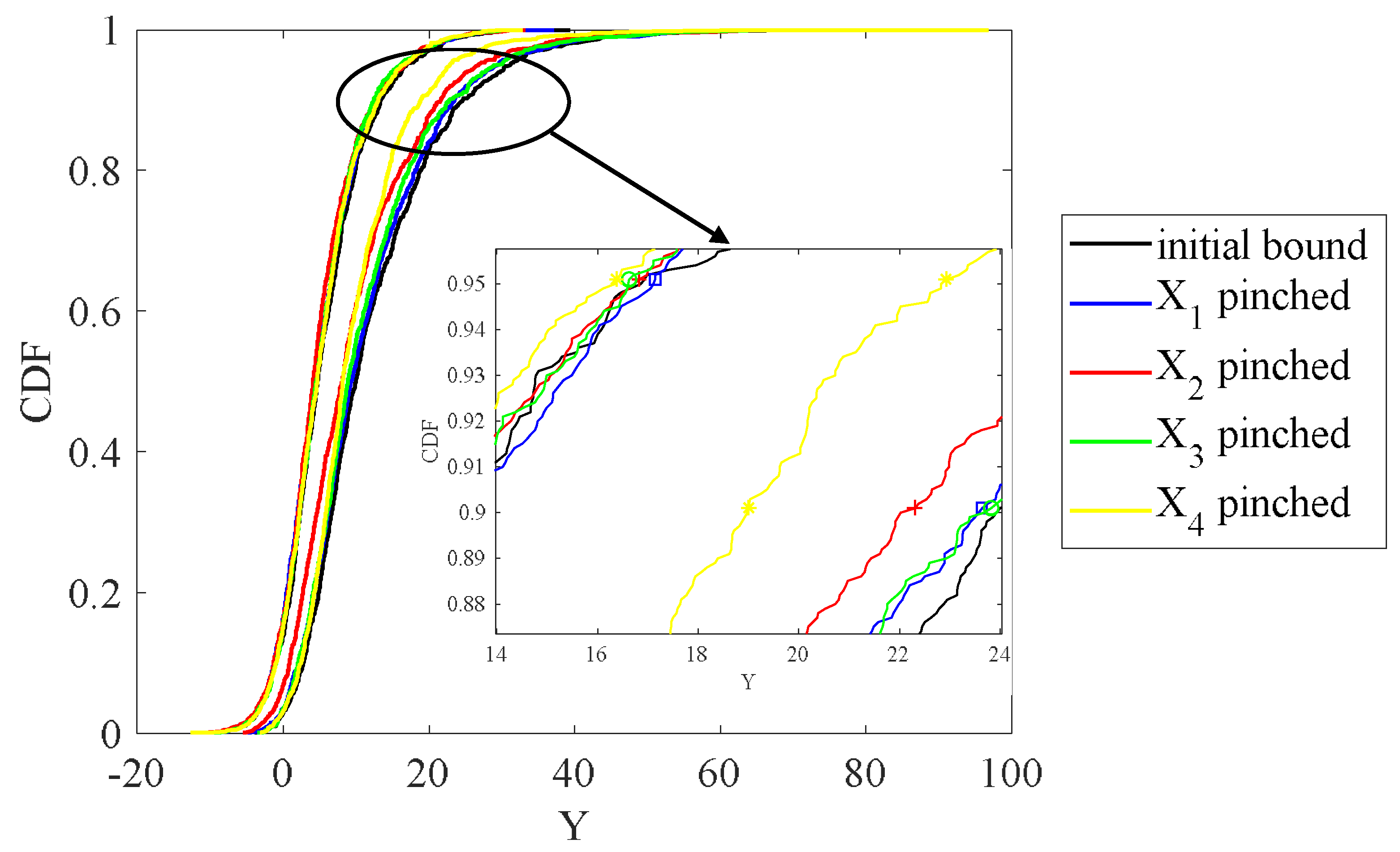
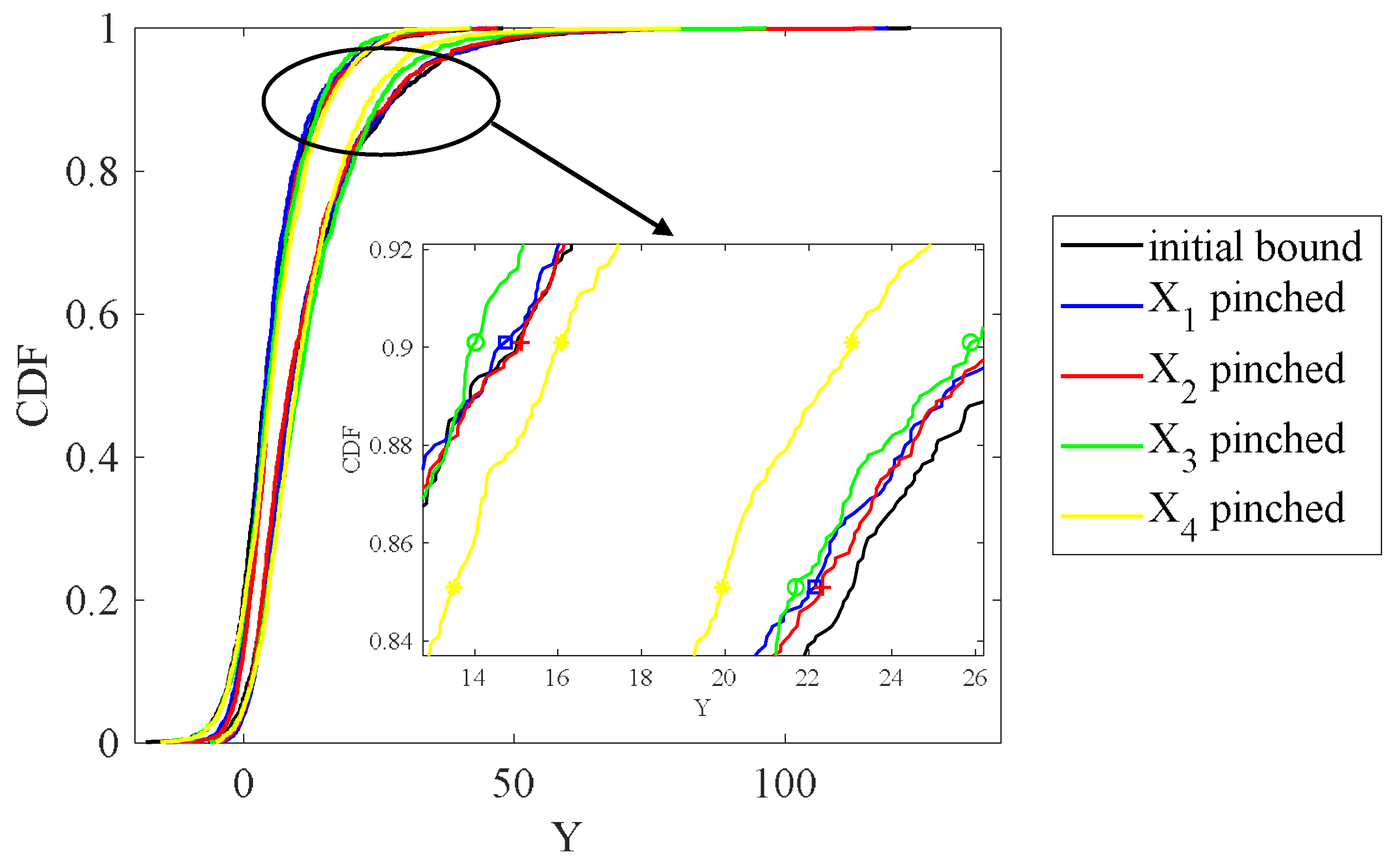
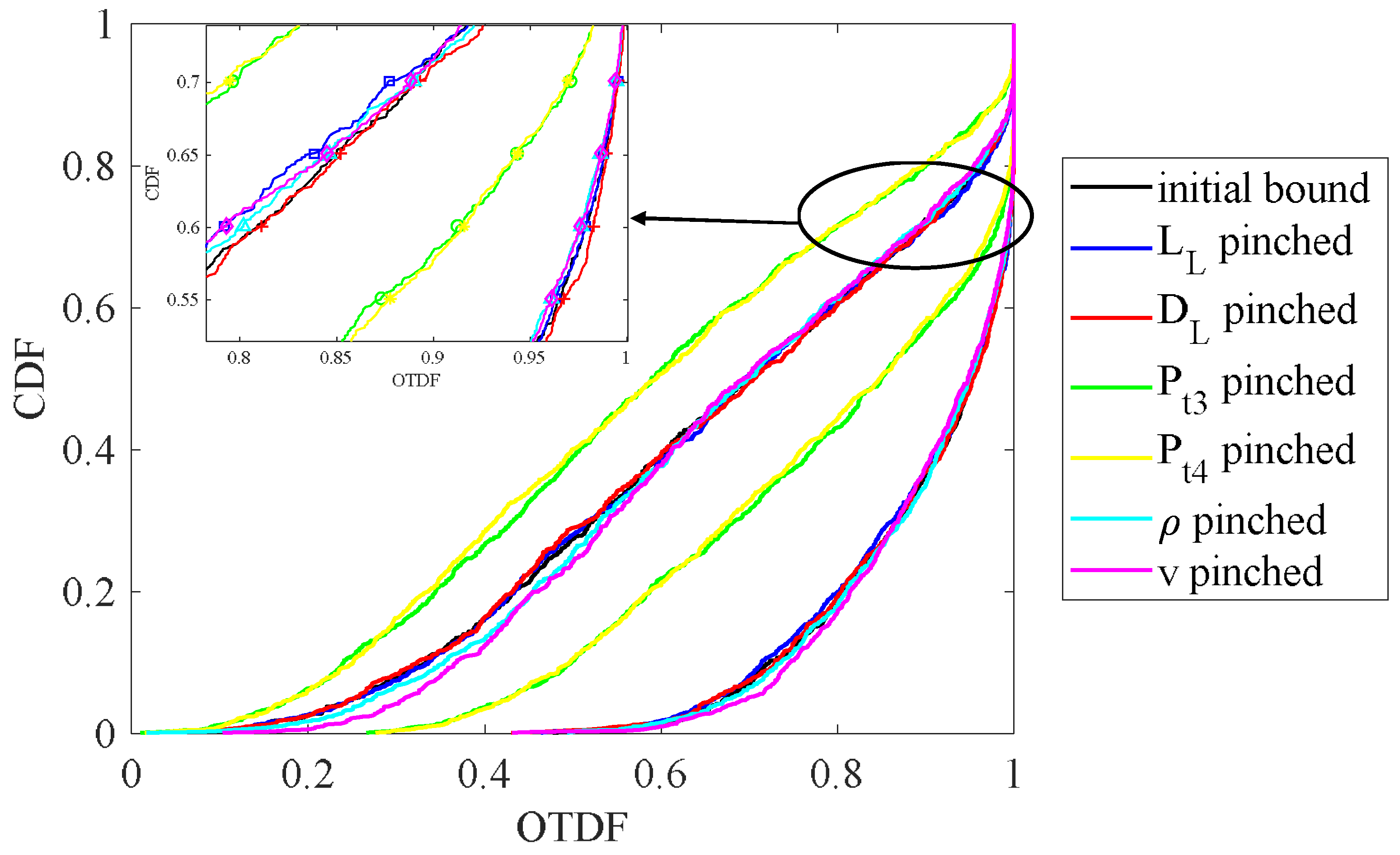
4.3. Sensitivity Analysis

Sensitivity analysis is to study the effect of system input uncertainty on the output response. There are two basic reasons for system sensitivity analysis: one is to understand how the conclusions and inferences obtained from the evaluation depend on its input conditions; the other is to improve the input conditions. Estimate and then maximize the reliability of the system [42]. Given the significance of sensitivity analysis in interpreting calculated results, many analytical disciplines attach great importance to this approach. However, in practical engineering applications, because the precise distribution is unknown, interval values are generally used for uncertainty prediction, and the conventional sensitivity analysis method fails due to the imprecise form of input variables [43]. Ferson [44] proposes a p-box to characterize this type of uncertainty by using a pinching method to evaluate the hypothetical impact of additional empirical knowledge on output uncertainty.
Using sensitivity analysis methods to identify the input variables that have the greatest impact on the output requires estimating the value of additional empirical information [45]. For this purpose, one approach is to evaluate the degree to which the uncertainty of the calculation is reduced with additional knowledge about the input. This can be done by comparing the uncertainty before and after reducing the input variable, i.e., by substituting a value without uncertainty, which is usually speculative. Reducing a variable means reducing its uncertainty, and quantifying this effect allows an evaluation of the input’s contribution to the total uncertainty of the calculation [46]. The estimate of the variable information value depends on the uncertainty present in that variable and how it affects the uncertainty in the final output response [47]. The sensitivity can be calculated by the following expression:
S = 100 ( 1 u n c ( [ F ] T ) u n c ( [ F ] B ) ) %
where B represents the original benchmark input parameter; T represents the input parameter after reducing uncertainty; and unc() represents the measure of output uncertainty.
The calculated sensitivity S is an estimate of the value of additional empirical information for the input variable, and when the input variable is replaced by the estimated value, the sensitivity S will reflect the reduction in the percentage of uncertainty for that variable. Uncertainty reduction is performed on the respective input variable in turn, and the input variables are sorted according to the calculation of the sensitivity S. Unlike the global sensitivity analysis of the Sobol index based on variance decomposition, the sum of the sensitivity S obtained by the uncertainty reduction of all input variables in the above method usually does not reach 100%. In principle, multiple input variables can also be reduced simultaneously to study the effects of their interactions.
The unc() parameter is similar to the variance which is used to calculate the sensitivity index in the global sensitivity analysis based on variance decomposition. In the probability boundary analysis, the p-box is the envelope of all possible CDFs of the parameters, and the area between the upper and lower limits of the output p-box can serve as the uncertainty measure, i.e., the area of the p-box can serve as the output uncertainty unc(). Figure 7 illustrates the process of measuring and calculating the sensitivity index. When the p-box approaches an exact probability distribution, all epistemic uncertainties have been eliminated, only aleatory uncertainties exist, and the area approaches zero. If the uncertainty measure is a scalar, the sensitivity will also serve as a scalar and can be sorted [48,49].
There are many ways to reduce the uncertainty of input parameters. Using different methods to reduce uncertainty will result in different sensitivity indexes, such that great differences will be generated in the estimation of the overall value of information. However, the sensitivity ranking of the respective input variable will not be affected. There are usually three ways, as follows [26]:
(i)
Use a specific probability distribution to replace the uncertainty input parameters; the specific probability distribution method only eliminates the epistemic uncertainty of the parameter, and does not affect its aleatory uncertainty;
(ii)
Use the fixed value to replace the uncertainty input parameter; the fixed value method eliminates the aleatory uncertainty and epistemic uncertainty of the parameter at the same time;
(iii)
Use the zero-variance interval method to replace the uncertainty input parameter; the zero-variance interval method only eliminates the aleatory uncertainty, and preserves the effects of epistemic uncertainty.
Considering that aleatory uncertainty is difficult to eliminate, this study chooses method (i) to reduce uncertainty, eliminate epistemic uncertainty, and only represent aleatory uncertainty. Since the value of the input parameter is unknown during reduction, different parameter values are used in the sensitivity analysis to cause a change in the sensitivity index, which is called bias. In order to reduce the effect of bias, a new sensitivity index is proposed based on Equation (22), which adopts the average value of all sensitivity index values, as shown in Equation (23):
S m e a n = 1 n i = 0 n 1 A ( [ F ] R i ) A ( [ F ] B )
where n is the number of times to perform uncertainty reduction.

5. Applications

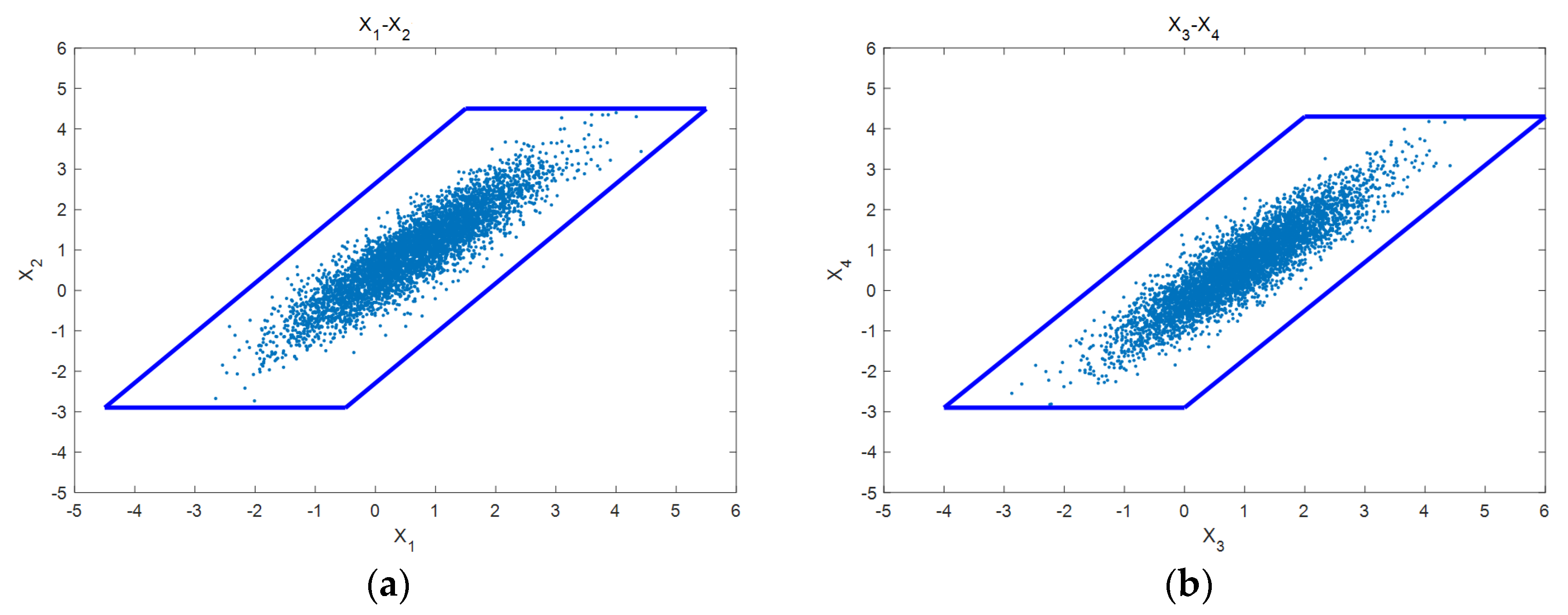
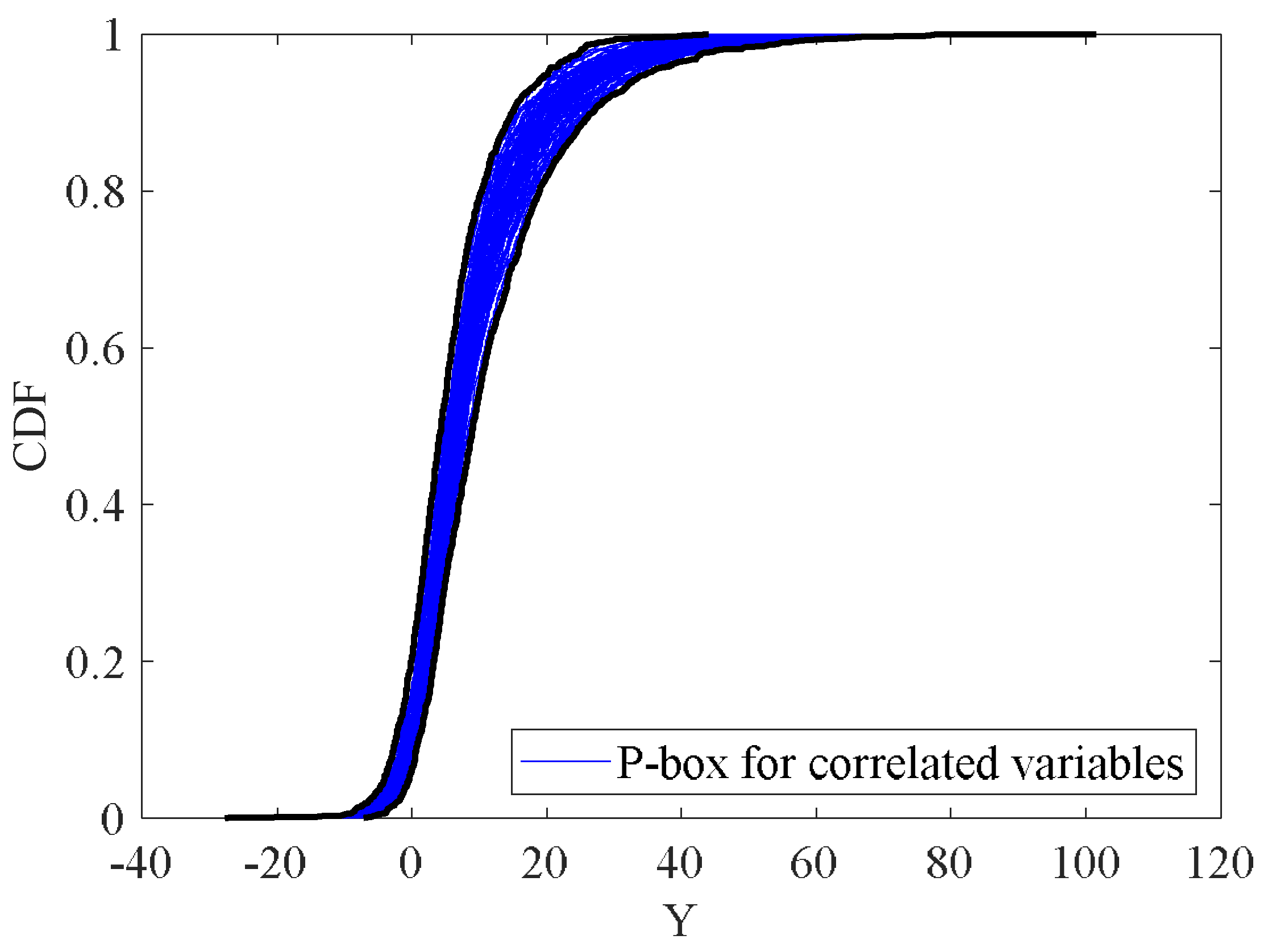
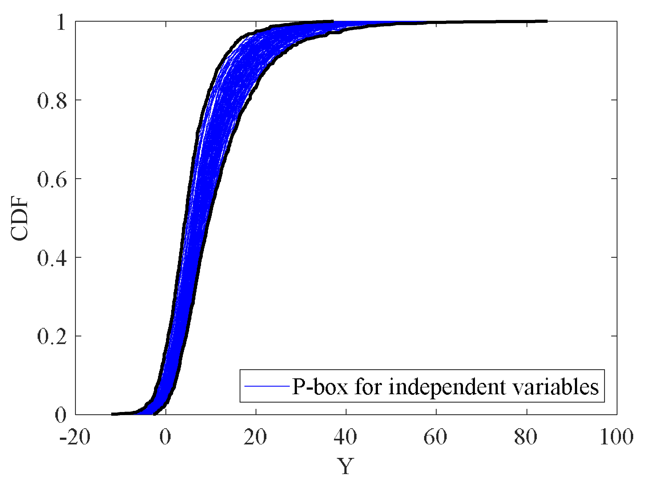
5.1. Four-Dimensional Function

5.1.1. Problem Statement

Consider the following analytical function [50]:
Y = G ( X ) = X 1 + 3 X 2 + X 3 2 + 3 X 4 2 + X 1 X 3 + X 2 X 4
Four of the input variables Xi (i = 1, 2, 3, 4) are random variables subjected to standard normal distribution. Given the effect of epistemic uncertainty, the mean of the input variables is set as μ X i I = [ 0.2 , 1 ] , and the variance is set as σ x = 1 . The correlation angle between variables X1 and X2 is set as θ21 = 26° (correlation coefficient ρ = 0.9), the correlation angle between variables X3 and X4 is set as θ43 = 26° (correlation coefficient ρ = 0.9), and the variables both show a strong correlation. Table 1 lists the distribution of the variables.

5.1.2. Uncertainty Domain

The correlations between the above analytic function variables are analyzed and expressed with uncertainty domains. First, a parallelogram approximated by the sample is generated in the 2D parameter spaces X1X2 and X3X4 (Figure 8a,b). The correlation between the variables X1 and X2, as well as X3 and X4, is well presented by the parallelogram. Under the uncertainty domain, the preparations are made for the subsequent establishment of an affine coordinate system and the conversion of dependent variables into independent variables for sensitivity analysis.

5.1.3. Sensitivity Analysis

Two cases of variable correlation as well as variable independence are considered separately. Since the input parameters of function Y contain a mixture of aleatory and epistemic uncertainties, p-box uncertainty analysis is performed on function Y to study the problems of uncertainty propagation and quantization, determine the p-box global sensitivity of the uncertain input parameters to the output response, and then filter out the important and minor variables.
The uncertainty of the input parameters Xi (i = 1, 2, 3, 4) is propagated through the function G(X) to obtain the probability box Y. When reducing the epistemic uncertainty parameter in it, the probability boundary corresponding to Y will also be changes happened.
First, p-box uncertainty analysis is performed for the variables Xi (i = 1, 2, 3, 4) with correlation, and 1000 CDFs of Y are taken to obtain the p-box of Y under the initial conditions, as shown in Figure 9. The uncertainties of the input parameters X1~X4 are reduced using the pinching method, the epistemic uncertainty is eliminated, and the aleatory uncertainty is retained using a specific probability distribution to calculate the p-box after the corresponding reduction of uncertainty (Figure 10). Compared with the initial boundaries, the boundaries of the respective input variables are reduced to different degrees, while the curves in Figure 10 may have crossed and overlapping parts, and it is not possible to directly compare the uncertainty parameter space of the p-box. Thus, defining a metric to quantify the system uncertainty parameter space is beneficial to further quantify the sensitivity. From the method of area metric mentioned in Section 4.2, the area between the upper and lower boundaries of the p-box serves as the area to perform the uncertainty metric and thus the sensitivity analysis for the respective input parameter.
The different values of the means can cause a certain bias in the sensitivity since a specific probability distribution is selected for uncertainty reduction. According to Section 4.3, it is proposed to use Equation (23) to calculate the mean value of the sensitivity index to reduce the effect of its bias, and the calculation results are listed in Table 2. As depicted in Table 2, the mean values of the sensitivity indicators for the four parameters are well distinguished, where X4 and X1 are the most sensitive and the least sensitive, respectively.
Considering the existing correlated variables, an affine coordinate system is introduced into the uncertainty domain. The affine coordinate transformation matrix A can be obtained by the correlation angle between the parameters:
A = ( 1 0 0 0 0.9000 0.4359 0 0 0 0 1 0 0 0 0.9000 0.4359 )
B is set as ( A T ) 1 , and the correlation between the parameters in the initial space and the affine space is obtained by Equation (26) as:
( X 1 X 2 X 3 X 4 ) = ( 1 2.0647 0 0 0 2.2941 0 0 0 0 1 2.0647 0 0 0 2.2941 ) ( V 1 V 2 V 3 V 4 )
The original problem can then be equated to a hybrid aleatory and epistemic uncertainty problem with mutually independent variables, and a p-box sensitivity analysis is conducted on the transformed independent variables using the pinching method. As depicted in Figure 11, based on the hybrid aleatory and epistemic uncertainty characterized by the p-box, forward uncertainty propagation is performed to obtain the p-box corresponding to the response Y. The uncertainty reduction is performed sequentially for the input parameters X1~X4 to determine the corresponding reduced p-boxes (Figure 12). Likewise, the improved Equation (23) is used to calculate the sensitivity index values S for the respective input parameter, and the results are listed in Table 2. As depicted in the table, the sensitivity indexes obtained in the case of considering correlation are not consistent with those in the case of not considering correlation, indicating that the correlation between variables sometimes affects the sensitivity analysis, which may cause greater uncertainty analysis errors if the correlated variables are assumed as independent variables for analysis.

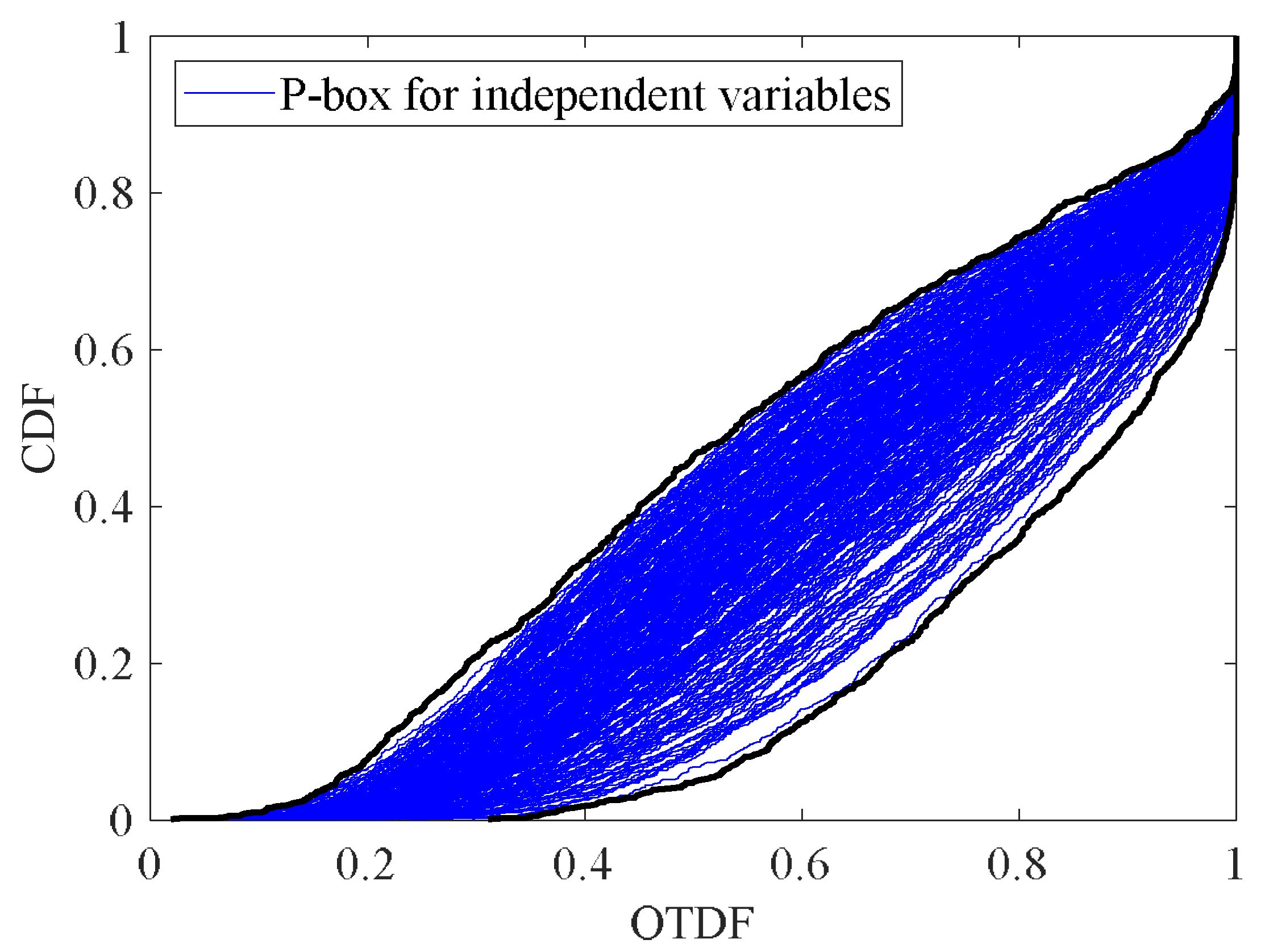
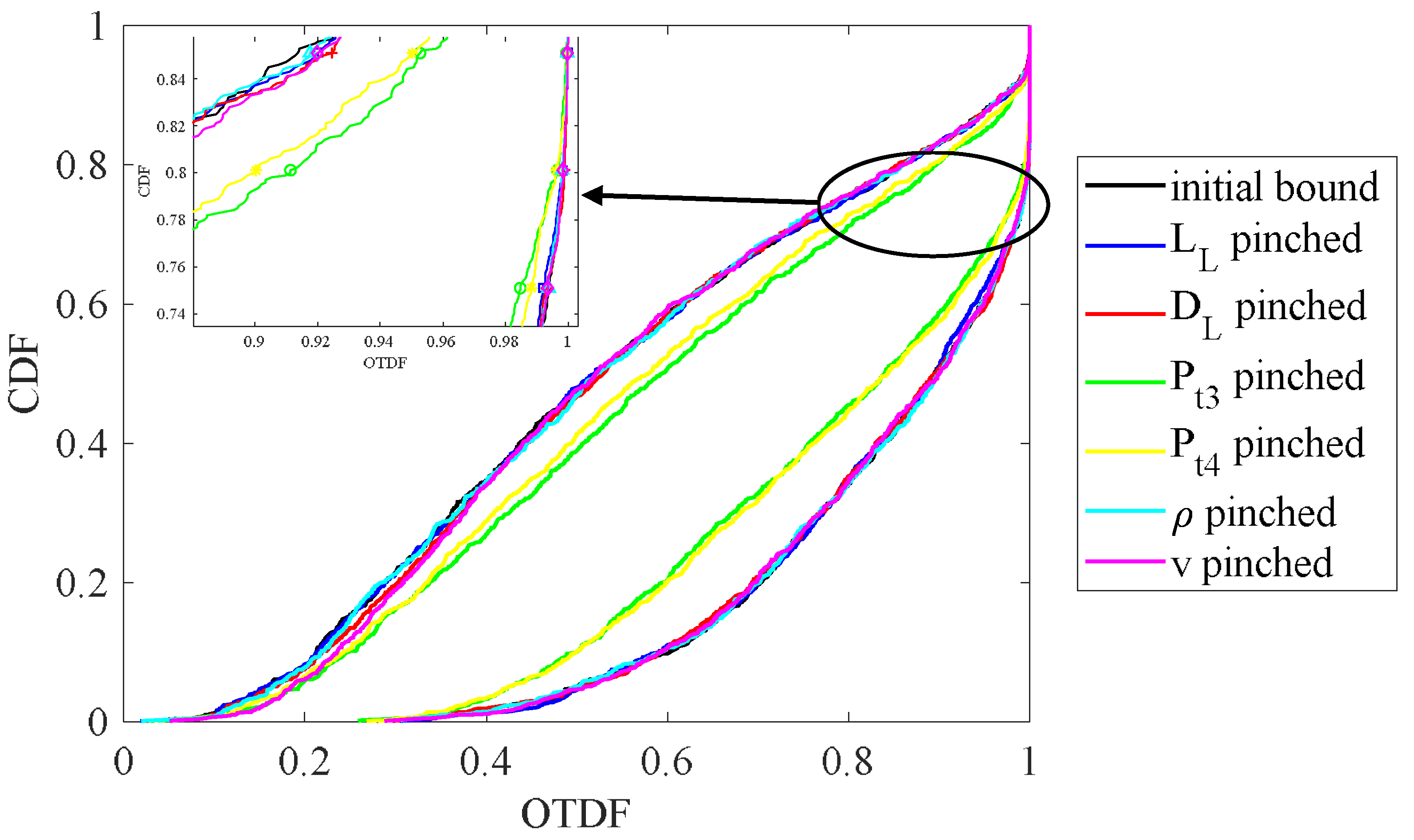
5.2. The Outlet Temperature Distribution Factor

The aero-engine has become the most widely used gas turbine engine. The combustion chamber is one of the core components of the aero-engine to achieve energy conversion. Its performance parameter (OTDF) indicates the ratio between the maximum temperature exceeding the average at the outlet of the combustion chamber and the temperature rise of the combustion chamber, which has a significant effect on the safety and service life of turbine blades. In this section, imprecise p-box sensitivity analysis based on the multi-dimensional parallelepiped model is conducted to analyze the effect of uncertain input parameters on OTDF. According to Equation (13), where the flame cylinder length is LL, the flame cylinder diameter is DL, the inlet pressure is Pt3, the outlet pressure is Pt4, the flame cylinder inlet density is ρ, and the reference flow rate is v. These parameters are the hybrid uncertainty parameters, and the serial numbers of the five parameters are recorded as 1, 2, 3, 4, 5, and 6 in order. Table 3 lists the distribution features of parameters.
Assuming that there are correlations between LL and DL, Pt3 and Pt4, and ρ and v with correlation coefficients of 0.7, 0.8, and 0.8, respectively, and that the correlation angles between the parameters obtained from the samples are 46°, 37° and 37°, respectively, the uncertainty domain is constructed using a multi-dimensional parallelepiped model, as shown in Figure 13.
First, the p-box uncertainty analysis of OTDF is conducted by considering the case of correlation between variables. As depicted in Figure 14, the 1000 CDFs of OTDF are taken to form the p-box under the initial conditions. As depicted in Figure 15, using the pinching method to reduce the uncertainty of the respective input parameters 1~6, a specific probability distribution is selected to eliminate the epistemic uncertainty and retain the aleatory uncertainty, and the p-box after the corresponding reduction of uncertainty is determined. Equation (23) expresses the mean value S of the sensitivity indexes, and the calculation results are listed in Table 4. As depicted in Table 4, the ranking of sensitivity is Pt3 > Pt4 > v > ρ > DL > LL. For the performance parameter OTDF, the inlet condition has the most significant effect, and the geometrical parameter exerts a smaller effect.
The affine coordinate system is introduced in the uncertainty domain and the affine coordinate transformation matrix A can be obtained by the correlation angle between the parameters:
A = ( 1 0 0 0 0 0 0.7000 0.7141 0 0 0 0 0 0 1 0 0 0 0 0 0.8000 0.6000 0 0 0 0 0 0 1 0 0 0 0 0 0.8000 0.6000 )
B is set as ( A T ) 1 , and the correlation between the parameters in the initial space and the affine space is expressed in Equation (28) as:
( L L D L P t 3 P t 4 ρ v ) = ( 1 0.9803 0 0 0 0 0 1.4004 0 0 0 0 0 0 1 1.3333 0 0 0 0 0 1.6667 0 0 0 0 0 0 1 1.3333 0 0 0 0 0 1.6667 ) ( V 1 V 2 V 3 V 4 V 5 V 6 )
As shown in Figure 16, a p-box sensitivity analysis is performed on the transformed independent variables using the pinching method to obtain the p-boxes of the corresponding responses. The uncertainty reduction is performed sequentially for the input parameters 1~6 to obtain the corresponding reduced p-boxes, as shown in Figure 17. Likewise, the improved Equation (23) is used to calculate the sensitivity index S values for the respective input parameter, and the results are listed in Table 4. Obviously, the sensitivity indexes obtained in the case of considering correlation are not consistent with those in the independent case, and this also applies to the combustion chamber.

6. Conclusions

A systematic analysis process for the preliminary design stage of an aero-engine annular combustion chamber is proposed in this study, using a multi-dimensional parallelepiped model to address the problem of variable coupling. The uncertainty propagation and p-box sensitivity analysis are conducted in the analysis process to predict the performance of the combustion chamber. The main findings of this study are as follows.
For the preliminary design stage of the annular combustion chamber, the aerodynamic thermal parameters and the relevant performance parameters of the combustion chamber are estimated according to empirical formulas to construct a simulation model for predicting the performance of the combustion chamber.
The uncertainty domain is constructed by giving the correlation angles and marginal intervals of the parameters. The uncertainty domain is determined by the minimum area of the fitted parallelogram. An affine coordinate system is introduced for coordinate transformation, transforming the original correlation variables into independent variables under the affine space.
A p-box sensitivity analysis is conducted on the transformed variables, using the mean of the sensitivity indicators to reduce the impact of bias.
The sensitivity rankings of two cases with the presence of independent and correlated variables are compared. Moreover, the method is validated by a numerical simulation as well as by the data from a real annular combustion chamber. The analysis result from the validated method suggests that the input parameters Pt3 and Pt4 have the greatest influence on the OTDF, while LL, DL are the least influential parameters.
Nevertheless, the uncertainty analysis process proposed in this research still has rooms for improvement. For instance, the bias in sensitivity index has not been completely eliminated by using the mean value. In terms of the outlet temperature distribution factor of an aero-engine combustion chamber, the reasonableness of the sensitivity ranking of the input parameters needs to be further confirmed by in-depth research with more combustor test data. These aspects will be the focus of future research.

Author Contributions

Conceptualization, H.T. and B.Z.; methodology, H.T.; software, H.T., S.Z., and L.K.; validation, H.T., S.Z., and B.Z.; formal analysis, H.T.; investigation, H.T. and J.L.; data curation, H.T.; writing—original draft preparation, H.T.; writing—review and editing, H.T., S.Z., B.Z., H.L., and F.X.; project administration, F.X. All authors have read and agreed to the published version of the manuscript.

Funding

This research was funded by the National Science and Technology Major Project (2019-I-0006-0006) and the Special Project on the Integration of Industry, Education and Research of AECC (HFZL2020CXY004, HFZL2020CXY009).

Data Availability Statement

Not applicable.

Conflicts of Interest

The authors declare no conflict of interest.

References

  1. Zhu, H.; Xiao, M.; Zhang, J.; Cai, G. Uncertainty design and optimization of a hybrid rocket motor with mixed random-interval uncertainties. Aerosp. Sci. Technol. 2022, 128, 107791. [Google Scholar] [CrossRef]
  2. Zhou, J.; Song, F.; Xu, S.; Yang, X.; Zheng, Y. Investigation of Rotating Detonation Fueled by Liquid Kerosene. Energies 2022, 15, 4483. [Google Scholar] [CrossRef]
  3. Mehdi, G.; Bonuso, S.; De Giorgi, M.G. Effects of nanosecond repetitively pulsed discharges timing for aeroengines ignition at low temperature conditions by needle-ring plasma actuator. Energies 2021, 14, 5814. [Google Scholar] [CrossRef]
  4. Guan, P.; Ai, Y.T.; Fei, C.W. An enhanced flow-thermo-structural modeling and validation for the integrated analysis of a film cooling nozzle guide vane. Energies 2019, 12, 2775. [Google Scholar] [CrossRef] [Green Version]
  5. Liu, H.B.; Jiang, C.; Jia, X.Y.; Long, X.Y.; Zhang, Z.; Guan, F.J. A new uncertainty propagation method for problems with parameterized probability-boxes. Reliab. Eng. Syst. Saf. 2018, 172, 64–73. [Google Scholar] [CrossRef]
  6. Niu, X.P.; Wang, R.Z.; Liao, D.; Zhu, S.P.; Zhang, X.C.; Keshtegar, B. Probabilistic modeling of uncertainties in fatigue reliability analysis of turbine bladed disks. Int. J. Fatigue 2021, 142, 105912. [Google Scholar] [CrossRef]
  7. Guo, M.; Wang, W.; Chen, R.; Li, Y. Research on bi-level model power dispatch considering the uncertainty of source and load. Sustain. Energy Technol. Assess. 2022, 53, 102689. [Google Scholar] [CrossRef]
  8. Qiu, Z.; Yang, D.; Elishakoff, I. Probabilistic interval reliability of structural systems. Int. J. Solids Struct. 2008, 45, 2850–2860. [Google Scholar] [CrossRef] [Green Version]
  9. Du, X. Interval reliability analysis. In Proceedings of the ASME 2007 International Design Engineering Technical Conferences and Computers and Information in Engineering Conference, Las Vegas, NV, USA, 4–7 September 2007; pp. 1103–1109. [Google Scholar]
  10. Faes, M.; Moens, D. Recent trends in the modeling and quantification of non-probabilistic uncertainty. Arch. Comput. Methods Eng. 2020, 27, 633–671. [Google Scholar] [CrossRef]
  11. Luo, Y.; Zhan, J.; Xing, J.; Kang, Z. Non-probabilistic uncertainty quantification and response analysis of structures with a bounded field model. Comput. Methods Appl. Mech. Eng. 2019, 347, 663–678. [Google Scholar] [CrossRef]
  12. Jiang, C.; Han, X.; Lu, G.Y.; Liu, J.; Zhang, Z. Correlation analysis of non-probabilistic convex model and corresponding structural reliability technique. Comput. Methods Appl. Mech. Eng. 2011, 200, 2528–2546. [Google Scholar] [CrossRef]
  13. Jiang, C.; Zhang, Q.F.; Han, X.; Liu, J.; Hu, D.A. Multidimensional parallelepiped model—A new type of non-probabilistic convex model for structural uncertainty analysis. Int. J. Numer. Methods Eng. 2015, 103, 31–59. [Google Scholar] [CrossRef]
  14. Ouyang, H.; Liu, J.; Han, X.; Liu, G.; Ni, B.; Zhang, D. Correlation propagation for uncertainty analysis of structures based on a non-probabilistic ellipsoidal model. Appl. Math. Model. 2020, 88, 190–207. [Google Scholar] [CrossRef]
  15. Jetti, H.V.; Salicone, S. A Possibilistic Kalman Filter for the Reduction of the Final Measurement Uncertainty, in Presence of Unknown Systematic Errors. Metrology 2021, 1, 39–51. [Google Scholar] [CrossRef]
  16. Enderle, B.; Rauch, B.; Grimm, F.; Eckel, G.; Aigner, M. Non-intrusive uncertainty quantification in the simulation of turbulent spray combustion using polynomial chaos expansion: A case study. Combust. Flame 2020, 213, 26–38. [Google Scholar] [CrossRef]
  17. Tomlin, A.S. The role of sensitivity and uncertainty analysis in combustion modelling. Proc. Combust. Inst. 2013, 34, 159–176. [Google Scholar] [CrossRef]
  18. Avdonin, A.; Polifke, W. Quantification of the impact of uncertainties in operating conditions on the flame transfer function with nonintrusive polynomial chaos expansion. J. Eng. Gas Turbines Power 2019, 141, 011020. [Google Scholar] [CrossRef]
  19. Rizk, N.; Mongia, H. Gas turbine combustor design methodology. In Proceedings of the 22nd Joint Propulsion Conference, Huntsville, AL, USA, 16–18 June 1986. [Google Scholar]
  20. Topal, A.; Catori, C.; Cagan, L.; Uslu, S.; Turan, O.; Piskin, A. One-Dimensional Heat Transfer Analysis and Experimental Investigation of a Gas Turbine Combustor. In Proceedings of the CONV-14: International Symposium on Convective Heat and Mass Transfer, Kusadasi, Turkey, 8–13 June 2014; pp. 319–333. [Google Scholar]
  21. Greenhough, V.W.; Lefebvre, A.H. Some applications of combustion theory to gas turbine development. Symp. Combust. 1957, 6, 858–869. [Google Scholar] [CrossRef]
  22. Lefebvre, A.H.; Halls, G.A. Some experiences in combustion scaling. In Advanced Aero Engine Testing; Pergamon Press: Oxford, UK, 1959; p. 177. [Google Scholar]
  23. Zhao, S.L.; Fan, Y.X. Analysis of flow resistance and combustion characteristics in the combined application of step and strut. Aerosp. Sci. Technol. 2020, 98, 105676. [Google Scholar]
  24. Zeng, Z.; Wang, H.; Wang, Z. Analysis of cooling performance and combustion flow in advanced vortex combustor with guide vane. Aerosp. Sci. Technol. 2018, 72, 542–552. [Google Scholar] [CrossRef]
  25. Lefebvre, A.H. Fuel effects on gas turbine combustion-liner temperature, pattern factor, and pollutant emissions. J. Aircr. 1984, 21, 887–898. [Google Scholar] [CrossRef]
  26. Liang, H.; Mi, J.; Bai, L.; Cheng, Y. Imprecise sensitivity analysis of system reliability based on the Bayesian network and probability box. Maint. Reliab. 2020, 22, 508–519. [Google Scholar] [CrossRef]
  27. Jiang, C.; Zhang, Q.F.; Han, X.; Qian, Y.H. A non-probabilistic structural reliability analysis method based on a multidimensional parallelepiped convex model. Acta Mech. 2014, 225, 383–395. [Google Scholar] [CrossRef]
  28. Oberkampf, W.L.; Roy, C.J. Verification and Validation in Scientific Computing; Cambridge University Press: Cambridge, UK, 2010. [Google Scholar]
  29. Roy, C.J.; Oberkampf, W.L. A comprehensive framework for verification, validation, and uncertainty quantification in scientific computing. Comput. Methods Appl. Mech. Eng. 2011, 200, 2131–2144. [Google Scholar] [CrossRef]
  30. Roache, P.J. Fundamentals of Verification and Validation; Hermosa Publishers: Socorro, NM, USA, 2009. [Google Scholar]
  31. Roache, P.J. Perspective: A method for uniform reporting of grid refinement studies. ASME. J. Fluids Eng. 1994, 116, 405–413. [Google Scholar] [CrossRef]
  32. Li, R.; Chen, Z.; Li, H.; Tang, Y. A new distance-based total uncertainty measure in Dempster-Shafer evidence theory. Appl. Intell. 2022, 52, 1209–1237. [Google Scholar] [CrossRef]
  33. Yang, J.; Huang, H.Z.; He, L.P.; Zhu, S.P.; Wen, D.W. Risk evaluation in failure mode and effects analysis of aircraft turbine rotor blades using Dempster–Shafer evidence theory under uncertainty. Eng. Fail. Anal. 2011, 18, 2084–2092. [Google Scholar] [CrossRef]
  34. Molchanov, I.; Mühlemann, A. Nonlinear expectations of random sets. Financ. Stoch. 2021, 25, 5–41. [Google Scholar] [CrossRef]
  35. Lin, S.S.; Shen, S.L.; Zhou, A.; Xu, Y.S. Risk assessment and management of excavation system based on fuzzy set theory and machine learning methods. Autom. Constr. 2021, 122, 103490. [Google Scholar] [CrossRef]
  36. Caylak, I.; Penner, E.; Mahnken, R. Mean-field and full-field homogenization with polymorphic uncertain geometry and material parameters. Comput. Methods Appl. Mech. Eng. 2021, 373, 113439. [Google Scholar] [CrossRef]
  37. Majidi, M.; Mohammadi-Ivatloo, B.; Soroudi, A. Application of information gap decision theory in practical energy problems: A comprehensive review. Appl. Energy 2019, 249, 157–165. [Google Scholar] [CrossRef] [Green Version]
  38. Tucker, W.T.; Ferson, S. Probability Bounds Analysis in Environmental Risk Assessment; Applied Biomathematics: Setauket, NY, USA, 2003. [Google Scholar]
  39. Sun, X. Uncertainty quantification of material properties in ballistic impact of magnesium alloys. Materials 2022, 15, 6961. [Google Scholar] [CrossRef]
  40. Choudhary, A.; Voyles, I.T.; Roy, C.J.; Oberkampf, W.L.; Patil, M. Probability bounds analysis applied to the Sandia verification and validation challenge problem. J. Verif. Valid. Uncertain. Quantif. 2016, 1, 11003. [Google Scholar] [CrossRef]
  41. Enderle, B. Uncertainty Quantification in the Simulation of Turbulent Spray Combustion; University of Stuttgart: Stuttgart, Germany, 2021. [Google Scholar]
  42. Feng, G. Sensitivity analysis for systems under epistemic uncertainty with probability bounds analysis. Int. J. Comput. Appl. 2018, 179, 1–6. [Google Scholar] [CrossRef]
  43. Oberguggenberger, M.; King, J.; Schmelzer, B. Classical and imprecise probability methods for sensitivity analysis in engineering: A case study. Int. J. Approx. Reason. 2009, 50, 680–693. [Google Scholar] [CrossRef] [Green Version]
  44. Ferson, S.; Tucker, W.T. Sensitivity analysis using probability bounding. Reliab. Eng. Syst. Saf. 2006, 91, 1435–1442. [Google Scholar] [CrossRef]
  45. Pedroni, N.; Zio, E. Hybrid uncertainty and sensitivity analysis of the model of a twin-jet aircraft. J. Aerosp. Inf. Syst. 2015, 12, 73–96. [Google Scholar] [CrossRef]
  46. Bi, S.; Broggi, M.; Wei, P.; Beer, M. The Bhattacharyya distance: Enriching the P-box in stochastic sensitivity analysis. Mech. Syst. Signal Process. 2019, 129, 265–281. [Google Scholar] [CrossRef]
  47. Bera, S. Application of Pinching Method to Quantify Sensitivity of Reactivity Coefficients on Power Defect; Springer: Chams, Switzerland, 2021; Volume 623, pp. 263–272. [Google Scholar]
  48. Schöbi, R.; Sudret, B. Global sensitivity analysis in the context of imprecise probabilities (p-boxes) using sparse polynomial chaos expansions. Reliab. Eng. Syst. Saf. 2019, 187, 129–141. [Google Scholar] [CrossRef] [Green Version]
  49. Lye, A.; Kitahara, M.; Broggi, M.; Patelli, E. Robust optimization of a dynamic Black-box system under severe uncertainty: A distribution-free framework. Mech. Syst. Signal Process. 2022, 167, 108522. [Google Scholar] [CrossRef]
  50. Wei, P.; Lu, Z.; Song, J. A new variance-based global sensitivity analysis technique. Comput. Phys. Commun. 2013, 184, 2540–2551. [Google Scholar] [CrossRef]
Figure 1. Control body in the flaming cylinder.
Energies 16 02362 g001
Figure 2. The total analysis process of the work [26].
Energies 16 02362 g002
Figure 3. Three-dimensional parallelepiped model.
Energies 16 02362 g003
Figure 4. Parallelogram models for three typical correlation coefficients. (a) Positive Correlation, ρ12 = 1; (b) Independent, ρ12 = 0; (c) Negative Correlation, ρ12 = −1.
Energies 16 02362 g004
Figure 5. Flowchart for building the uncertainty domain.
Energies 16 02362 g005
Figure 6. Schematic of the probability box [41].
Energies 16 02362 g006
Figure 7. Flowchart of the pinching method for probability box sensitivity analysis.
Energies 16 02362 g007
Figure 8. Construct the parallelogram model of the X1 − X2 plane and the X3 − X4 plane. (a) X1 − X2 plane; (b) X3 − X4 plane.
Energies 16 02362 g008
Figure 9. The initial p-box for the system analytical function with correlated variables.
Energies 16 02362 g009
Figure 10. P-boxes for the system analytical function with diverse correlated inputs pinched.
Energies 16 02362 g010
Figure 11. The p-box for the system analytical function with independent variables after affine transformation.
Energies 16 02362 g011
Figure 12. P-boxes for the system analytical function with diverse independent inputs pinched after affine transformation.
Energies 16 02362 g012
Figure 13. Construct the parallelogram model of the LLDL, Pt3Pt4 and ρv plane. (a) LLDL plane; (b) Pt3Pt4 plane; (c) ρv plane.
Energies 16 02362 g013aEnergies 16 02362 g013b
Figure 14. The initial p-box for OTDF with correlated variables.
Energies 16 02362 g014
Figure 15. P-boxes for OTDF with diverse correlated inputs pinched.
Energies 16 02362 g015
Figure 16. The p-box for OTDF with independent variables after affine transformation.
Energies 16 02362 g016
Figure 17. P-boxes for OTDF with diverse independent inputs pinched.
Energies 16 02362 g017
Table 1. Distribution types and parameters of variables.
RankUncertain CategoryDistributionUncertainty CharacteristicsCorrelation
X1HybridNormal0.2 ≤ μ(·) ≤ 1, σ = 1ρ12 = 0.9
ρ34 = 0.9
X2HybridNormal0.2 ≤ μ(·) ≤ 1, σ = 1
X3HybridNormal0.2 ≤ μ(·) ≤ 1, σ = 1
X4HybridNormal0.2 ≤ μ(·) ≤ 1, σ = 1
Table 2. The ranking order of the epistemic model parameters based on their respective sensitivity index.
VariableInitial Parameter SpaceAffine Space
Initial AreaPinched AreaSInitial AreaPinched AreaS
X17.90057.011111.26%7.72876.728012.94%
X24.874238.31%5.419429.88%
X33.848351.29%6.600314.60%
X41.567780.16%5.221232.44%
Table 3. Uncertain variable distribution types and parameters for OTDF.
VariableUncertain CategoryDistributionMeanStd.Correlation
LL (mm)HybridNormal0.2167[0.0108, 0.0433]ρ12 = 0.7
ρ34 = 0.8
ρ56 = 0.8
DL (mm)HybridNormal0.4790[0.0239, 0.0958]
Pt3 (MPa)HybridNormal1,960,000[98,000, 392,000]
Pt4 (MPa)HybridNormal1,860,200[93,010, 372,040]
Ρ (kg/m3)HybridNormal7.8116[0.3906, 1.5623]
V (m/s)HybridNormal40[2, 8]
Table 4. Areas of the p-box of OTDF and the sensitivity index S of the corresponding input parameters.
VariableInitial Parameter SpaceAffine Space
Initial AreaPinched AreaSInitial AreaPinched AreaS
LL0.20470.20101.81%0.28110.27203.24%
DL0.19922.69%0.27312.85%
Pt30.173415.29%0.179536.14%
Pt40.182510.85%0.171139.13%
ρ0.19862.98%0.27143.45%
v0.19474.89%0.26993.98%
Disclaimer/Publisher’s Note: The statements, opinions and data contained in all publications are solely those of the individual author(s) and contributor(s) and not of MDPI and/or the editor(s). MDPI and/or the editor(s) disclaim responsibility for any injury to people or property resulting from any ideas, methods, instructions or products referred to in the content.

