Integration of Local and Central Control Empowers Cooperation among Prosumers and Distributors towards Safe, Efficient, and Cost-Effective Operation of Microgrids

Abstract

The advent of energy communities will revolutionize the energy market. However, exploiting their full potential requires innovations in the structure and management of low-voltage grids. End users shall be aggregated within microgrids, where their physical interaction is possible and coordinated operation of power sources and energy storage systems can be achieved. Moreover, meshed network topologies will enable multiple paths for the power flow. The combination of smart control and meshed networks can dramatically improve microgrid performance in terms of power quality, efficiency, and resilience to transients and faults. Ubiquitous control of the power flow becomes possible, as well as active fault clearing and isolation of subgrids without tripping circuit breakers. This paper proposes a control approach that pursues such goals without requiring modification of control and communication hardware implemented in commercial inverters. Instead, a revision of control firmware, integrated with local measurements, allows retrofitting existing plants to improve microgrid operation. Further improvements may derive from the installation of community power sources and energy storage systems, which can extend microgrid operation to pursue demand response and islanding. The potential of the proposed control methods is demonstrated by simulation considering a standard microgrid under different operating conditions.

1. Introduction

The increasing penetration of renewable energy sources (RES) and energy storage systems (ESS) in low-voltage networks makes more and more interesting and feasible the aggregation of end users to form energy communities (EC). According to the EU directive “Clean energy for all Europeans” [1], these aggregations will become prime actors in the electrical market and will play a fundamental role to improve grid efficiency and flexibility and, more generally, to support a safe, reliable, and cost-effective operation of the electrical network.

From a technical point of view, the most effective type of aggregation consists in the creation of microgrids connecting neighboring users fed by the same distribution grid [2,3]. This has the potential to allow full exploitation of any local energy sources and control abilities, resulting in improved quality and efficiency of operation, nearly ubiquitous control of the power flow, and aggregated demand response [4]. The performances can further be improved by the inclusion of community energy storage systems (CESS), which can support the microgrid operation during transients and allow temporary storage or release of energy, e.g., for demand response, servicing, fault clearing, or even islanding [5,6].

While the installation of energy sources and storage systems is merely an economical issue, the coordination of their operation within the microgrid is not trivial. A huge literature is available on this subject, proposing a variety of solutions based on centralized, distributed or hybrid control, which make use of various types of powerline or wireless [7] communication or can be even communication-less. The practical implementation of such control techniques is often limited by the incompatibility of communication protocols as well as control features implemented in the power electronic converters interfacing the sources with the mains, which often rely on proprietary standards [8].

The most widely applicable control approach implements droop techniques [9], which do not require communication among units, and automatically adjust the active and reactive power fed by every inverter based on local voltage and frequency measurements. However, problems can arise under transient conditions, when power oscillations may occur due to the interaction of distributed control units [10]. Moreover, droop techniques hardly include reactive power compensation and load unbalance correction, which would help to increase both power quality at user terminals and distribution efficiency.

In this paper, we analyze control solutions that can be implemented locally, at the level of each single inverter, and permit significant improvement of microgrid operation without requiring modification of inverter structure and rating, but a revision of control firmware. In particular, the implementation of reactive power and load unbalance compensation are proposed at the local level, according the Steinmetz compensation approach [11,12], which is currently applied in high-power SVCs (static VAR compensators), e.g., for single-phase AC railways and arc furnaces. The same principle can further be applied to groups of users, or to entire subgrids, owing to the flexibility of the approach and the potential benefits in terms of overall performance.

All proposed control approaches are verified by simulation in a low-voltage benchmark network proposed by CIGRE, to evaluate the control performance in a standard operation environment [13].

2. Principles of Local Control

Currently, most commercial inverters interfacing distributed energy sources (RES and ESS) with the mains operate at unity power factor, i.e., they feed AC currents in phase with the line voltages with an amplitude determined by the balance between the source power fed into the DC link and that transferred to the AC grid.

However, some recent standards (e.g., Italian CEI 021-2022) prescribe that PV inverters shall be able to regulate the power factor down to 0.95 in the inductive or capacitive region, either by local control or in response to external commands. This may require some overrating of the inverter, but does not exhaust its control capacity. Actually, pulse-width-modulated (PWM) inverters can control the waveform of the currents fed to the grid under the constraint to meet the DC-to-AC power balance. Such constraint can be alleviated by the storage capacitor connected to the inverter DC terminals [14], which can accommodate the energy fluctuations corresponding to temporary power unbalance.

In the following, we will show how the wide control ability of PWM inverters can be used to compensate, by proper control of the AC currents fed to the grid, the reactive power and phase unbalance generated by the loads nearby.

2.1. Reactive Power Control and Phase Unbalance Compensation

The compensation principle is the same proposed by prominent scientist Charles Proteus Steinmetz in early 20th century [11,12,15,16]. However, while he solved the problem by connecting line-to-line a proper set of reactive components, we may approach the solution by separately controlling the positive, negative, and zero sequence components of the AC inverter currents. In particular:

• In-phase positive-sequence currents determine the active power; that is, the average power flowing through the inverter. They can be adjusted to achieve the desired DC-to-AC power flow;
• In-quadrature positive-sequence currents determine the reactive power fed by the inverter to the grid, which can be adjusted to compensate for that absorbed by the load and/or to provide a desired reactive power flow at the inverter terminals.

While the above terms can be defined for single-phase systems too, the following apply to three-phase systems only:

• Negative-sequence currents can be adjusted to compensate for the unbalanced active and reactive power absorption of the loads. Notably, under sinusoidal voltage supply such current terms do not imply any average DC-to-AC power transfer; rather, they correspond to a fluctuating power, which must be accommodated by the filter capacitor in the DC link of the inverter;
• Zero-sequence currents may compensate for any homopolar currents absorbed by the loads in four-wire distribution grids.

Obviously, the implementation of the compensation duties in the inverter control requires: (i) the measurement or estimation of load currents, and (ii) the computation of sequence components.

The theme of current estimation is relevant for implementing any type of compensation techniques, and it is addressed by a wide literature [17,18]. Thus, it will not be discussed herein.

2.2. Determination of Sequence Components in the Time Domain

The sequence components can be determined in the frequency domain, according to the method proposed by another prominent scientist, Charles LeGeyt Fortescue, in 1918 [19]. More conveniently, in three-phase inverters, the sequence components can be determined directly in the time domain according to the method proposed in [20], which can be implemented by a simple computation algorithm in the inverter control.

Let $f_1\left(t\right)$, $f_2\left(t\right)$, and $f_3\left(t\right)$ be any triplet of variables in the time domain (currents or voltages) measured in phase 1, 2, and 3 of a three-phase network. We may define their sequence components as follows.

• Zero-sequence component. The reference term is:

$$f_o\left(t\right)=\frac{1}{3}\left(f_1\left(t\right)+f_2\left(t\right)+f_3\left(t\right)\right)$$

(1a)

The corresponding phase components are:

$$\left[\begin{array}{c}{f}_{o1}\left(t\right)\\ f_{o2}\left(t\right)\\ f_{o3}\left(t\right)\end{array}\right]=\left[\begin{array}{c}{f}_o\left(t\right)\\ f_o\left(t\right)\\ f_o\left(t\right)\end{array}\right]$$

(1b)

• Positive sequence components. Let $T$ be the line voltage period; the reference term is:

$$f_p\left(t\right)=\frac{1}{3}\left(\begin{array}{c}{f}_1\left(t\right)-f_o\left(t\right)+f_2\left(t+T/3\right)-f_o\left(t+T/3\right)\\ +f_3\left(t+2T/3\right)-f_o\left(t+2T/3\right)\end{array}\right)$$

(2a)

The corresponding phase components are:

$$\left[\begin{array}{c}{f}_{p1}\left(t\right)\\ f_{p2}\left(t\right)\\ f_{p3}\left(t\right)\end{array}\right]=\left[\begin{array}{c}{f}_p\left(t\right)\\ f_p\left(t-T/3\right)\\ f_p\left(t-2T/3\right)\end{array}\right]$$

(2b)

• Negative sequence components. The reference term is:

$$f_n\left(t\right)=\frac{1}{3}\left(\begin{array}{c}{f}_1\left(t\right)-f_o\left(t\right)+f_2\left(t-T/3\right)-f_o\left(t-T/3\right)\\ +f_3\left(t-2T/3\right)-f_o\left(t-2T/3\right)\end{array}\right)$$

(3a)

The corresponding phase components are:

$$\left[\begin{array}{c}{f}_{n1}\left(t\right)\\ f_{n2}\left(t\right)\\ f_{n3}\left(t\right)\end{array}\right]=\left[\begin{array}{c}{f}_n\left(t\right)\\ f_n\left(t+T/3\right)\\ f_n\left(t+2T/3\right)\end{array}\right]$$

(3b)

Notably, the sequence components result by simply adding time-shifted terms, and can be adjourned at the beginning of each period on the basis of the values stored in the previous cycle. The result is a fast and simple computation algorithm, easily implemented in the control firmware.

2.3. Types of Local Control

Based on the previous definitions, we may identify various types of local control, which are characterized by different types of measurements and communication among neighbor units. In the following section, the impact of such control techniques on microgrid performance will be analyzed by simulation on a standard benchmark network proposed by the CIGRE [21].

2.3.1. Autonomous Control

With this type of control, each inverter operates autonomously and no communication is required among them. Local load currents are measured or estimated and their reactive and/or sequence components are determined and fed to the inverter control to perform the desired compensation. Each type of compensation must carefully be analyzed for its impact on the ratings of the inverter and the filter capacitor. In fact, single-phase reactive compensation causes a large power fluctuation in the DC link of the inverter, close to the rated load power, while three-phase reactive compensation causes negligible power fluctuation. Moreover, load unbalance compensation can involve considerable power fluctuations associated to negative-sequence currents (up to 150% of rated load power), while the compensation of zero-sequence currents does not involve power fluctuations at all.

This type of control can be extended to the case of a single inverter compensating multiple loads nearby. Obviously, the currents of all targeted loads must be measured and fed to the inverter control, to allow an aggregate compensation.

2.3.2. Cooperative Control

This type of control applies when groups of inverters share the compensation duty. This requires slow communication within each group, to exchange data about load currents and implement a power-sharing criterion. Actually, this criterion can be determined offline if the compensation duty is shared according to nominal quantities; for example, the rated kVA of inverters, the distance among neighbor nodes, the characteristics of the distribution wires, etc.

In general, cooperative control methods based on Steinmetz compensation do not necessarily require knowledge of grid parameters, or sophisticated system modeling, or advanced estimation algorithms. Therefore, they can be implemented in the control firmware of commercial inverters with limited additional computation burden, and without requiring a revision of the control hardware.

This type of solution can effectively be applied in energy communities, where the energy resources and the inverters partly belong to end users and partly to the community as a whole. Actually, the synergistic operation of private and collective resources can significantly improve the network operation without requiring additional equipment or infrastructure.

2.3.3. Integration of Local Control with Centralized Control

The above local control techniques can be integrated with a centralized control, if any, either to comply with commands issued at a higher level of the control hierarchy (e.g., related to demand response, power quality, islanding) or to implement electrical safety procedures within the microgrid (e.g., active fault clearing, isolation of faulty lines, separation of subgrids for maintenance).

3. Benchmark Microgrid, Daily Operation, and Performance Factors

3.1. Microgrid Architecture

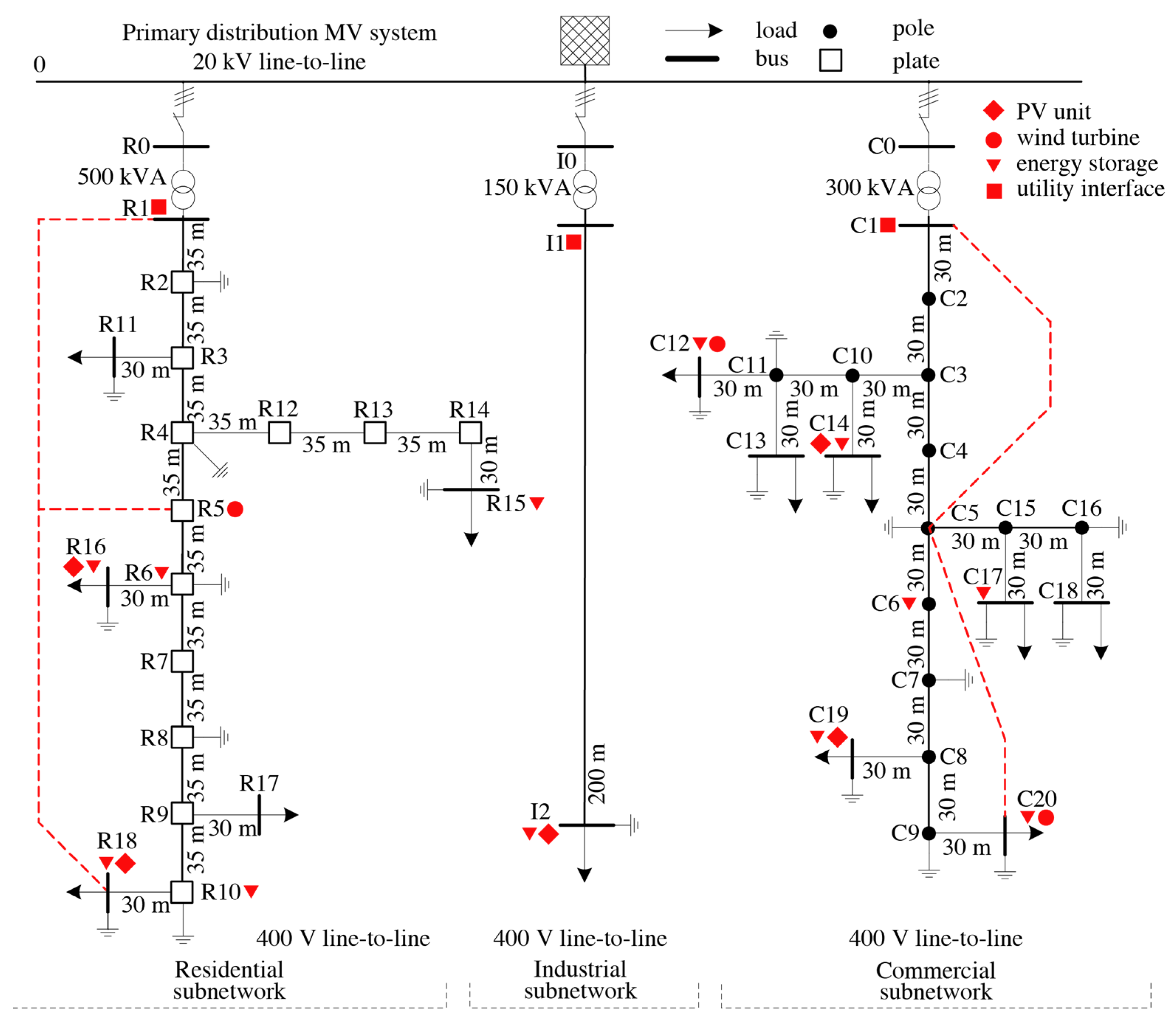
To analyze the operation and impact of the local control method proposed in the previous section, we consider the low-voltage microgrid shown in Figure 1, which corresponds to a European low-voltage benchmark network proposed by CIGRE [21]. This network has been already considered in a previous paper [13] and its configuration and parameters are recalled here for completeness.

The benchmark network includes three subnetworks: residential, commercial, and industrial. The characteristics and parameters of loads, sources, and distribution feeders are detailed in [13] and are reported in Appendix A. In particular,

Table A1. Parameters of the cables used in the application example in Figure 1.

Cable Type	Effective Area (mm2)	R Phase Wire (Ω/km)	L Phase Wire (mH/km)	R Neutral Wire (Ω/km)	L Neutral Wire (mH/km)	Rated Current (Arms)
UG1	240	1.63 × 10−1	4.33 × 10−1	4.90 × 10−1	1.50	430
UG2	150	2.66 × 10−1	4.81 × 10−1	7.33 × 10−1	1.81	325
UG3	120	3.26 × 10−1	5.03 × 10−1	8.60 × 10−1	2.01	290
UG4	25	1.54	6.56 × 10−1	2.33	4.63	120
UG5	35	1.11	6.21 × 10−1	1.93	4.03	145
UG6	70	5.69 × 10−1	5.54 × 10−1	1.29	2.75	215
OH1	50	3.87 × 10−1	9.39 × 10−1	6.89 × 10−1	1.50	172
OH2	35	5.24 × 10−1	9.77 × 10−1	8.38 × 10−1	1.56	145
OH3	16	1.15	1.05	1.84	1.69	93
I1	150	2.66 × 10−1	4.81 × 10−1	7.33 × 10−1	1.81	325

specifies the type of feeders;

Table A2. Details about the connections among grid nodes, the characteristics of the loads tied to the grid, and the parameters of MV/LV transformers feeding the three subnetworks considered in the application example in Figure 1.

Residential Subnetwork					Commercial Subnetwork					MV/LV Transformers (Yn)
Line	Node from	Node to	Length (m)	Cable Type	Line	Node from	Node to	Length (m)	Cable Type	Name	Node from	Node to	kVA	Vcc
R1	R1	R2	35	UG1	C1	C1	C2	30	OH1	RT	R0	R1	500	5%
R2	R2	R3	35	UG1	C2	C2	C3	30	OH1	CT	C0	C1	300	6%
R3	R3	R4	35	UG1	C3	C3	C4	30	OH1	IT	I0	I1	150	2%
R4	R4	R5	35	UG1	C4	C4	C5	30	OH1	Residential loads
R5	R5	R6	35	UG1	C5	C5	C6	30	UG6	Node	kW	kVAr	Conn	Random term vs. CIGRE profile
R6	R6	R7	35	UG1	C6	C6	C7	30	OH2	R11	13	8	Yn	±40%
R7	R7	R8	35	UG1	C7	C7	C8	30	OH2	R15	60	38	Yn	±40%
R8	R8	R9	35	UG1	C8	C8	C9	30	OH2	R16	46	30	Yn	±40%
R9	R9	R10	35	UG1	C9	C3	C10	30	OH2	R17	4.25	2.65	3n	±40%
R10	R3	R11	35	UG4	C10	C10	C11	30	OH2	R18	40	25	Yn	±40%
R11	R4	R12	35	UG2	C11	C11	C12	30	OH3	Commercial loads
R12	R12	R13	35	UG2	C12	C11	C13	30	OH3	C12	17	10.5	Yn	±30%
R13	R13	R14	35	UG2	C13	C10	C14	30	OH3	C13	6.8	4.2	Yn	±30%
R14	R14	R15	30	UG3	C14	C5	C15	30	OH3	C14	21.5	13	Yn	±30%
R15	R6	R16	30	UG6	C15	C15	C16	30	OH3	C17	13.5	8.5	Yn	±30%
R16	R9	R17	30	UG4	C16	C15	C17	30	OH3	C18	6.8	4.2	Yn	±30%
R17	R10	R18	30	UG5	C17	C16	C18	30	OH3	C19	21.5	13	Yn	±30%
Residential subnetwork meshing					C18	C8	C19	30	OH3	C20	17	10.5	Yn	±30%
R18	R1	R5	140	UG1	C19	C9	C20	30	UG4	Industrial loads
R19	R5	R18	200	UG1	Commercial subnetwork meshing					I2	60	37	Yn	20%
Industrial subnetwork					C20	C1	C5	120	UG1
I1	I1	I2	200	UG2	C21	C5	C20	150	UG1

shows the connections among grid nodes, the characteristics of the loads fed by the grid, and the parameters of the MV/LV transformers feeding the three subnetworks;

Table A3. Characteristics of the distributed energy resources considered in the application example in Figure 1.

Type	Node	Inverter Rating (kVA)	Rated/Max Power (kW)	Rated Energy (kWh)	Random Term vs. CIGRE Profile
PV unit	R16	55	4		±20%
	R18	50	3		±20%
	C14	25	20		±20%
	C19	25	20		±20%
	I2	80	20		±20%
Wind turbine	R5	7	5.5		±30%
	C12	25	20		±20%
	C20	25	20		±20%
Energy storage	R6	35	15/30	30
	R10	25	10/20	20
	R15	70	60/120	120
	R16	55	50/100	100
	R18	50	40/80	80
	C6	35	15/30	30
	C12	20	20/40	40
	C14	25	20/40	40
	C17	15	15/30	30
	C19	25	20/40	40
	C20	20	17.5/35	35
	I2	80	60/120	120
Utility interface	R1	120	50/100	100
	C1	120	50/100	100
	I1	80	35/70	70

specifies the characteristics of distributed energy sources.

As compared to the CIGRE benchmark network, wind turbines (WT, indicated by circular marker), photovoltaic systems (PV, diamond marker), and distributed energy storage systems (ESS, triangular marker) similar to those proposed for the residential subnetwork were added in the commercial and industrial sections, too. Moreover, energy storage units have been added as indicated in Figure 1 to allow the implementation of electrical safety procedures and extended local control. All distributed power sources, either RES (renewable energy sources) or ESS, interface to the grid by an electronic power converter that performs as a controllable current source. A special function is assigned to the utility interfaces (UI, square marker) located next to the points of common coupling (PCC) of each subgrid. They include ES units interfaced with the grid by voltage-controlled inverters and perform as voltage-tracking units during on-grid operation, and as voltage-forming units during off-grid operation. UIs play a fundamental role in controlling the power flow from and to the mains and are the basic elements to manage islanding and demand response and to handle transient situations due to faults or fast variations of network behavior.

The ESS located at nodes R6 and C6 are community units and support the UIs during fast transients. Under normal operation, they play as reactive and unbalance compensators according to the control methods described in the following sections.

To complement the CIGRE network, we also included the connecting lines shown in red color, which transform the original radial topology of each subnetwork to a meshed one. In practice, this corresponds to double the main power cable in the cable duct.

As discussed in a previous paper [13], choosing a meshed topology offers considerable advantages in the case of low-voltage microgrids: (i) the voltage stability at grid nodes improves; (ii) the power loss in distribution feeders reduces; (iii) faulty lines can be isolated without shutting down entire subgrids. Moreover, if a faulty area is surrounded by active nodes equipped with grid-tied inverters, the faulty currents can also be cleared by a proper control of the inverters, without opening the circuit breakers (electronic fault clearing). The faulty lines can then be isolated by opening disconnectors or by removing fuses. The same approach can be followed to isolate subgrids for maintenance.

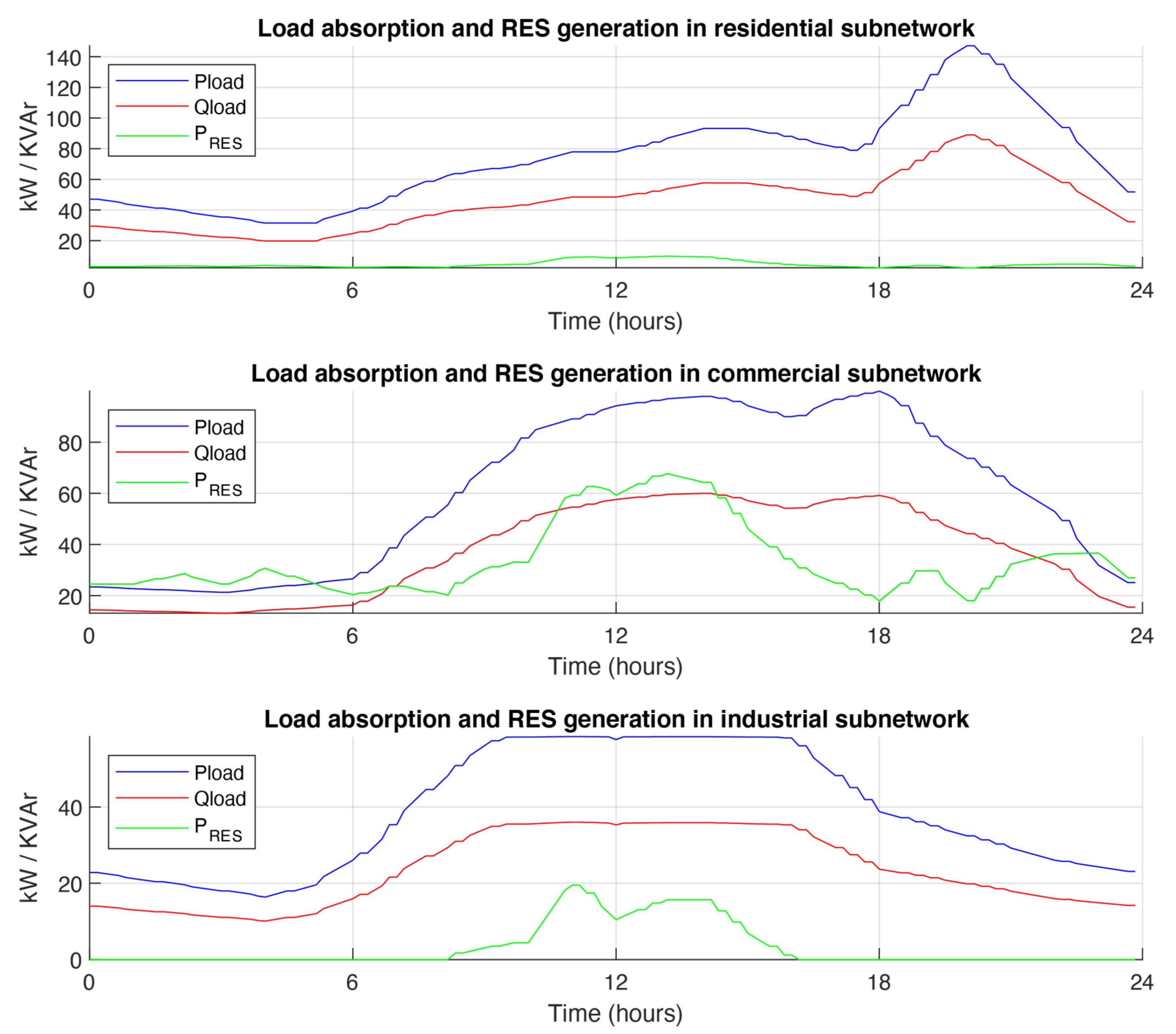
3.2. Daily Power Profiles

Figure 2 shows typical daily power profiles of the three subgrids of Figure 1, according to CIGRE standards for residential, commercial, and industrial microgrids in Europe.

The upper diagram shows the daily behavior of residential loads (active and reactive power absorption) together with the generation profile of renewable energy sources. The central and lower diagrams show the same quantities for the commercial and industrial subgrids, respectively. While the residential part is characterized by higher load power absorption, renewable energy generation is more relevant in commercial and industrial parts.

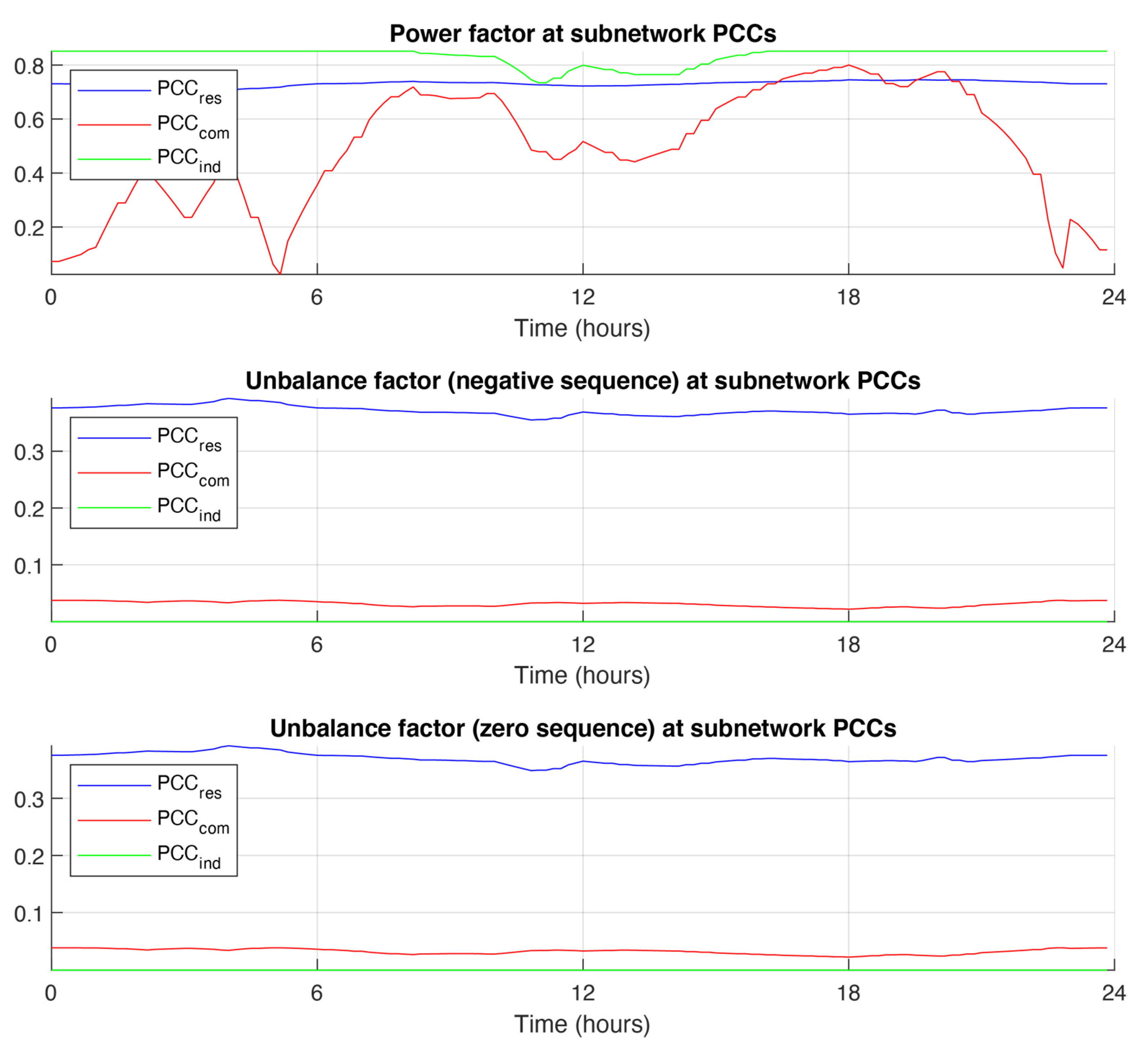
3.3. Mathematical Definition and Computation of Performance Factors

Figure 3 shows the daily behavior of three specific performance factors measured at the points of common coupling (PCCs) between each subgrid and the mains. Before discussing the behavior of such factors, let us introduce their mathematical definition and physical meaning in general terms.

In three-phase systems under periodic operation, the power factor (PF) is generally defined as:

$$PF=\frac{P}{A}=\frac{\langle \mathit{v},\mathit{i}\rangle }{\Vert \mathit{v}\Vert ·\Vert \mathit{i}\Vert }$$

(4a)

where $\mathit{v}$ and $\mathit{i}$ are the vectors of phase voltages and currents at a given network port, P is the active power flowing through that port, and A is the corresponding apparent power. The mathematical operator 〈·〉 indicates internal product, while ‖·‖ refers to the square norm (i.e., L² norm). In the time domain, for three-phase systems the power factor can be computed as:

$$PF=\frac{P}{A}=\frac{{\sum }_{k=1}^3{\int }_0^T v_k i_{k}dt}{\sqrt{{\sum }_{k=1}^3{\int }_0^T v_k^2 dt} ·\sqrt{{\sum }_{k=1}^3{\int }_0^T i_k^2 dt}}$$

(4b)

where $T$ is the line period, and $\left(v_k, i_k\right)$ indicate instantaneous phase quantities. Under sinusoidal operation, the PF can be computed as a function of RMS voltages and current as:

$$PF=\frac{P}{A}=\frac{{\sum }_{k=1}^3\left(V_k·I_k·\cos {\phi }_k\right)}{\sqrt{{\sum }_{k=1}^3{V}_k^2} ·\sqrt{{\sum }_{k=1}^3{I}_k^2}}$$

(4c)

where $\left(V_k, I_k\right)$ are the RMS voltage and current in phase k, and ${\phi }_k$ is their angular shift.

Equation (4c) can also be rewritten as a function of the sequence components of phase voltages $\left(V_p,V_n,V_o\right)$ and currents $\left(I_p,I_n,I_o\right)$. Owing to the orthogonality of the sequence terms defined by Equations (1)–(3), from (4c) we derive:

$$\begin{array}{c}PF=\frac{P}{A}=\frac{{\sum }_{k=1}^3\left(V_k·I_k·\cos {\phi }_k\right)}{3\sqrt{V_p^2+V_n^2+V_o^2} ·\sqrt{I_p^2+I_n^2+I_o^2}}\\ \hspace{1em}\hspace{1em}\hspace{1em}\hspace{1em}\hspace{1em}\approx \frac{{\sum }_{k=1}^3\left(V_k·I_k·\cos {\phi }_k\right)}{3V_p ·\sqrt{I_p^2+I_n^2+I_o^2}}\end{array}$$

(4d)

Equation (4d) clearly shows the impact on the power factor caused by reactive power absorption, which affects angular shifts ${\phi }_k$, and the asymmetrical behavior of phase currents, generated by the load unbalance, which may cause non-negligible negative and zero sequence terms $I_n,I_o$ to appear. In contrast, the impact of voltage asymmetry is usually minimal, since the negative- and zero-sequence voltage components at PCCs are negligible as compared to the positive sequence term.

The other two performance factors of Figure 3 describe the current asymmetry (power unbalance) measured at the PCCs, and are defined as:

$$\mathrm{Unbalance} \mathrm{factor} (\mathrm{negative} \mathrm{sequence}): {\chi }_n=\frac{I_n}{I_p}$$

(5a)

$$\mathrm{Unbalance} \mathrm{factor} (\mathrm{zero} \mathrm{sequence}): {\chi }_o=\frac{I_o}{I_p}$$

(5b)

• ${\chi }_n$ reflects the presence of unbalanced power absorption in the supply cables at the PCCs, and it is mainly due to asymmetrical single-phase loads connected line-to-line or line-to-neutral.
• ${\chi }_o$ reflects the presence of current circulation in the neutral wire, mainly due to single-phase loads connected line-to-neutral.

As mentioned before, the impact of voltage asymmetry is negligible and is not considered in our computation.

3.4. Performance Factors at PCC

Figure 3 shows the behavior of the above performance factors measured at the PCCs for the power profiles shown in Figure 2.

The upper diagram shows the daily behavior of the power factor, separately for each subgrid, while the central and lower diagrams depict the behavior of unbalance factors.

• The PF behavior of the residential subgrid is nearly constant along the 24 h interval. This regular profile reflects, on one side, the limited impact of renewable energy generation as compared to load power absorption and, on the other side, the fact that the power factor of residential loads keeps nearly constant at all times. Consequently, the ratio between active power P and apparent power A at residential PCC shows limited variations. Its relative low value (nearly 0.7) is mostly determined by the significant load unbalance, which derives from single-phase loads connected line-to-neutral and causes relevant unbalance factors (nearly 40% for both negative and zero sequence terms).
• The PF behavior of the commercial subgrid shows considerable variations, which are mainly determined by the irregular load power absorption, very low during the night, and by the impactful generation of renewable energy during daytime (both factors affect the ratio $P/A$). In contrast, in this subgrid the effect of load unbalance is limited, thanks to the significant amount of power absorbed by three-phase symmetrical loads.
• Finally, the industrial subgrid reveals a relatively high PF at all times, due to the coincidence of high-power absorption and generation during daytime, and low-power absorption and generation during nighttime. The unbalance factors are always negligible since almost every load is symmetrical in the three phases.

4. Local Control Methods and Their Impact on Performance Factors

In this section, we discuss two types of control approaches.

The first approach, called autonomous control, is applicable to each inverter tied to the grid without requiring any communication with other units or the grid manager. It only requires a modification of the inverter control firmware and the measurement (or estimation) of the active and reactive power absorbed by local loads (connected to the same grid terminals of the inverter), with a possible extension to surrounding loads.

The second approach, called cooperative control, implies the coordination of a group of inverters acting in the same subgrid. This method requires: (i) Collection and sharing of data on the overall active and reactive power absorbed by the loads in the subgrid, separately for each phase; this can be done by load power measurement, or even by day-ahead forecast, that should be sufficiently precise and reliable for this type of control, which is inherently stable and does not significantly degrade the grid operation even in case of data inaccuracy; (ii) Defining a suitable power sharing criterion among the inverters; for this purpose, sharing coefficients based on the rated kVA of each inverter can be determined offline, with the double advantage of avoiding real-time computations and ensuring uniform exploitation of inverters’ capacity. Even this control method requires updating the control firmware of the inverters. Moreover, some communication ability is needed, which is, however, consistent with mandatory requirements of modern grid codes.

4.1. Autonomous Control

The reference operation mode of the microgrid (Mode 0) is that depicted in Figure 2 and Figure 3 and refers to the case when RES inverters feed to the AC grid just the active power produced by energy sources, without compensating the load reactive power or the power unbalance. Moreover, all energy storage units remain off.

We now consider three types of autonomous control, which correspond to different operating modes of the microgrid.

• Mode 1—Local reactive power compensation. In this case, each inverter compensates the reactive power absorbed by the local loads fed at the same grid terminals. This type of compensation can be implemented in single- and three-phase inverters.
• Mode 2—Local reactive power and unbalance compensation. In this case, each inverter compensates for the reactive power absorbed by local loads and for the negative- and zero-sequence currents generated by the asymmetry of these loads. While negative-sequence compensation is applicable to any type of three-phase inverter, zero-sequence compensation requires a connection to the neutral wire. With this type of control, every grid node equipped with a three-phase inverter can perform at unity power factor.
• Mode 3—Reactive power and phase unbalance compensation of vicinity loads. The previous control methods do not allow reactive and unbalance compensation of loads connected to passive grid nodes, i.e., not equipped with inverters. However, Mode 2 can be extended to the case where inverters receive information on the power absorption of vicinity loads and develop an aggregate compensating action. For example, in the network of Figure 1, we aggregate nodes R10 and R17, so that the inverter in R10 compensates for all loads at nodes R10 and R17. Similarly, we aggregate neighbor nodes R11 and R15, C12 and C13, C17 and C18.

4.2. Cooperative Control

Following the proposal introduced in Section 2.3.2 and further discussed at the beginning of this section, we may apply cooperative control to all inverters of each subgrid. The resulting operation mode is:

• Mode 4—Cooperative compensation in subgrids. In this case, we exploit the control ability of the utility interfaces, located next to each PCC, to strengthen the compensation action performed by the other inverters connected to the same subgrid.

4.3. Active Node Structure and Control Implementation

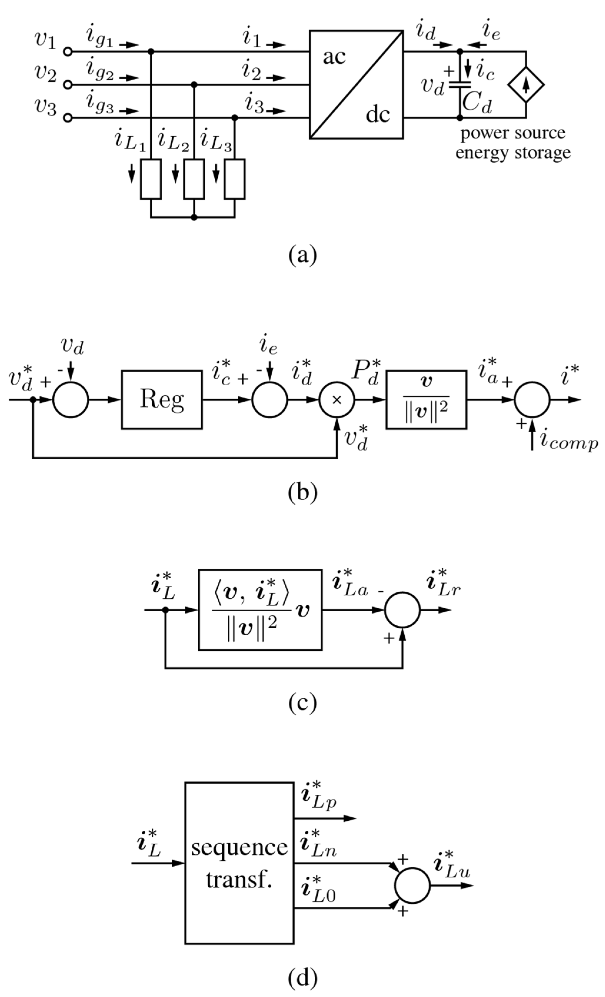
4.3.1. Active Node Structure

Figure 4a depicts the general structure of an active node, equipped with an AC/DC pulse-width-modulated (PWM) inverter interfacing the AC grid with the DC circuit. This latter generally includes a power source and/or energy storage unit in addition to filter capacitor $C_d$. AC loads can also be connected at the same grid terminals of the inverter. In Figure 4a we define:

• ${\mathit{i}}_g$, ${\mathit{i}}_L$, and $\mathit{i}$ as respectively the vectors of the total currents drawn from the AC grid, absorbed by the AC loads, and entering the inverter AC terminals;
• $v_d$ and $i_d$ as respectively the DC voltage and the current fed by the inverter to the DC link;
• $i_c$ and $i_e$ as respectively the current absorbed by DC filter capacitor $C_d$ and that fed by the DC source, either power source or energy storage unit.

4.3.2. General Control Principle

As known, PWM inverters allow a high flexibility to control the waveform of AC currents, under the constraint of input/output power balance and within the limits set by kVA power rating. All proposed control methods suit these boundaries, while taking full advantage of the control flexibility to impress the desired reactive and unbalance compensation currents. The general control principle is depicted in Figure 4b.

The main control loop refers to DC voltage $v_d$, since keeping $v_d$ at the reference value ensures the balance between inverter input and output power. Actually, any mismatch between these power terms would cause the energy in capacitor $C_d$ to increase or decrease, thus causing a variation of $v_d$. Fort this purpose, the voltage control loop adjusts the value of DC current $i_d$ which, in turn, reflects on the amplitude of the active currents entering the inverter.

This is graphically represented in Figure 4b, where the control amplifier $Reg$ adjust capacitor current reference $i_c^{*}$ to keep voltage $v_d$ at desired reference $v_d^{*}$. Inverter DC current reference $i_d^{*}$ is then determined by detracting source current $i_e$ from $i_c^{*}$. By multiplying DC voltage reference $v_d^{*}$ times DC current reference $i_d^{*}$ the control estimates DC power reference $P_d^{*}$ which, under the assumption of input/output power balance, also coincides with the AC active power reference $P_a^{*}$. Active ac current references ${\mathit{i}}_a^{*}$ are then determined as those quantities proportional to AC voltages $\mathit{v}$ which comply with power reference $P_a^{*}=P_d^{*}$. Finally, inverter AC current references ${\mathit{i}}^{*}$ are determined by adding compensation terms ${\mathit{i}}_{comp}$ to active current references ${\mathit{i}}_a^{*}$. Since reactive and unbalance compensation currents do not alter the active power flow, the inverter will eventually absorb the required active power while performing the compensation action required by the selected control method.

4.3.3. Determination of Reactive and Unbalance Compensation Currents

According to the above control methods, each inverter is required to compensate totally or partially the reactive and unbalance currents of one or more vicinity loads. The compensation duty assigned to each inverter depends on the selected control method and the power sharing criterion.

Assuming that ${\mathit{i}}_L^{*}$ is the vector of the equivalent load currents to be compensated by the inverter of Figure 4a, the control must firstly separate the active and reactive components of such currents. The separation procedure is shown in Figure 4c. The active components ${\mathit{i}}_{La}^{*}$ are first determined as those currents proportional to line voltages $\mathit{v},$ which convey the same active power of currents ${\mathit{i}}_L^{*}$. The reactive components ${\mathit{i}}_{Lr}^{*}$ are then determined by difference. If only a reactive compensation is required, compensation terms ${\mathit{i}}_{comp}$ of Figure 4b simply coincide with the opposite of equivalent load reactive currents ${\mathit{i}}_{Lr}^{*}$.

If unbalance compensation is also required, the control determines the sequence component of currents ${\mathit{i}}_L^{*}$ according to the transformation equations of Section 2.2. The procedure is depicted in Figure 4d, where negative-sequence term ${\mathit{i}}_{Ln}^{*}$ and zero-sequence term ${\mathit{i}}_{Lo}^{*}$ are added to determine total unbalance currents ${\mathit{i}}_{Lu}^{*}$. These latter terms are then accounted for in the computation of compensation term ${\mathit{i}}_{comp}$.

In the most general case of reactive and unbalance compensation, we set:

$${\mathit{i}}_{comp}=-{\mathit{i}}_{Lr}^{*}-{\mathit{i}}_{Lu}^{*}$$

(6)

Remarkably, the control relies on basic control functions at the inverter level. These consist of output active and reactive output power, which are foreseen in current grid standards [22] too, and inverse sequence current injection, which is a basic functionality widely discussed in the literature [23].

4.4. Impact of Control Methods on Grid Performance

• In this section, we analyze separately the performances of residential, commercial, and industrial subgrids, since their different characteristics facilitate the discussion on the impact of the various control techniques on overall microgrid operation.

4.4.1. Impact on the Power Factor of Commercial Subgrids

First, we analyze the effect of the above control methods on the power factor measured at the PCC of the commercial subgrid. We refer to this subgrid because of the large variations of its power factor shown in Figure 3.

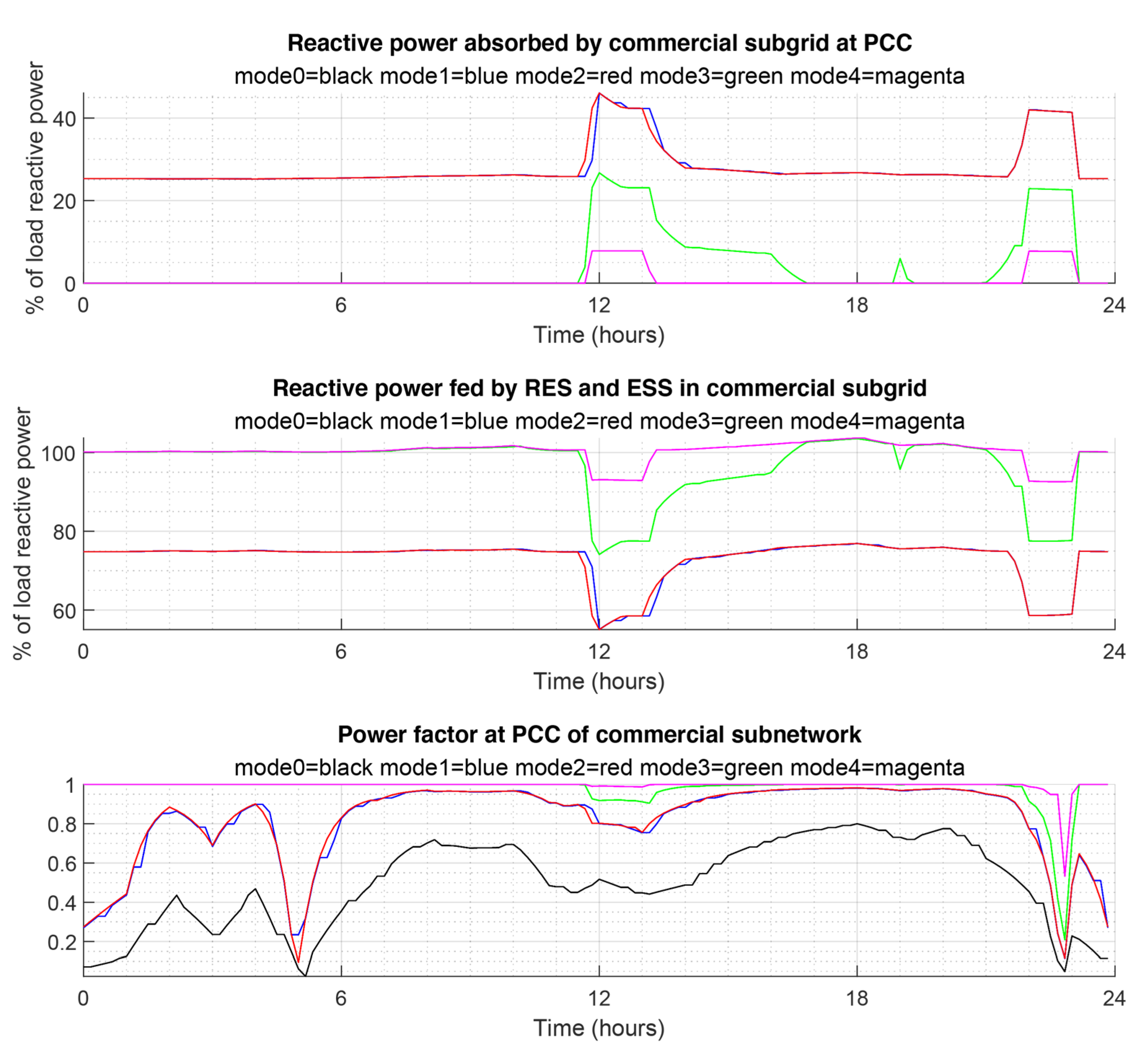
The results of the analysis are summarized in Figure 5.

• The upper diagram shows the time behavior of the reactive power fed by the mains at PCC for the various control methods. The values are expressed in percentage of the total reactive power absorption of the loads in the subgrid. In every operating mode, the reduction of the reactive power fed by the mains is impressive. In mode 1, the maximum value does not exceed 40% of load power, with an average of about 25%, and the same happens in mode 2. The reason for the similar behavior in modes 1 and 2 is that the reactive power fed by the inverters is the same in both cases (it coincides with the reactive power of local loads), the main difference being related to load unbalance compensation, which is a minor issue in commercial subgrids. Instead, modes 3 and 4 provide a greater reduction of reactive power absorption, since the aggregation of vicinity loads (mode 3) or the cooperative control within the entire subgrid (mode 4) allow much better compensation of the overall reactive power taken by the loads. Note that the compensation is less effective in the central hours of the day, where renewable energy generation is high, and in late afternoon, where load power absorption is maximum. In both cases the compensating action is limited by the kVA ratings of the inverters.
• The central diagram shows the corresponding behavior of the reactive power fed by the inverters within the subgrid, whose action is increasingly effective when adopting more sophisticated control methods. This diagram further clarifies that a full compensation of load reactive power is not possible even for mode 4 (cooperative control in the entire subgrid) in the central hours of the day. The reason is that in those hours the generation of renewable energy is maximum, thus the inverters are primarily committed to feed the active power produced by the sources and their residual capacity for load reactive power compensation is limited by the kVA ratings. In presence of an energy storage system, the flexibility of operation could obviously be extended, e.g., by temporarily storing the energy produced by the power sources to recover the full reactive power compensation ability.
• The lower diagram shows the effect of the various control methods on the power factor measured at the PCC. As compared to the reference situation of mode 0, the benefit is appreciable in modes 1 and 2, and is nearly ideal (unity power factor) in modes 3 and 4.

Overall, all proposed control methods allow significant improvements over the reference operating mode. In particular, the compensation of vicinity loads (mode 3) provides excellent performance without requiring the implementation of collective measurements or power sharing among inverters.

4.4.2. Impact on the Unbalance Factors of Residential Subgrid

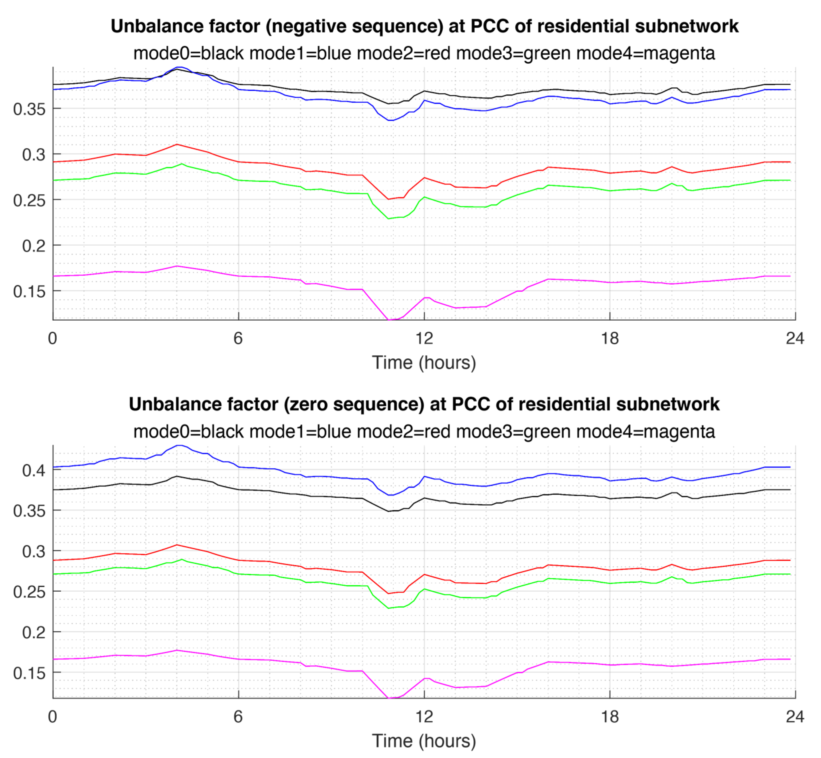
We now analyze the impact of the various control methods on the unbalance factors in the residential subgrid, which mostly suffers the effects of load unbalance. The results are summarized in Figure 6.

• The upper diagram refers to the behavior of the unbalance factor related to the presence of negative-sequence currents at PCC. As compared to the reference operation of mode 0, the pure reactive power compensation method of mode 1 does not reduce the unbalance factor. In fact, in this mode the inverters feed symmetrical reactive currents and do not substantially contribute to the elimination of negative-sequence components. The other operating modes perform significantly better, and the cooperative control of mode 4 reduces the unbalance factor to nearly one-third.
• The lower diagram refers to the behavior of the unbalance factor related to the presence of zero-sequence currents at PCC. As compared to the reference operation of mode 0, the pure reactive power compensation method of mode 1 slightly increases the unbalance factor. The reason lies in the symmetrical operation of the inverters, which increases positive-sequence currents without impacting on zero-sequence load unbalance. The other operating modes ensure increasingly appreciable reductions of the unbalance factors when switching from mode 2 to mode 3 to mode 4.

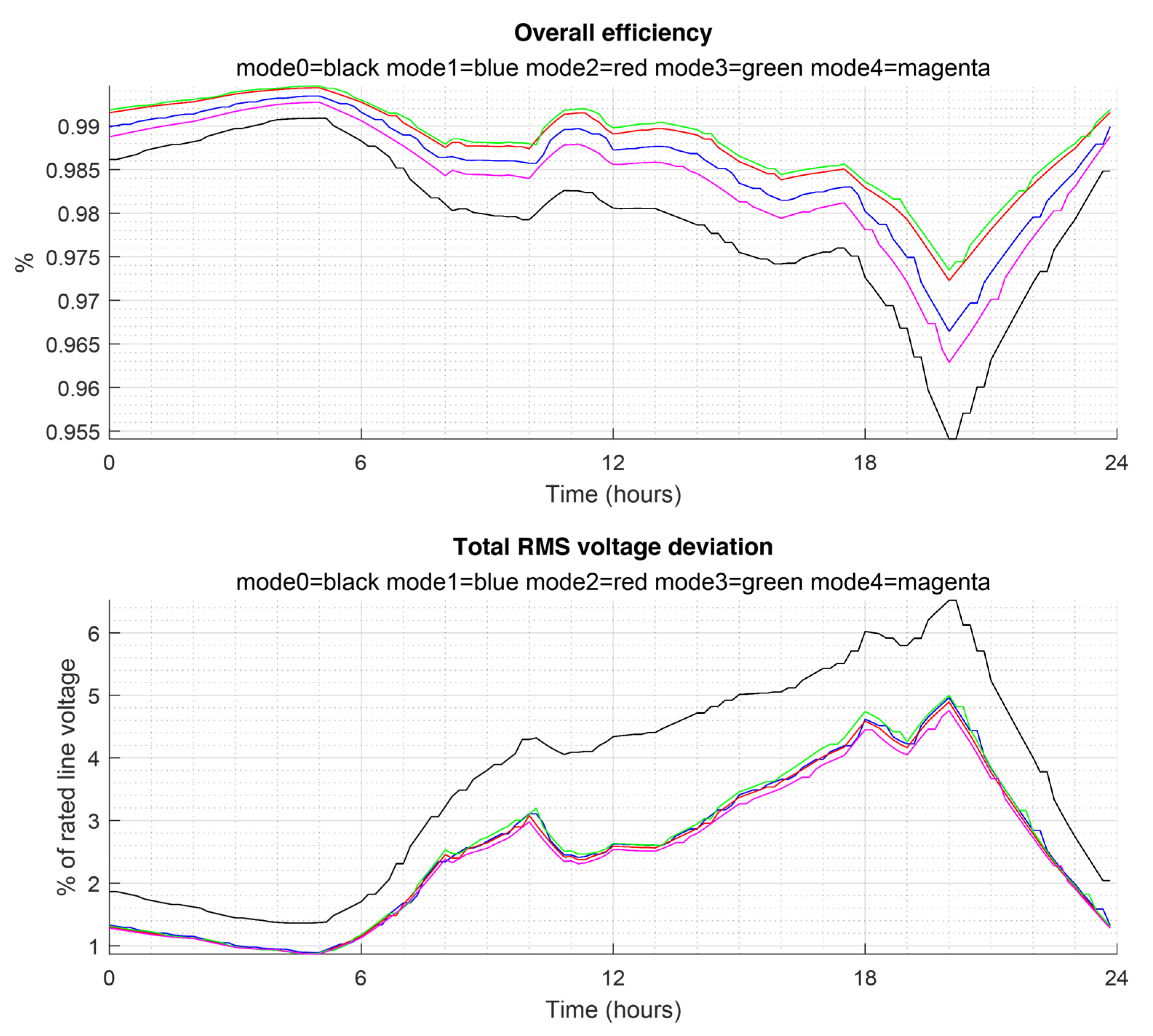
4.4.3. Impact on Overall Efficiency and Total Voltage Deviation

The overall efficiency is defined as:

$$\eta =\frac{P_{load}}{P_{fed}}=1-\frac{P_{loss}}{P_{fed}}=1-\frac{P_{transf}+P_{wires}+P_{inv}}{P_{PCC}+P_{gen}+P_{ESS}}$$

(7)

where $P_{load}$ is total power absorbed by the loads, and $P_{fed}$ is the total of the power fed by the mains at PCC ($P_{PCC}$) and that generated by the sources in the microgrid ($P_{gen}$, generated by any type of local power sources, and $P_{ESS}$ fed by ESS). $P_{loss}$ is total power loss, i.e., the sum of transformer power loss ($P_{transf}$), power loss in the distribution wires ($P_{wires}$), and inverter loss $P_{inv}$ (which accounts for internal losses of energy sources too).

The total voltage deviation is defined as:

$${\Delta }_v=\sqrt{\sum _{k=1}^N{\left(V_k-V_{nom}\right)}^2}$$

(8)

where N is the total number of grid nodes, $V_k$ is the RMS value of the voltage measured at node k, and $V_{nom}$ is the rated RMS grid voltage. Term ${\Delta }_v$ is a root-mean-square factor and gives a general indication on the steadiness of the voltage profiles across all nodes of the microgrid. As an alternative indicator, the minimum voltage across the entire microgrid can be considered.

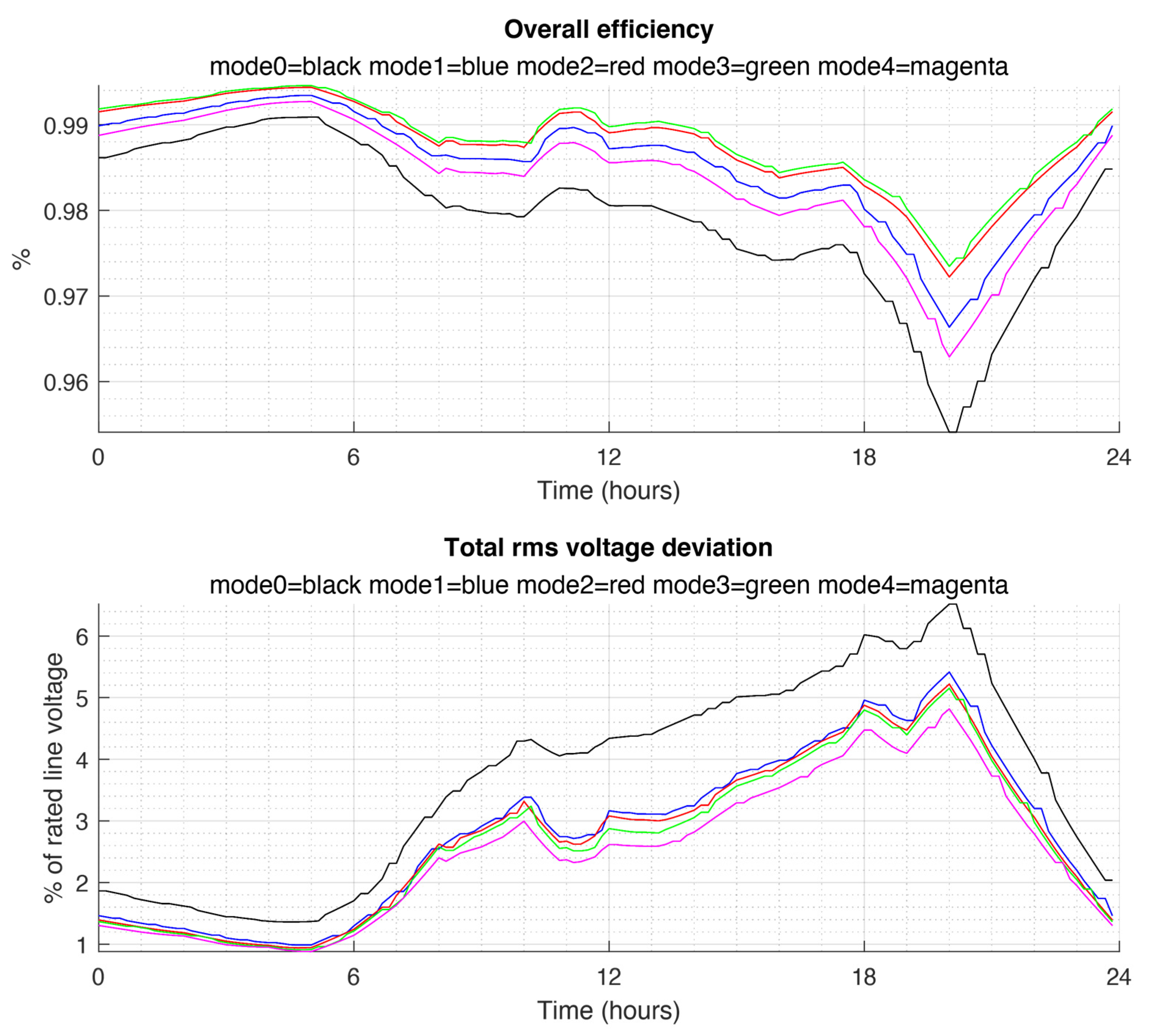
Figure 7 shows the time behavior of the overall efficiency $\eta$ and total voltage deviation ${\Delta }_v$ in the various operating modes. In all cases, the improvement over the reference situation of mode 0 is appreciable.

• The upper diagram shows that the efficiency is generally higher for modes 2 and 3, due to the local elimination of useless current terms (reactive currents and negative/zero-sequence components), which do not flow through the grid wires toward the PCC. In mode 1 this happens partially, since only the reactive power absorbed by the loads is compensated locally. Instead, mode 4 is characterized by additional losses since the circulation of compensating currents happens through longer paths than for modes 2 and 3. As compared to reference operation mode 0, where inverters do not perform any compensation actions, all proposed control methods provide considerable efficiency improvements along the entire time period.
• The lower diagram shows that all control methods ensure a reduction of the total voltage deviation as compared to the reference situation. This happens because the local compensation of reactive and unbalance power prevents circulation of useless reactive and unbalance current terms, thus reducing the voltage drop across the grid wires.

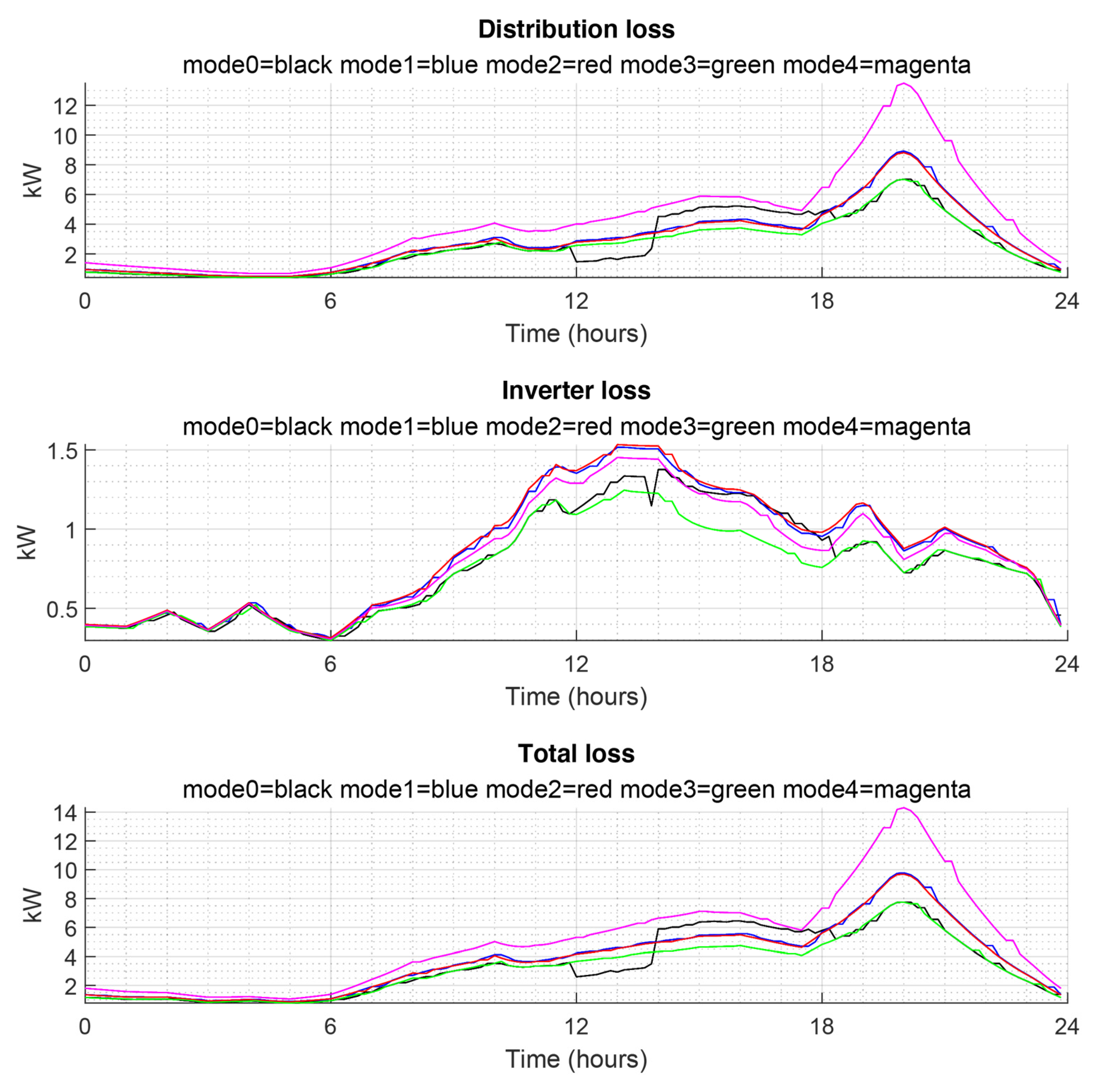
It is also interesting to see how the distribution and inverter losses change during the time for the various control methods. This is shown in Figure 8, where the upper diagram refers to distribution losses, which essentially track the behavior of load power and slightly increase in case of cooperative control, where the compensation currents flow though longer paths. The lower diagram refers to conversion losses, which increase in the central hours of the day, where the power fed by renewable sources is maximum. Note that the adoption of cooperative control methods helps to reduce the inverter losses, thanks to power sharing. It must also be observed that the diagram was drawn assuming inverters with an efficiency above 94%, which is consistent with, for example, [24].

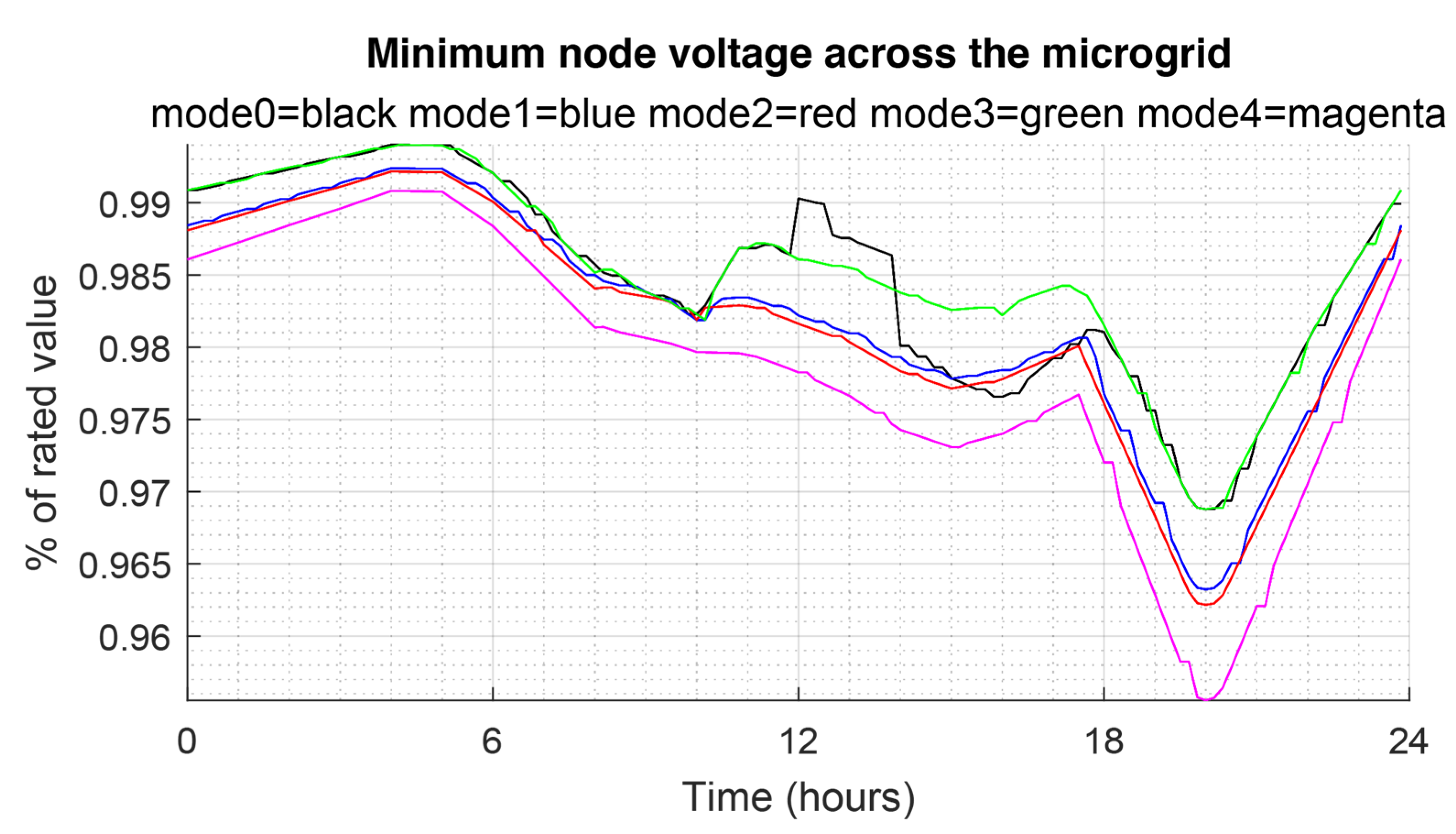
Finally, Figure 9 shows the minimum node voltage measured across the entire microgrid for the various control methods. Noticeably, while local compensation of vicinity loads helps the steadiness of voltage profiles, the requirement of unity power factor at PCCs affects it, since reactive and unbalance currents flow through the microgrid, causing additional voltage drops along the distribution lines.

Overall, the proposed local control modes show the ability to reduce the power loss and stabilize the voltage profiles within the entire microgrid.

5. Integrating Local Control and Central Control

As mentioned in Section 2.3.3, the above local control methods can profitably be integrated with centralized control to extend the operational limits of the microgrid. Here we consider an integration approach that does not require any modifications of the above reactive and unbalance compensation techniques conducted at a local level.

Rather, we extend the same local control approach to include active power too, assuming that local energy storage units can be driven to temporarily compensate (e.g., to accomplish islanding or demand response) for the active power absorbed by their vicinity loads. This operation mode is toggled on or off by a logical command issued by the central controller, without any additional data exchange with local units.

The only units requiring bidirectional communication with the central controller are the utility interfaces, which interact with the grid manager to implement additional functions such as demand response or islanding.

5.1. Integration of Local and Central Control for Reactive Power and Load Unbalance Compensation

For the sake of demonstration, let us assume that the compensation functions described in the previous chapter are integrated with a power factor control action done by the UIs under the guidance of central control. For this purpose, the information on the reactive and unbalance currents absorbed at the PCC are fed by the central controller to the UIs, which adapt their operation to provide the residual compensation needed to complement that performed by local control methods. The result is a unity power factor operation at all PCCs irrespective of the type of local control used by the inverters in the microgrid. This means that at any time the currents fed by the mains are purely active, symmetrical, and in phase with the line voltages. This means that all reactive and unbalance currents taken by the loads are compensated within the microgrid, without affecting the mains.

To verify that the integrated control does not affect the overall efficiency and voltage stability at grid nodes, Figure 10 shows the same quantities of Figure 7 when the UIs are driven by central control. Noticeably, the voltage deviation factor is substantially unaffected, while the overall efficiency is further improved. It is also remarkable that the highest efficiency is achieved by implementing locally the simplest control technique (mode 2), where the inverters compensate for local loads only, without requiring data exchange with other units in the same subgrid.

This demonstrates that driving the UIs by central control may ensure nearly ideal operation at the PCCs, high efficiency, and steady voltage profiles without requiring data sharing among the inverters in the same subgrid.

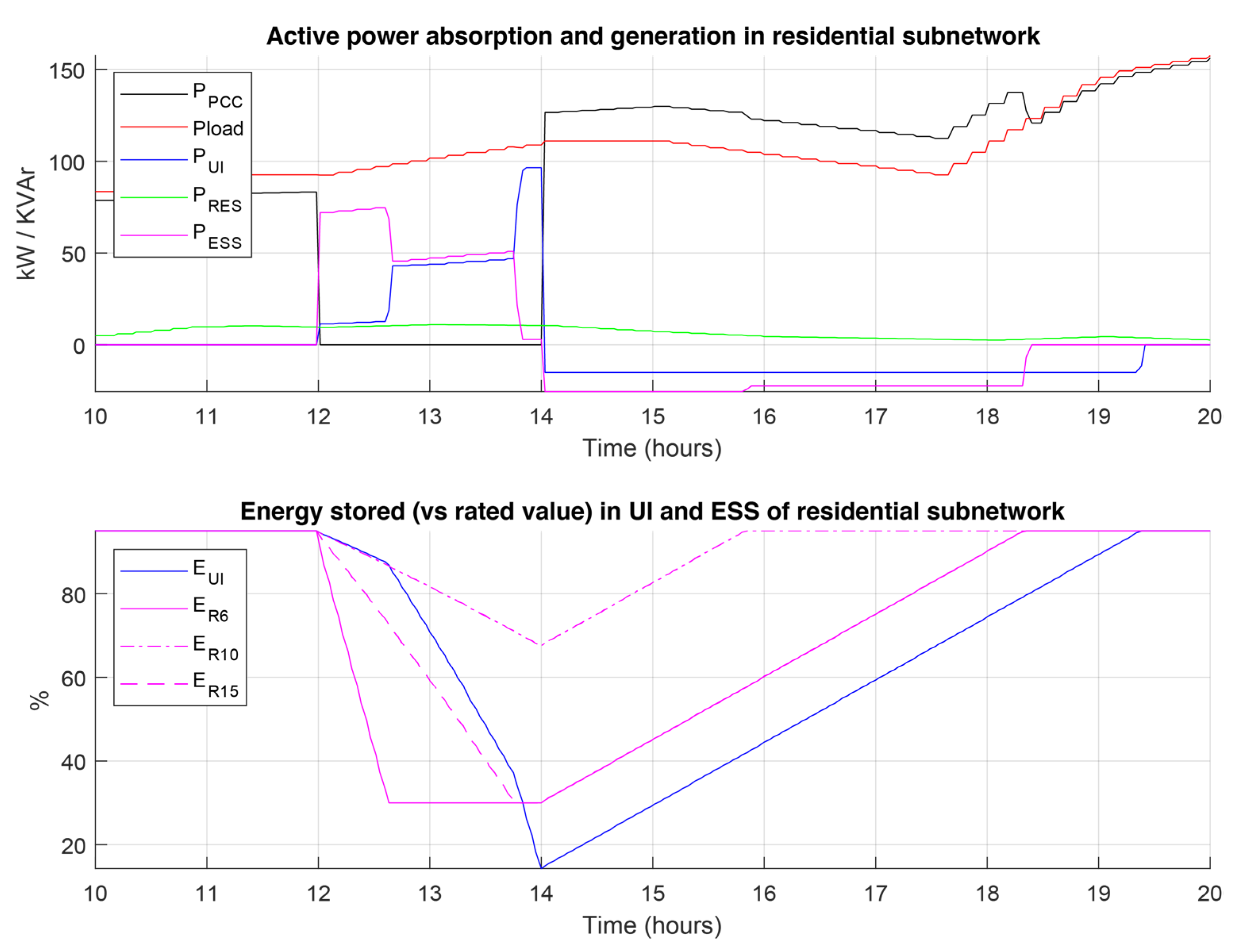
5.2. Integration of Local and Central Control for Active Power Management in Case of Islanding

The integration of local and central control has the potential to allow a precise management of the power flowing at the PCCs, making possible the implementation of demand response, or even islanding of entire subnetworks. For the sake of demonstration, we consider the case when, in the time interval from 12 a.m. to 2 p.m., the residential subgrid is driven in the islanded mode, while in the remaining time the operation remains in mode 4.

The corresponding time behavior of some relevant quantities of the residential subgrid is shown in Figure 11.

At 12 a.m. the active power compensation command is issued to all nodes equipped with energy storage (R6, R10, R15), and each unit suddenly begins to feed the active power requested by the associated loads (loads R16 and R18 for R6; load R17 for R10; loads R11 and R15 for R15). The UI at node R1 receives data measured at PCC and arranges its output currents to compensate for the residual active and reactive power and unbalance factors.

At 2 p.m. the islanding condition is removed, and the energy storage units enter a charge recovery phase at constant current. At 7.30 p.m. this phase also ends and the operation returns to regular mode 4.

• The upper diagram shows the active power: fed by the mains at PCC (black line); absorbed by all loads in the subgrid (red); fed by the utility interface at node R1 (blue); generated by the renewable energy sources in the microgrid (green); fed by the energy storage units at nodes R6, R10, and R15 (magenta).
• The lower diagram shows the behavior of the energy stored in the ES units at node R1 (UI, blue line), R6 (magenta, continuous), R10 (magenta, dash-dotted), R15 (magenta, dashed).

We observe that before 12 a.m. the load power is fed by the mains at PCC and by RES only. After the islanding command is issued at 12 a.m., the power fed at PCC vanishes, and the corresponding power gap is quickly filled by UI and ES units. Most of the power is initially fed by ES units, until at 12.30 a.m. the unit at R6 reaches the minimum charge limit (30% of rated value) and stops feeding power. The UI steps up suddenly to fill the gap, and further increases its power contribution at 1.30 p.m., when the ES in R10 also reaches the lower charge limit. At 2 p.m. the UI’s energy is nearly exhausted (15% of rated value) and the islanding phase ends. In the following hours the storage units recover the full charge at constant current, and the mains feeds the load power plus the energy recovery power of ES units. At 7.30 p.m. the energy recovery phase is completed and the system returns to mode 4 (unity PF at PCC).

Note that, even for this type of operation, the local units operate autonomously based on local power data. The required active power control can be implemented by upgrading the control firmware to include the on/off toggle for load power compensation.

6. Discussion

In this paper, we proposed a control approach that can be applied for retrofitting existing grid-tied inverters with the aim of improving their individual operation as well as the performance of the surrounding grid.

In particular, three types of control were discussed, which are characterized by different performances but require only handling of the power and current data measured locally:

• With the simplest type of control, the inverters are driven to compensate the total reactive power absorbed by the loads fed at the same grid terminals of the inverter. This only requires a revision of the control firmware and local reactive power measurements. This type of control prevents useless reactive power terms flowing through the distribution feeders, resulting in reduced distribution loss and limited fluctuations of the voltages at grid nodes.
• In the case of three-phase inverters, the above approach can be extended to the compensation of the power unbalance generated by local loads. This requires a more sophisticated control algorithm in the inverter control firmware; moreover, local phase power and currents must be measured to allow computation of negative- and zero-sequence terms. The result is an increase in the computational burden of each inverter which, however, keeps well within the capability of commercial controllers. The corresponding performance improvement is very appreciable in terms of power factor at the point of common coupling since the symmetry and phase shift of the currents fed by the mains significantly improve. The overall efficiency also increases, since most useless current terms are prevented from flowing in the distribution feeders. For the same reason also, the voltage profiles improve since the asymmetrical voltage drops caused by the circulation of negative- and zero-sequence currents are attenuated.
• A further extension is achieved if each inverter performs reactive and unbalance compensation for a set of vicinity loads. The control algorithm is the same as in the previous case; however, the range of measurement extends to cover neighbor loads.

Two additional control methods have been considered, which further improve the performances but require data sharing among the inverters and/or interaction between the central control and the utility interfaces:

4.

The first method coordinates all inverters of a subgrid to compensate for the total reactive power absorption and load unbalance generated within the subgrid. While providing excellent performances, this method requires data exchange within the subgrid and the implementation of suitable power sharing criteria among the inverters. Correspondingly, its implementation is more complex and demanding than for the previous cases.

The second solution requires the implementation of the simple control method mode 2 in all inverters but the utility interfaces. These latter receive data on total power absorption from the central controller. Correspondingly, each UI computes and compensates for any residual reactive and unbalance power terms in the subgrid. The results are unity power factor at the PCCs, high efficiency and voltage stability, without overstressing the UI inverters, which are supported by any other inverters in the same subgrid.

Overall, the simplicity of control is appreciable as compared to that of solutions based on centralized or distributed optimum or consensus-based control techniques, which may require dynamic and adaptive control algorithms and high-frequency communication of ubiquitous data collected by fast meters. Even though the considered methods are presented referring to steady-state considerations, they are also effective with typical load and generation dynamics, as shown by the time-varying 24 h profiles considered in the presented case studies. In addition, the response in case of the occurrence of fast transients of similar control algorithms has been already analyzed considering realistic conditions; for example, in [25], showing that no significant impact occurs on the main microgrid performances.

Notably, the control methods presented in this paper do not suffer from potential instability, since the interaction among inverters is minimal; in fact, the limited voltage variations occurring during normal operation of the grid do not substantially affect the control methods presented here.

Finally, we observe that the proposed control performs properly even in case of measurement inaccuracy or estimation error, since moderate control errors by local inverters do not affect significantly the overall efficiency and voltage stability of the network. In any case, the performances at PCCs can be adjusted by corrective actions done by the utility interfaces.

7. Conclusions

The establishment of energy communities as active players in the energy market requires the capacity to handle the energy resources in a coordinate way. This is the basis for energy trading, whose reward may justify collective efforts to strengthen the facility and improve the effectiveness and resilience of energy management.

Microgrids represent the most viable solution to aggregate neighboring end users who share their resources for mutual benefit. Exploiting the full potential of such aggregations, however, requires smart control and coordination of energy resources, which may be difficult if the inverters tied to the distribution grid are not equipped with flexible control and communication.

To circumvent this limit, we presented some methods of local control which do not require communication and can be implemented even in existing inverters by updating their control firmware.

We also discussed more advanced solutions, which rely on community energy storage units, equipped with flexible control and communication interfaces, and permit control of the power flow at the points of common coupling with the mains.

The application of the proposed control methods to a benchmark network demonstrated that even pure local control techniques can significantly improve the quality of operation of the microgrid from several perspectives, e.g., energy efficiency, voltage steadiness, and power unbalance. It was also shown that integrating local and central control makes possible more sophisticated and rewarding interaction with the mains, including demand response and islanding.

Overall, it seems that several planned benefits of energy communities can be achieved without substantial renovation of existing infrastructure and equipment. In fact, retrofitting existing plants and establishing community energy storage systems would provide a wide set of operational tools to control and trade energy in the wholesale market.