
Optimal Design of PV Inverter Using LCOE Index †

 ,
, 
Abstract
:1. Introduction
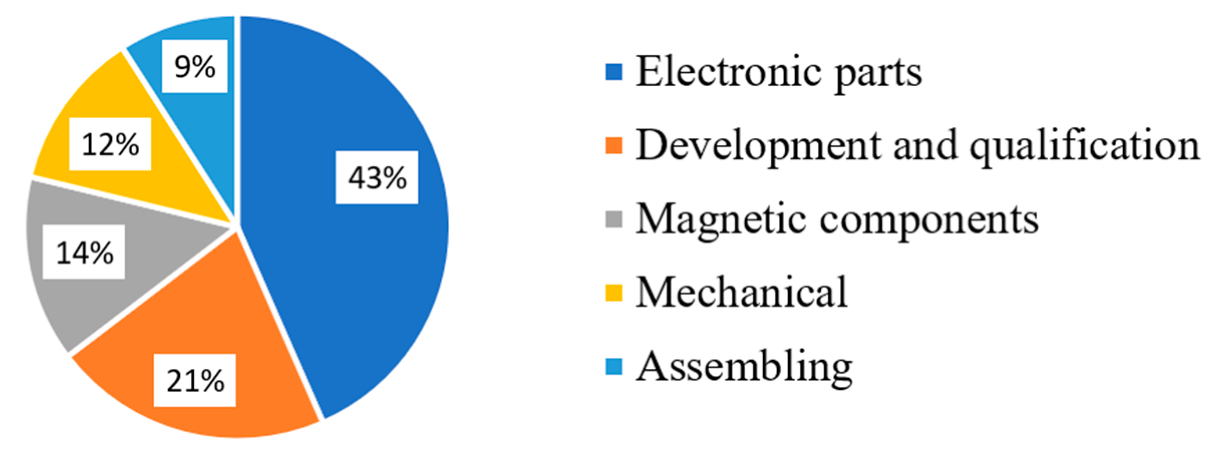
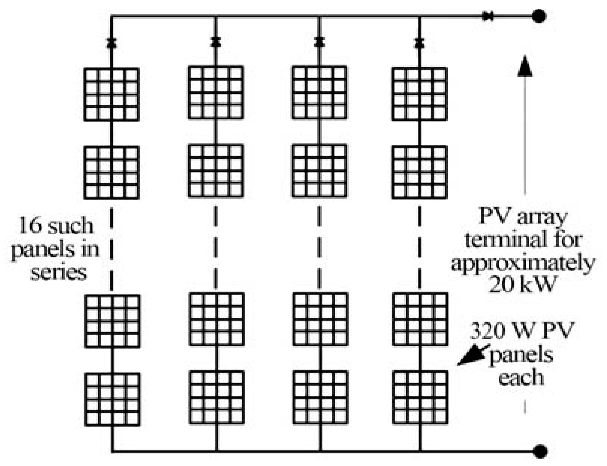
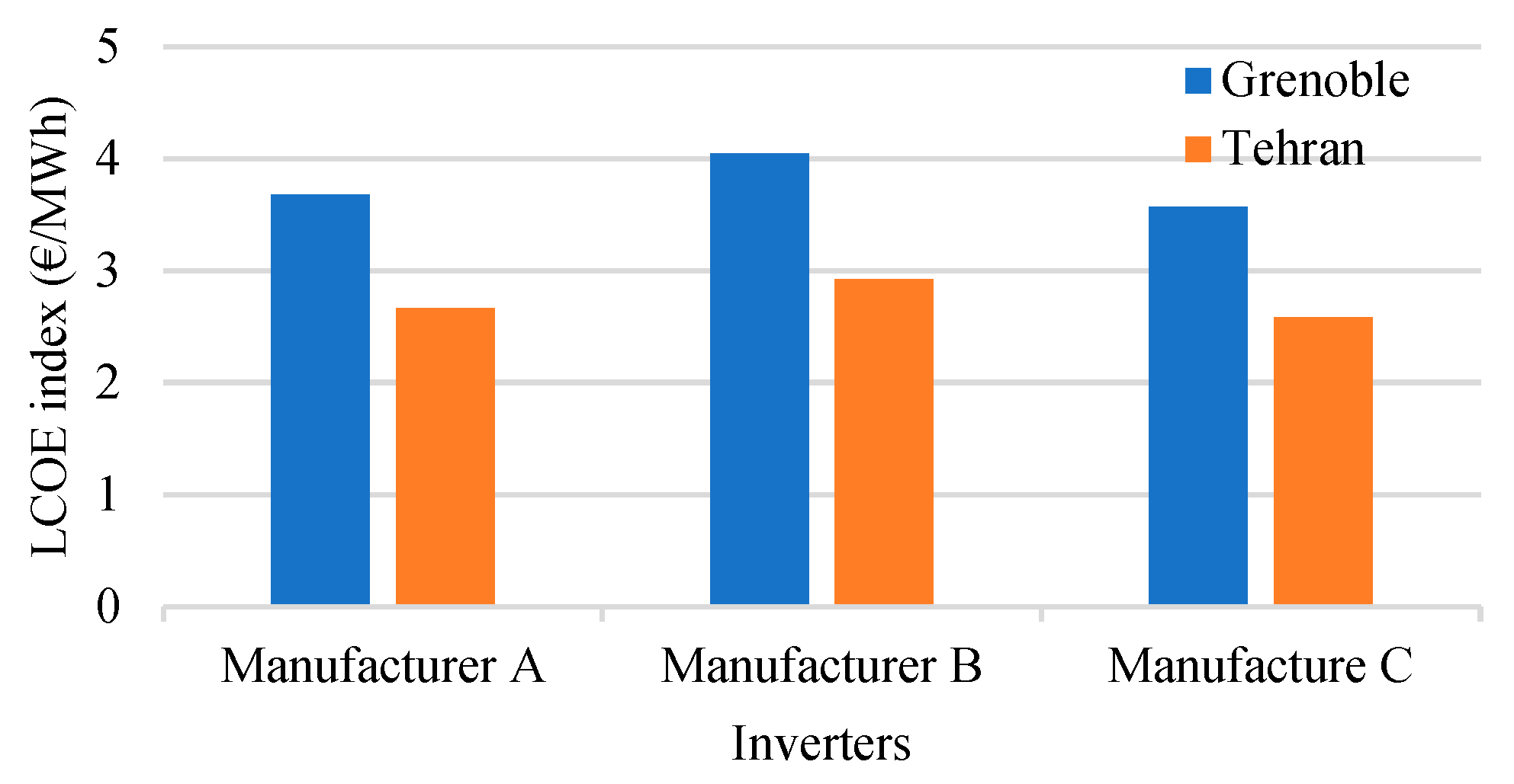
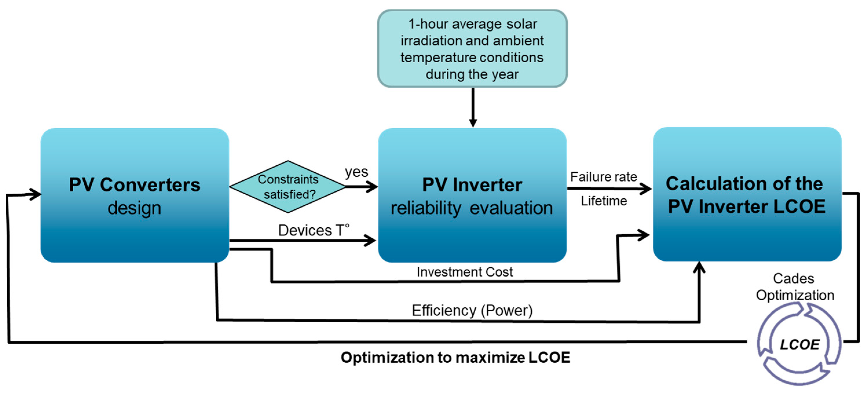
2. LCOE of Industrial Inverters: Case Study
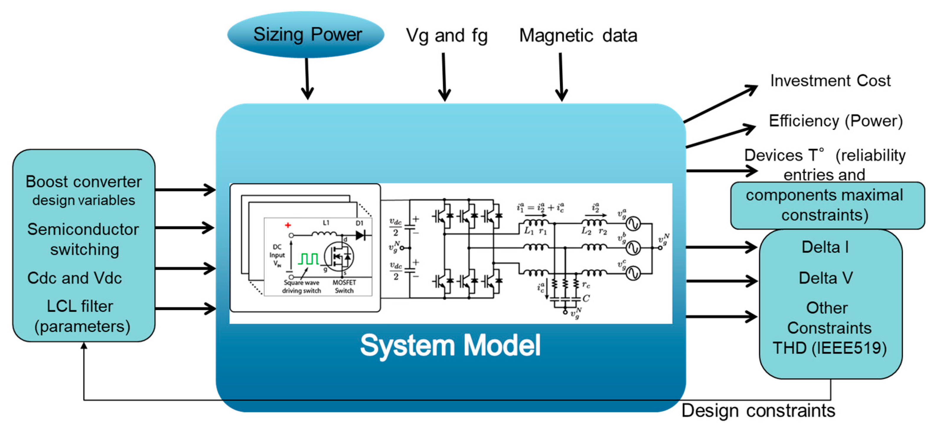
3. Models for Inverter Pre-Sizing
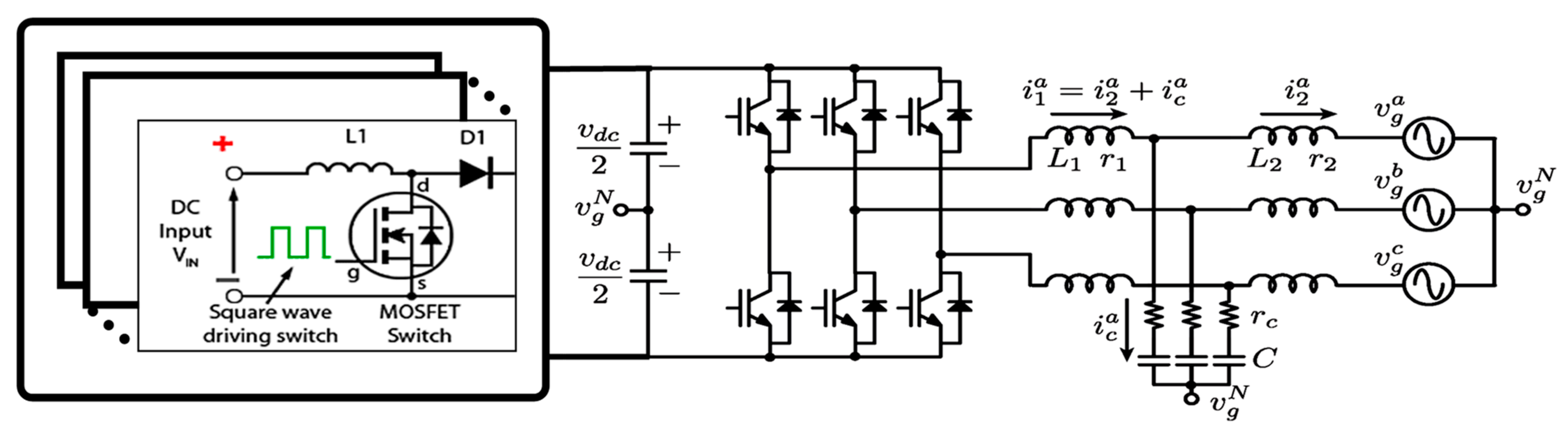
3.1. AC Filter
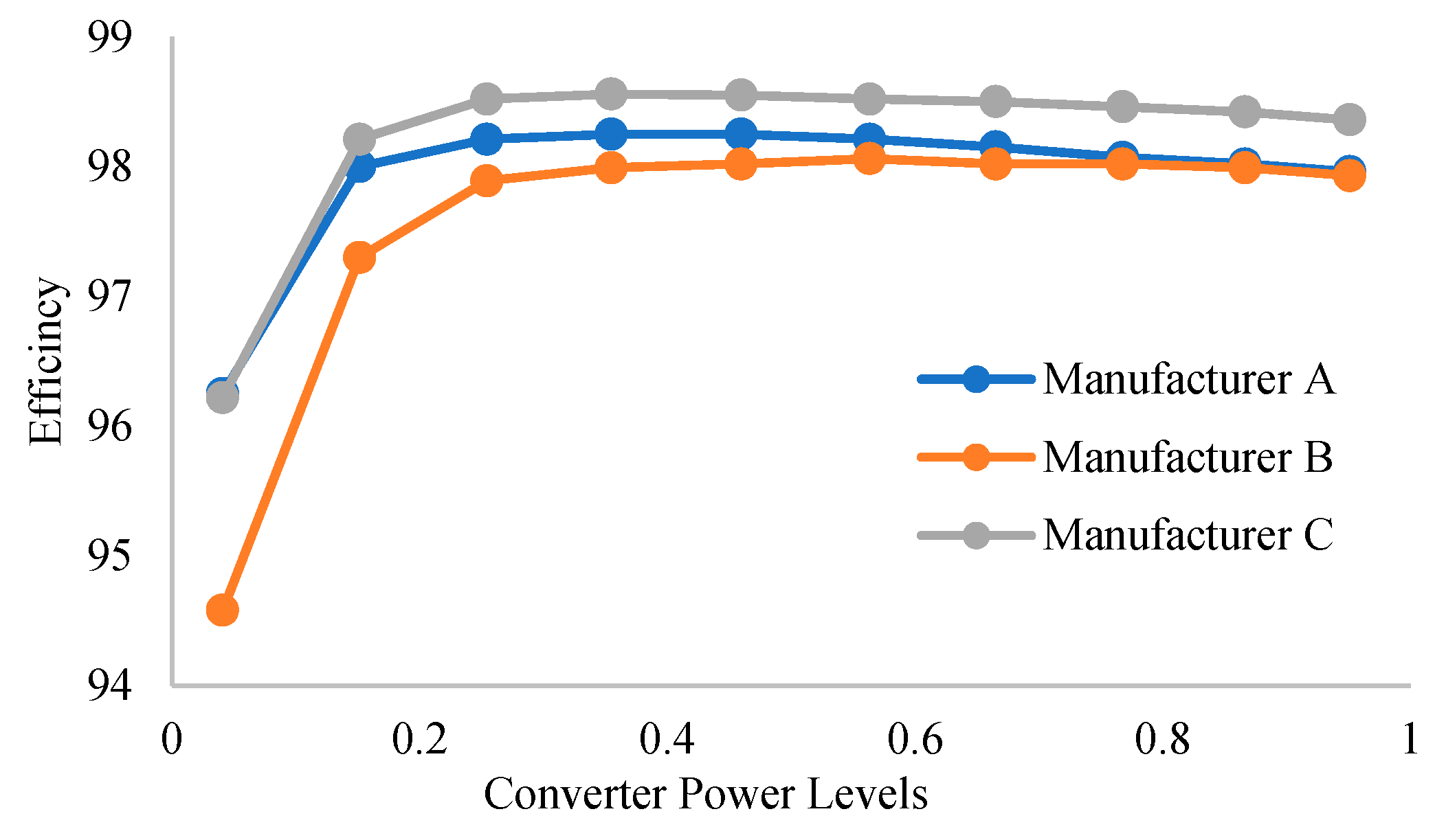
3.2. Inverter Losses
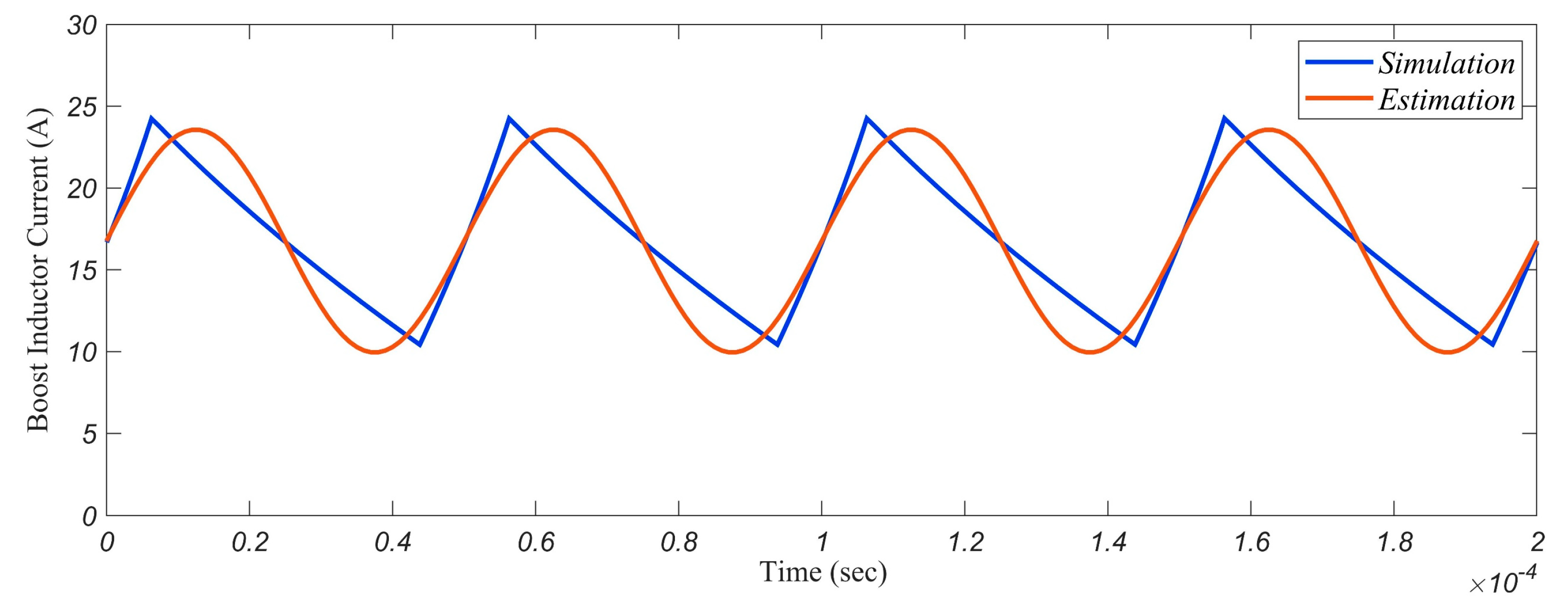
3.3. Boost Converter
3.4. DC-Link Capacitor
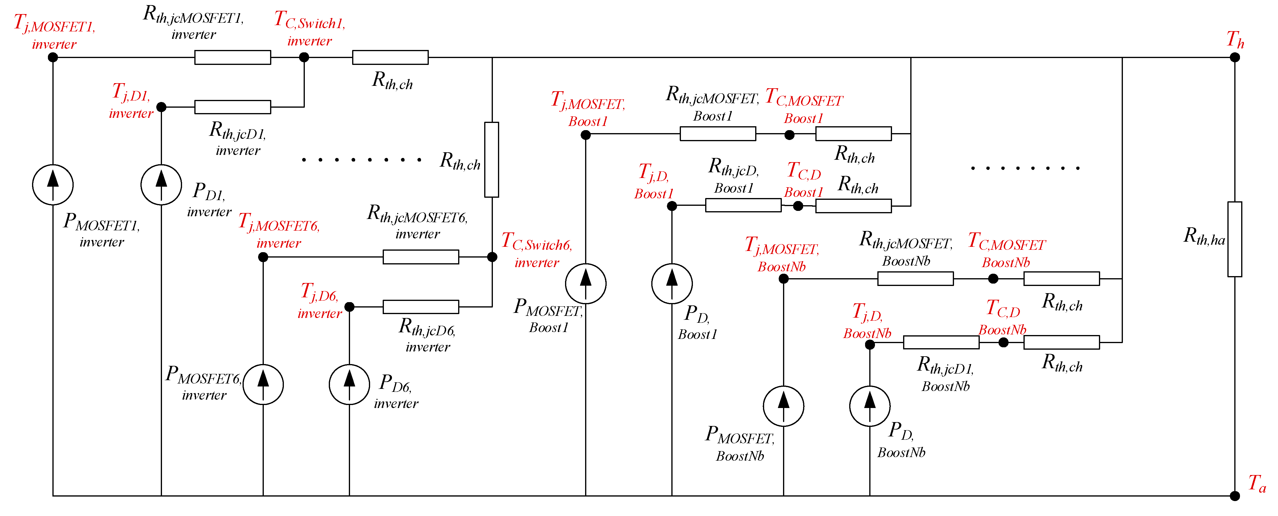
3.5. Thermal Model
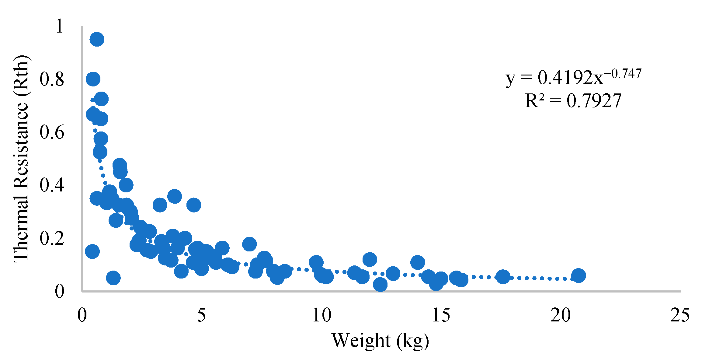
3.6. Heatsink Model
3.7. Reliability Model
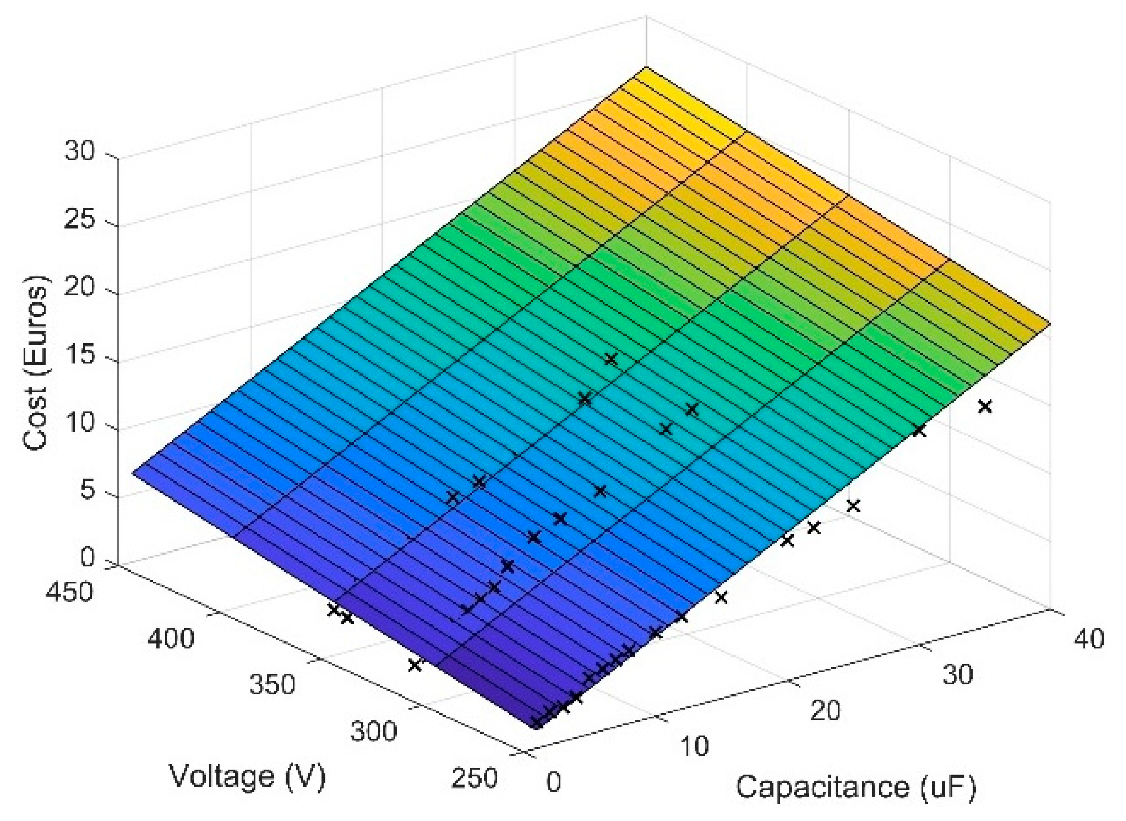
3.8. Cost Model
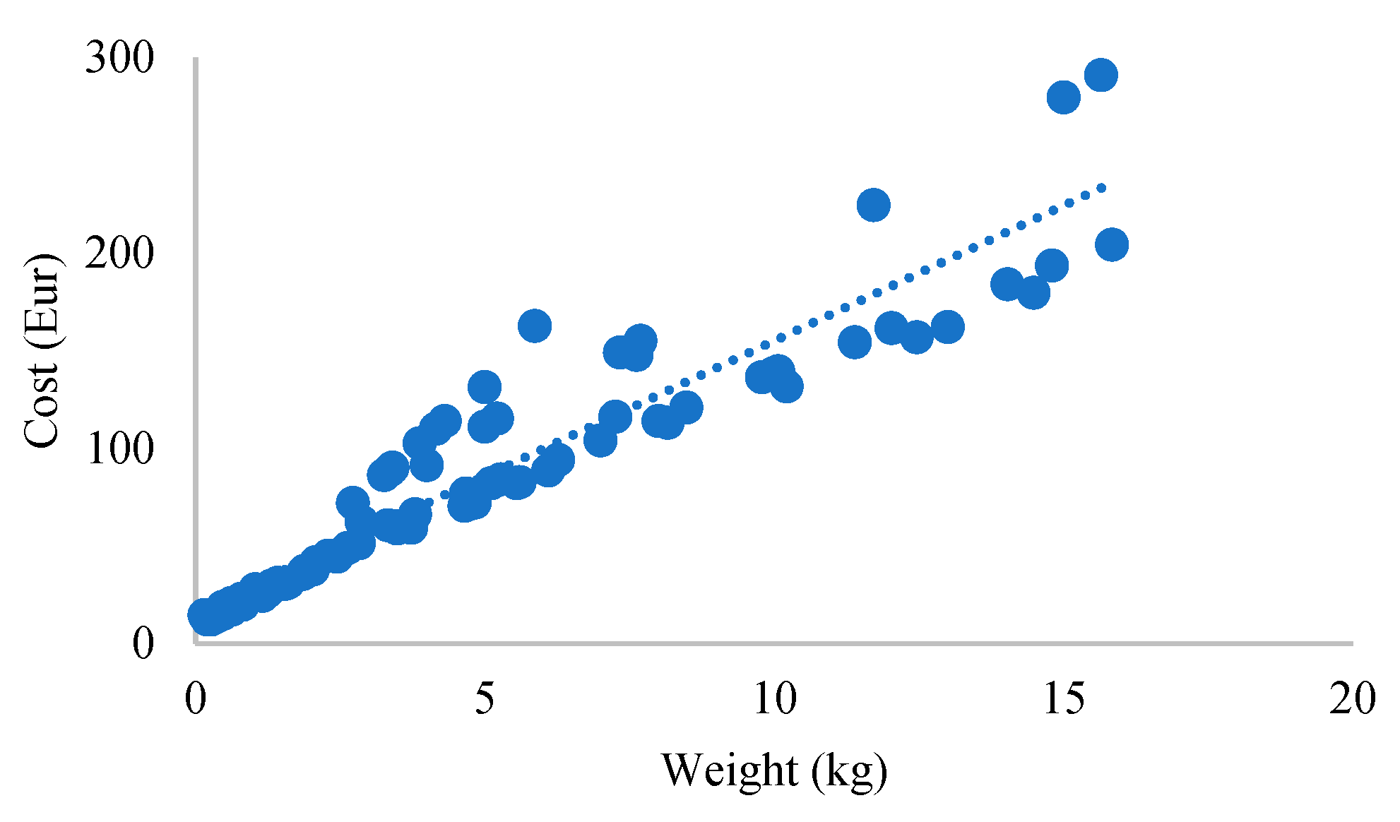
3.8.1. Semiconductor
3.8.2. Capacitors
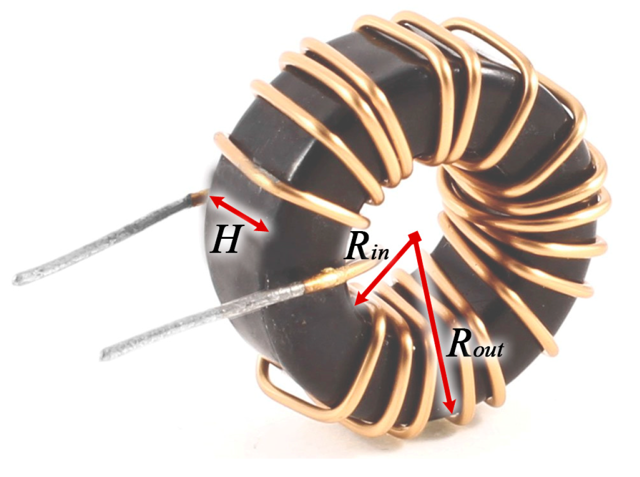
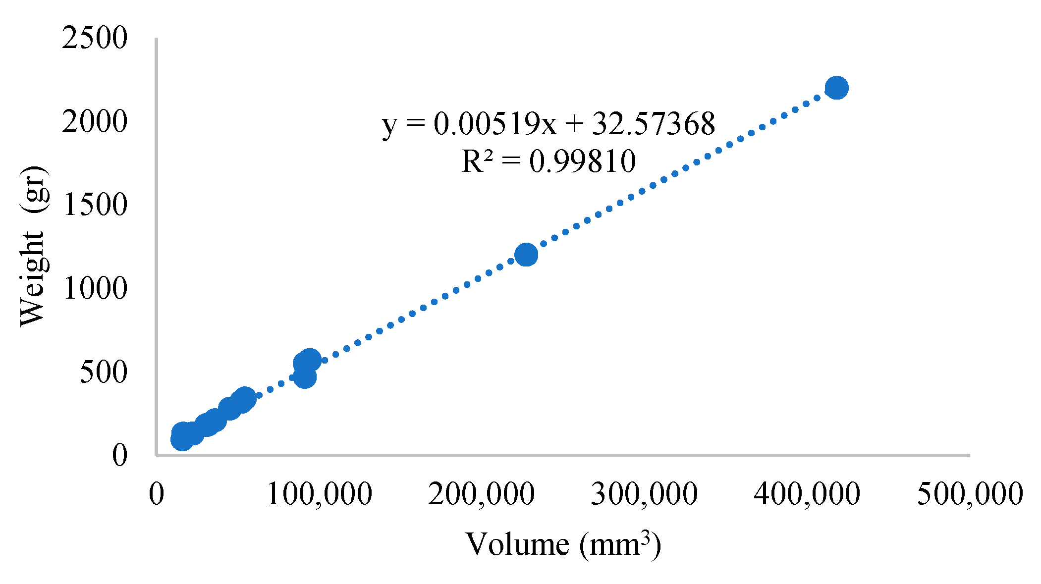
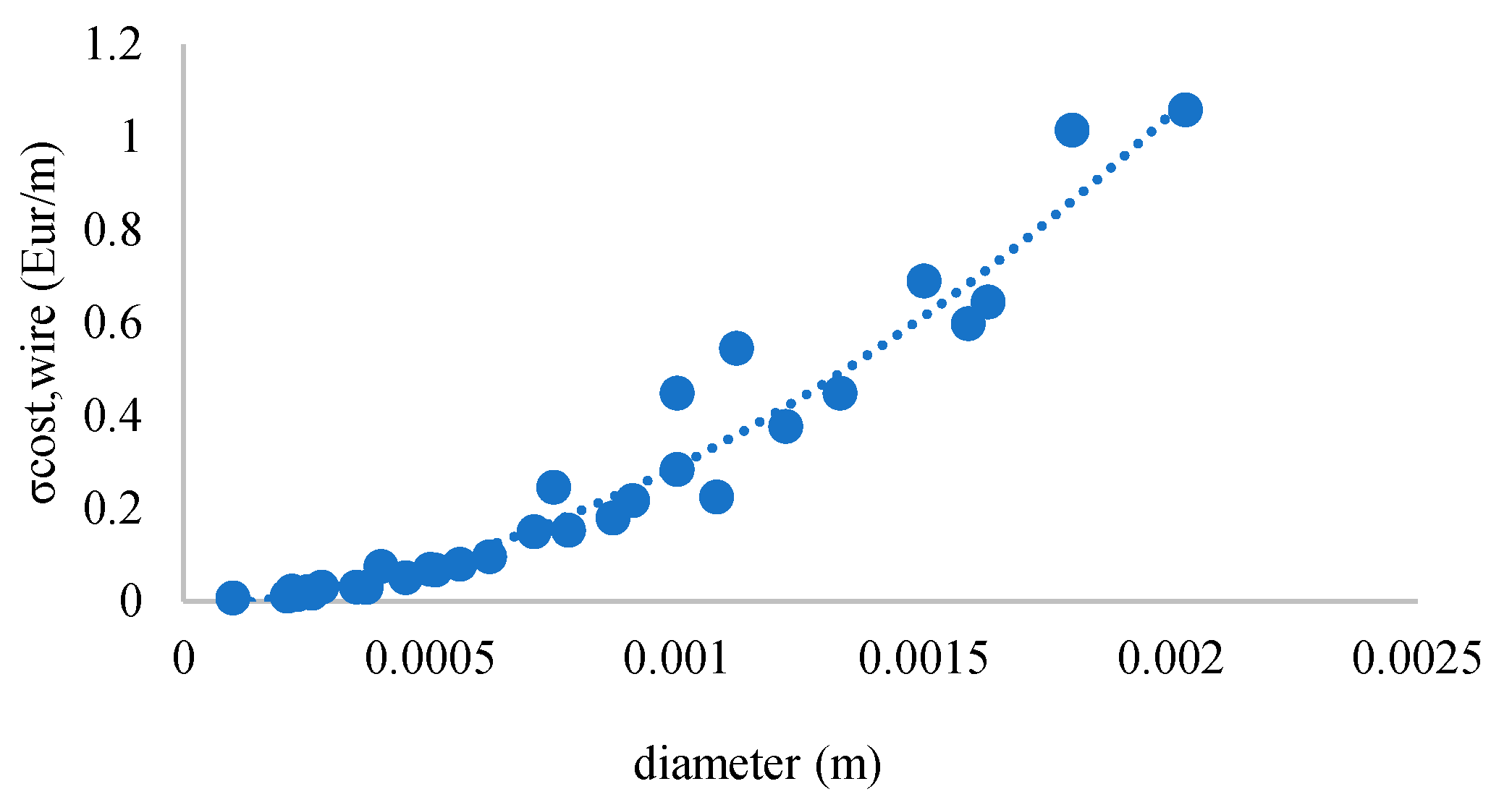
3.8.3. Inductors
3.8.4. Heatsink
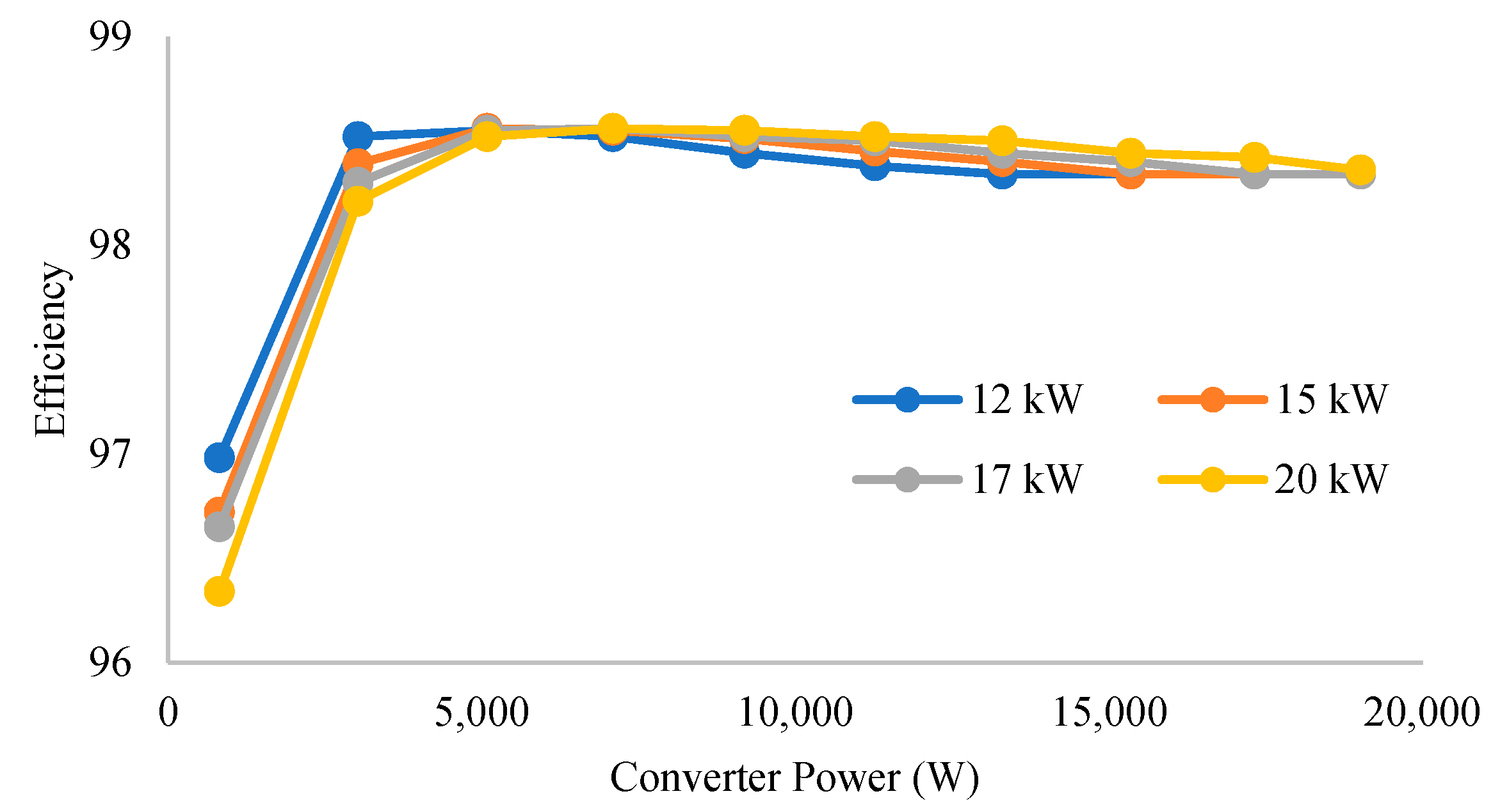
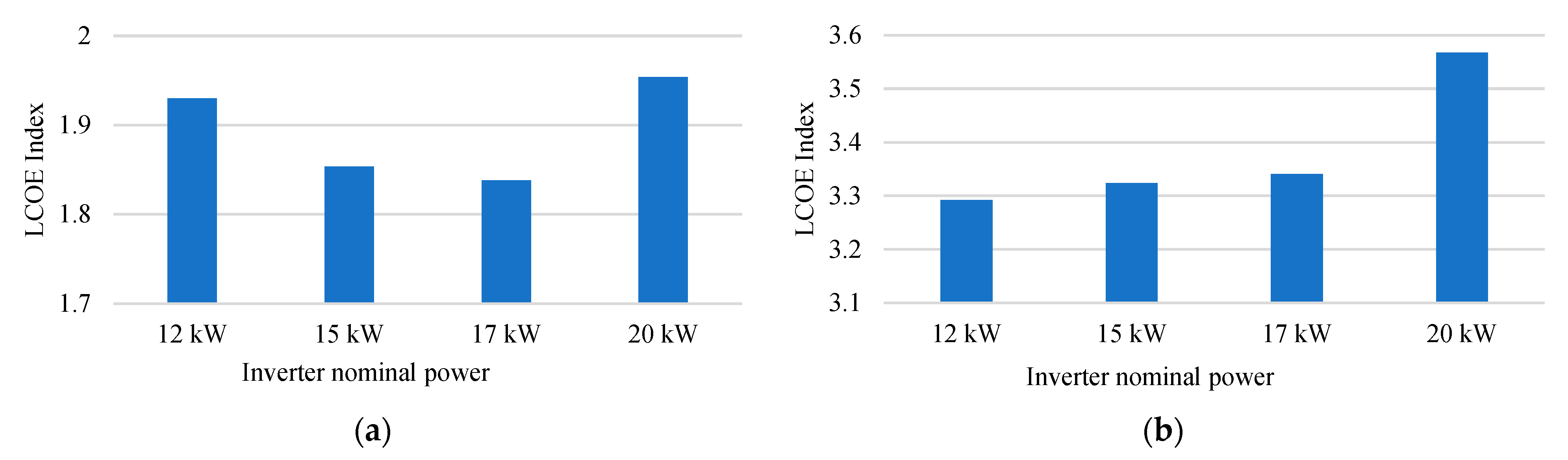
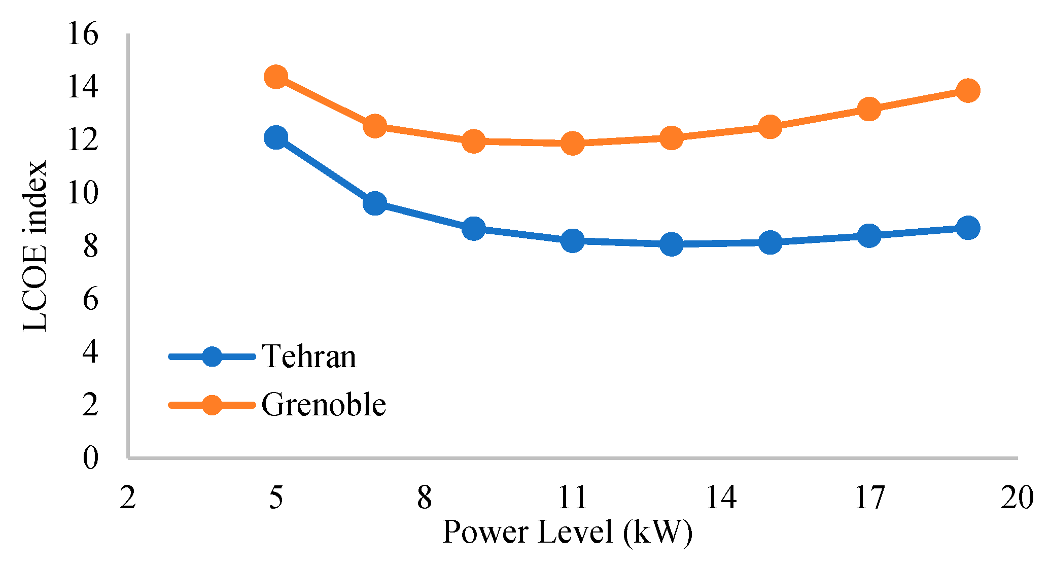
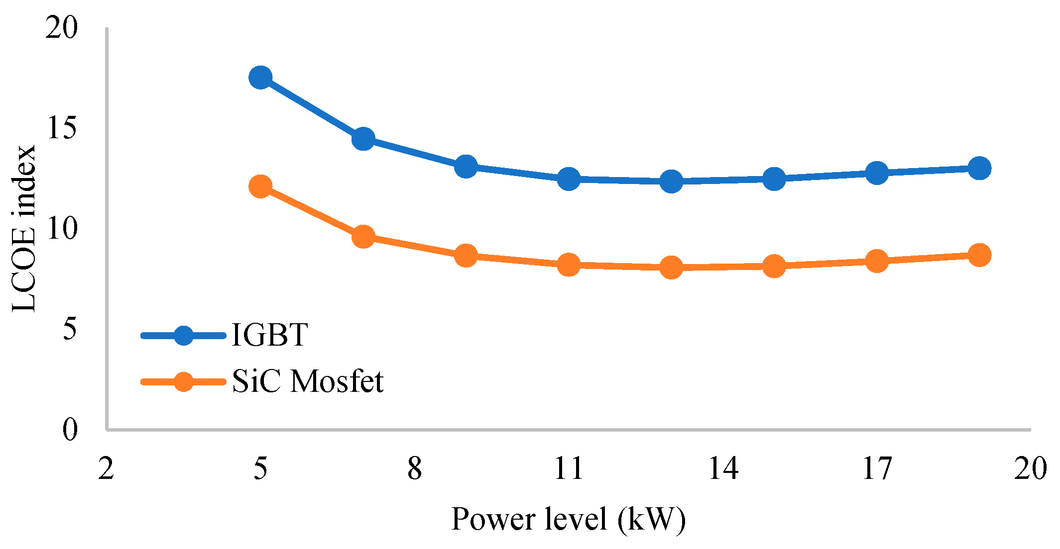
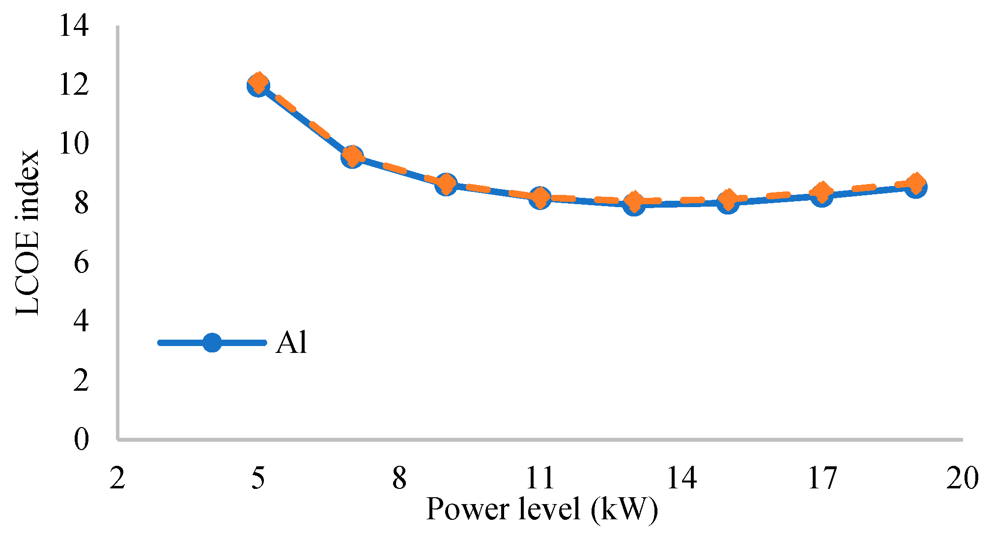
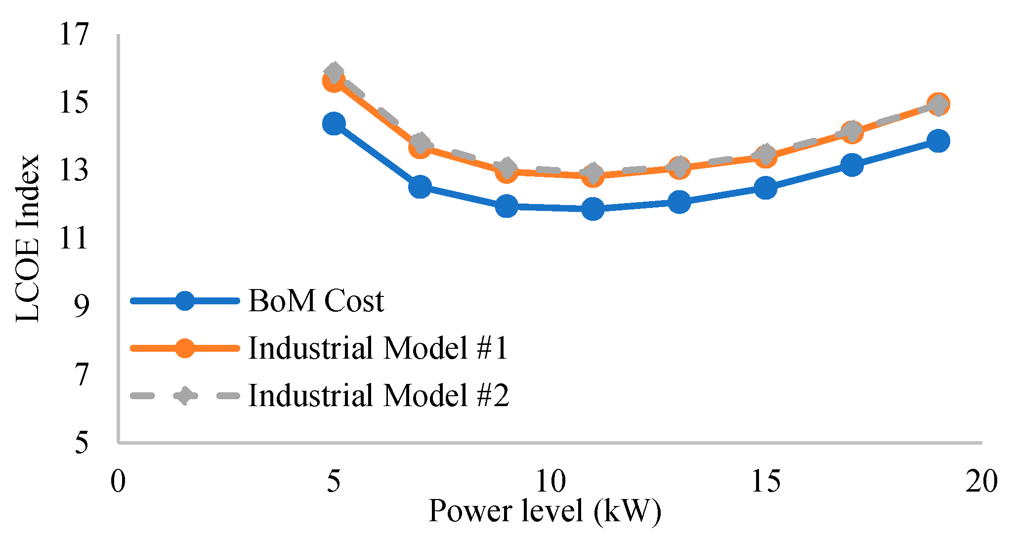
4. LCOE Estimation for Various Case Studies
5. Conclusions
Author Contributions
Funding
Data Availability Statement
Conflicts of Interest
References
- Feldman, D.; Ramasamy, V.; Fu, R.; Ramdas, A.; Desai, J.; Margolis, R.U.S. Solar Photovoltaic System Cost Benchmark: Q1 2020; NREL/TP-6A20-77324; National Renewable Energy Laboratory: Golden, CO, USA, 2021.
- Keller, L.; Affolter, P. Optimizing the panel area of a photovoltaic system in relation to the static inverter—Practical results. Sol. Energy 1995, 55, 1–7. [Google Scholar] [CrossRef]
- Koutroulis, E.; Blaabjerg, F. Design Optimization of Transformerless Grid-Connected PV Inverters Including Reliability. IEEE Trans. Power Electron. 2012, 28, 325–335. [Google Scholar] [CrossRef] [Green Version]
- Sangwongwanich, A.; Yang, Y.; Sera, D.; Blaabjerg, F. Mission Profile-Oriented Control for Reliability and Lifetime of Photovoltaic Inverters. In Proceedings of the 2018 International Power Electronics Conference (IPEC-Niigata 2018-ECCE Asia), Niigata, Japan, 20–24 May 2018; pp. 2512–2518. [Google Scholar] [CrossRef] [Green Version]
- Kadri, R.; Gaubert, J.-P.; Champenois, G. An Improved Maximum Power Point Tracking for Photovoltaic Grid-Connected Inverter Based on Voltage-Oriented Control. IEEE Trans. Ind. Electron. 2010, 58, 66–75. [Google Scholar] [CrossRef]
- Nasiri, R.; Khayamy, M.; Rashidi, M.; Nasiri, A.; Bhavaraju, V. Optimal Solar PV Sizing for Inverters Based on Specific Local Climate. In Proceedings of the 2018 IEEE Energy Conversion Congress and Exposition (ECCE), Portland, OR, USA, 23–27 September 2018; pp. 6214–6219. [Google Scholar] [CrossRef]
- Velasco, G.; Guinjoan, F.; Pique, R.; Conesa, A.; Negroni, J. Inverter power sizing considerations in grid-connected PV systems. In Proceedings of the 2007 European Conference on Power Electronics and Applications, Aalborg, Denmark, 2–5 September 2007; pp. 1–10. [Google Scholar] [CrossRef]
- Kratzenberg, M.G.; Deschamps, E.M.; Nascimento, L.; Rüther, R.; Zürn, H.H. Optimal Photovoltaic Inverter Sizing Considering Different Climate Conditions and Energy Prices. Energy Proc. 2014, 57, 226–234. [Google Scholar] [CrossRef] [Green Version]
- Solar, S.M.A.; Ag, T. INTEGRATED Service for Ease and Comfort. Available online: https://files.sma.de/downloads/STP15-25TL-30-DS-en-41.pdf (accessed on 23 April 2021).
- Fronius. Fronius Symo Datasheet. Available online: http://www.fronius.com/ (accessed on 22 September 2020).
- Huawei. Smart String Inverter. SUN2000-12/15/17/20KTL-M0 Datasheet, 2019. Available online: https://solar.huawei.com/-/media/Solar/attachment/pdf/apac/datasheet/SUN2000-12-20KTL-M0.pdf (accessed on 22 October 2020).
- De Leon-Aldaco, S.E.; Calleja, H.; Alquicira, J.A. Reliability and Mission Profiles of Photovoltaic Systems: A FIDES Approach. IEEE Trans. Power Electron. 2014, 30, 2578–2586. [Google Scholar] [CrossRef]
- Solar inverters. Solar Inverter for PV System|Europe Solar Store. Available online: https://www.europe-solarstore.com/solar-inverters.html?inverter_power=24 (accessed on 22 October 2020).
- Sangwongwanich, A.; Yang, Y.; Sera, D.; Blaabjerg, F. Lifetime Evaluation of Grid-Connected PV Inverters Considering Panel Degradation Rates and Installation Sites. IEEE Trans. Power Electron. 2017, 33, 1225–1236. [Google Scholar] [CrossRef] [Green Version]
- Orłowska-Kowalska, T.; Blaabjerg, F.; Rodríguez, J. Advanced and Intelligent Control in Power Electronics and Drives; Springer: Cham, Switzerland, 2014; Volume 531. [Google Scholar]
- Voldoire, A.; Schanen, J.; Ferrieux, J.; Gautier, C.; Saber, C. Optimal Design of an AC Filtering Inductor for a 3-Phase PWM Inverter Including Saturation Effect. In Proceedings of the 2019 10th International Power Electronics, Drive Systems and Technologies Conference (PEDSTC), Shiraz, Iran, 12–14 February 2019; pp. 595–599. [Google Scholar] [CrossRef]
- Voldoire, A.; Schanen, J.-L.; Ferrieux, J.-P.; Gautier, C.; Saber, C. Analytical Calculation of DC-Link Current for N-Interleaved 3-Phase PWM Inverters Considering AC Current Ripple. In Proceedings of the 2019 21st European Conference on Power Electronics and Applications, Genova, Italy, 3–5 September 2019. [Google Scholar] [CrossRef]
- Ahmed, M.H.; Wang, M.; Hassan, M.A.S.; Ullah, I. Power Loss Model and Efficiency Analysis of Three-Phase Inverter Based on SiC MOSFETs for PV Applications. IEEE Access 2019, 7, 75768–75781. [Google Scholar] [CrossRef]
- Kolar, J.; Round, S. Analytical calculation of the RMS current stress on the DC-link capacitor of voltage-PWM converter systems. IEE Proc.-Electr. Power Appl. 2006, 153, 535–543. [Google Scholar] [CrossRef] [Green Version]
- Shen, Y.; Song, S.; Wang, H.; Blaabjerg, F. Cost-Volume-Reliability Pareto Optimization of a Photovoltaic Microinverter. In Proceedings of the 2019 IEEE Applied Power Electronics Conference and Exposition (APEC), Anaheim, CA, USA, 17–21 March 2019; pp. 139–146. [Google Scholar] [CrossRef]
- Wakefield Thermal Air Cooled Thermal Extrusions. Available online: https://wakefieldthermal.com/thermal-solutions/air-cooled/thermal-extrusions/ (accessed on 26 February 2019).
- FIDES Guide 2009. Edition A. Reliability Methodology for Electronic Systems. 2010. Available online: www.fides-reliability.org (accessed on 29 September 2010).
- Burkart, R.; Kolar, J.W. Component cost models for multi-objective optimizations of switched-mode power converters. In Proceedings of the 2013 IEEE Energy Conversion Congress and Exposition, Denver, CO, USA, 15–19 September 2013; pp. 2139–2146. [Google Scholar] [CrossRef]
- Capacitors Datasheet, Vishay. Available online: https://www.vishay.com/en/capacitors/ (accessed on 15 June 2020).
- Capacitors Datasheet, TDK. Available online: https://product.tdk.com/en/products/capacitor/index.html (accessed on 10 September 2019).
- Powder Cores Datasheets, Magnetics. Available online: https://www.mag-inc.com/Products/Powder-Cores (accessed on 17 August 2017).
- Voldoire, A. Outil de Développement et D’optimisation Dédié aux Onduleurs SiC de Forte Puissance. Doctoral Dissertation, Université Grenoble Alpes, Saint-Martin-d'Hères, France, 2020. [Google Scholar]
- Energy Chains, Polymer Bearings, Flexible Cable & Linear Slides. Available online: https://www.igus.co.uk/ (accessed on 15 June 2020).
- Wakefield-Vette Heat Sinks–Mouser Europe. Available online: https://eu.mouser.com/c/thermal-management/heat-sinks/?m=Wakefield-Vette (accessed on 15 June 2020).
- Boggs, P.T.; Tolle, J.W. Sequential Quadratic Programming. Acta Numer. 1995, 4, 1–51. [Google Scholar] [CrossRef] [Green Version]
- Giancoli, D.C. Physics, 4th ed.; Prentice Hall: Hoboken, NJ, USA, 1995. [Google Scholar]


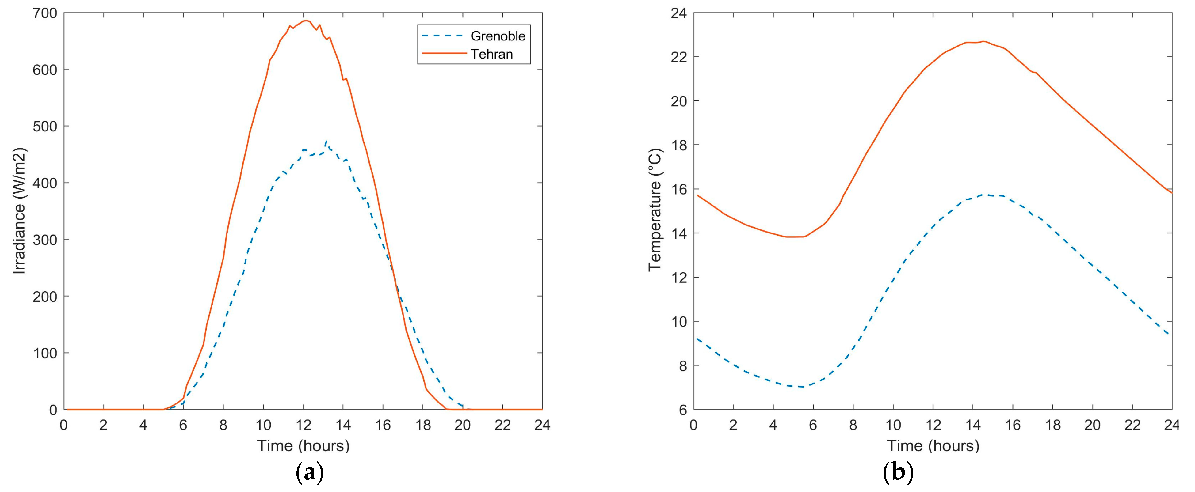
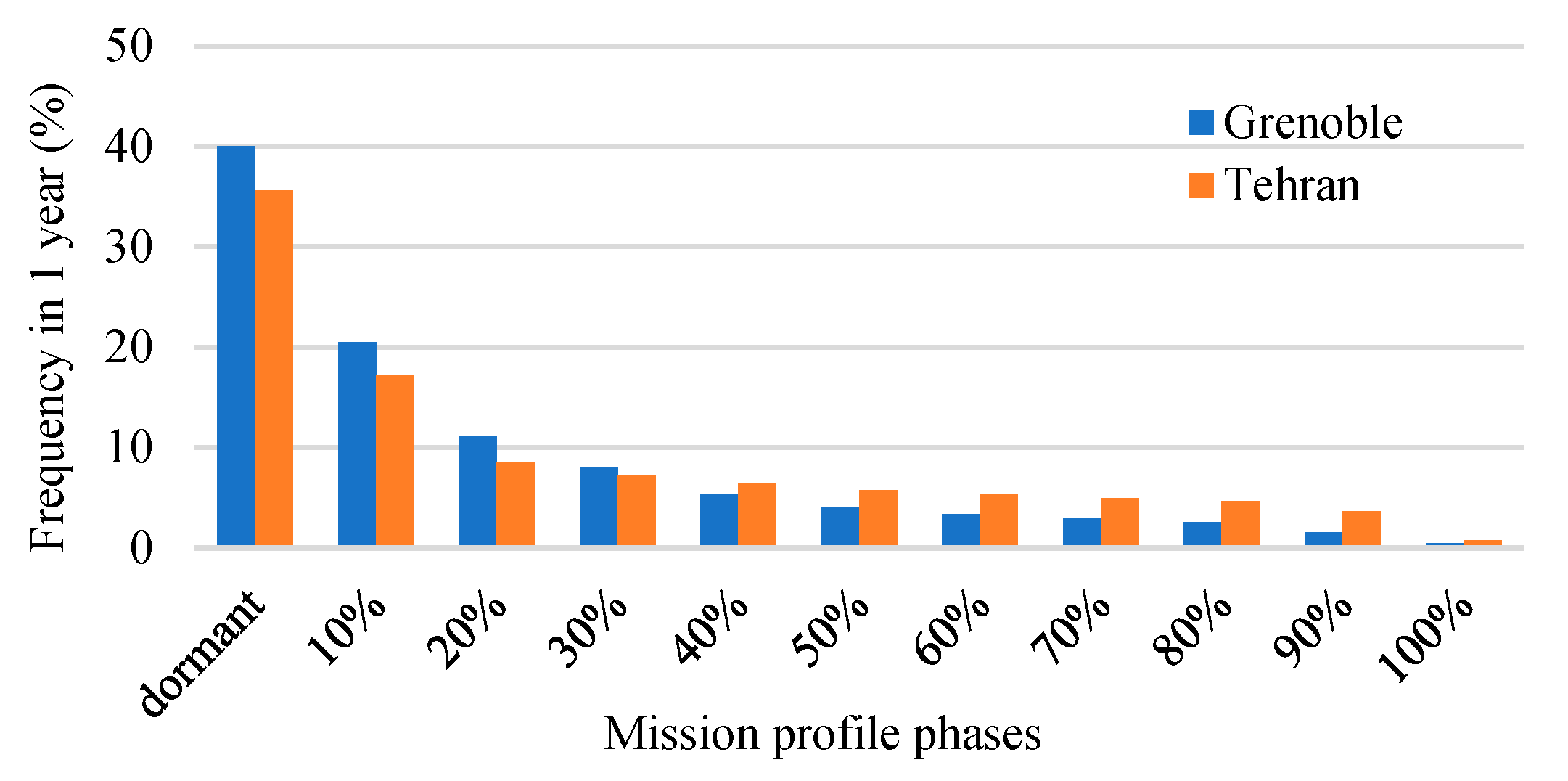
| Phase | Grenoble | Tehran | |||||||
|---|---|---|---|---|---|---|---|---|---|
| hL (Hour) | TL (°C) | Vpv (V) | Ppv (W) | hL (Hour) | TL (°C) | Vpv (V) | Ppv (W) | ||
| Pmax = 20.533 kW | dormant | 3504 | 10.4 | 0 | 0 | 3116 | 16 | 0 | 0 |
| 10% | 1796 | 11.5 | 610 | 823 | 1500 | 17 | 590 | 741 | |
| 20% | 975 | 13.4 | 639 | 3032 | 743 | 18.1 | 628 | 2974 | |
| 30% | 708 | 15.3 | 641 | 5089 | 637 | 19 | 634 | 4985 | |
| 40% | 468 | 17.1 | 638 | 7096 | 562 | 20.4 | 634 | 6997 | |
| 50% | 360 | 18.7 | 633 | 9195 | 501 | 22.2 | 629 | 8998 | |
| 60% | 295 | 19.8 | 629 | 11,270 | 474 | 24.3 | 624 | 11,001 | |
| 70% | 254 | 20.9 | 623 | 13,305 | 435 | 26.6 | 612 | 13,004 | |
| 80% | 223 | 21.7 | 618 | 15,351 | 410 | 28.4 | 604 | 14,994 | |
| 90% | 137 | 22 | 613 | 17,328 | 318 | 29.5 | 597 | 16,970 | |
| 100% | 40 | 22.1 | 611 | 19,017 | 65 | 30.1 | 594 | 18,478 | |
Disclaimer/Publisher’s Note: The statements, opinions and data contained in all publications are solely those of the individual author(s) and contributor(s) and not of MDPI and/or the editor(s). MDPI and/or the editor(s) disclaim responsibility for any injury to people or property resulting from any ideas, methods, instructions or products referred to in the content. |
© 2023 by the authors. Licensee MDPI, Basel, Switzerland. This article is an open access article distributed under the terms and conditions of the Creative Commons Attribution (CC BY) license (https://creativecommons.org/licenses/by/4.0/).
Share and Cite
Tadbiri-Nooshabadi, M.; Schanen, J.-L.; Farhangi, S.; Iman-Eini, H.; Rizet, C. Optimal Design of PV Inverter Using LCOE Index. Energies 2023, 16, 2213. https://doi.org/10.3390/en16052213
Tadbiri-Nooshabadi M, Schanen J-L, Farhangi S, Iman-Eini H, Rizet C. Optimal Design of PV Inverter Using LCOE Index. Energies. 2023; 16(5):2213. https://doi.org/10.3390/en16052213
Chicago/Turabian StyleTadbiri-Nooshabadi, Morteza, Jean-Luc Schanen, Shahrokh Farhangi, Hossein Iman-Eini, and Corentin Rizet. 2023. "Optimal Design of PV Inverter Using LCOE Index" Energies 16, no. 5: 2213. https://doi.org/10.3390/en16052213