Modelling the Operation Process of Light Utility Vehicles in Transport Systems Using Monte Carlo Simulation and Semi-Markov Approach

Abstract

This research paper presents studies on the operation process of the Honker 2000 light utility vehicles that are part of the Polish Armed Forces transport system. The phase space of the process was identified based on the assumption that at any given moment the vehicle remains in one of four states, namely, task execution, awaiting a transport task, periodic maintenance, or repair. Vehicle functional readiness and technical suitability indices were adopted as performance measures for the technical system. A simulation model based on Monte Carlo methods was developed to determine the changes in the operational states. The occurrence of the periodic maintenance state is strictly determined by a planned and preventive strategy of operation applied within the analysed system. Other states are implementations of stochastic processes. The original source code was developed in the MATLAB environment to implement the model. Based on estimated probabilistic characteristics, the authors validated 16 simulation models resulting from all possible cumulative distribution functions (CDFs) that satisfied the condition of a proper match to empirical data. Based on the simulated operation process for a sample of 19 vehicles over the assumed 20-year forecast horizon, it was possible to determine the functional readiness and technical suitability indices. The relative differences between the results of all simulation models and the results obtained through the semi-Markov model did not exceed 6%. The best-fit model was subjected to sensitivity analysis in terms of the dependence between functional readiness and technical suitability indices on vehicle operation intensity. As a result, the proposed simulation system based on Monte Carlo methods turned out to be a useful tool in analysing the current operation process of means of transport in terms of forecasts related to a current environment, as well as when attempting its extrapolation.

1. Introduction

Simulation models based on Monte Carlo methods involve repeated performances of a certain random experiment. Initially, they were used to numerically determine the number value of π, calculate the integrals of complex functions as the area under the graph, and determine the probability of random events [1,2]. Developing an algorithm that depicts the course of changes in complex processes and implementing it within software enables the solution of a complex analytical problem using simulation methods [3,4,5,6,7].

Markov models [8,9] and semi-Markov models [10,11] are often used to analyse and evaluate the operation processes. They require a thorough analysis of the stochastic process through the identification of possible states and the description of probabilistic characteristics for interstate transition times. The elements of the transition intensity matrix for Markov models are identified as reciprocals of the expected times of transition between individual states. However, in the case of mechanical vehicles, the probabilistic characteristics determined within a time domain describe the intensity of the operation sub-process in a rather vague manner. The value of the vehicle with technical service life exhaustion is a reflected unit of measure of the work performed, expressed by the covered mileage (distance). Furthermore, probabilistic characteristics that describe the correct operating intervals of the vehicle between successive failures can be expressed within the mileage domain [12,13].

This study is a continuation of the research in the field of reliability and readiness of light utility vehicles. Previous publications in this field focused on analysing reliability based on censored failure damage [12] and modelling readiness through the application of Markov theory [14] and semi-Markov process theory [15]. After analysing a true operation’s process, the authors developed a four-state simulation model employing Monte Carlo methods. It was assumed that the operation of light utility vehicles is a mixed process, that is, random-deterministic. Consequently, operation plans reflect the deterministic nature, which is, however, interrupted by random events of a stochastic character [6]. This result is from the planned and preventive technical maintenance strategy applied within the operating system of the studied vehicle population. The proposed innovative simulation model was verified based on determined probabilistic characteristics of individual operation, maintenance, and overhaul sub-processes. The model’s undoubted advantage is its held ability to determine the values of functional readiness and technical suitability indices not only relative to current operating conditions but also to enable forecasting of their values in the case of hypothetically possible scenarios.

The approach to modelling an operation process presented in this paper supplements the current state of knowledge, which is discussed in the form of a source literature review. The iterative algorithm developed for the model based on Monte Carlo methods enables simulating a process composed of both stochastic and deterministic sub-processes. The achievement of particular operating states by vehicles in a transport system is carried out according to probabilistic characteristics. The cumulative distribution functions of daily mileage, repair time, and reliability function determine the course of the realisation of stochastic processes in the system. Periodic maintenance is a process strictly determined by the operating strategy. The numerical analyses carried out that make up part of this study refer to the operation of a selected population of light utility vehicles; however, the proposed model can also be applied to the analysis of other technical objects after appropriate modifications. It should also be stressed that the presented approach to simulation modelling, as well as the analysis of other technical objects, has not previously been the subject of research by other authors. The iterative algorithm developed is designed both to assess the efficiency of the operation of the transport system under current conditions and to forecast its performance under hypothetical conditions.

Additionally, the choice of the Honker 2000 as the subject of this study is justified by the significant importance of light utility vehicles in military transport systems. Assessment and prediction of the readiness and suitability of these technical objects are necessary for the planning of training and combat operations. In the reality of constant change and the emergence of new challenges, the proposed iterative Monte Carlo algorithm and the four-state operation model are valuable tools in engineering and military practise. The superiority of the proposed simulation approach over Markov and semi-Markov models is the extrapolation of the model over a wide range of variability in the intensity of the operation processes.

The purpose of this work is to develop a simulation model for the analysis, evaluation, and prediction of the efficiency and reliability of vehicle operating processes in transport systems. The main contributions of this paper are as follows:

• Development of a simulation model based on Monte Carlo methods;
• Implementation of the Monte Carlo model in the MATLAB environment;
• Validation of simulation models based on the analytical approach of a four-state semi-Markov process;
• Evaluation of the operation and maintenance processes of light utility vehicles using the proposed indicators and sensitivity analysis resulting from changes in the intensity parameters of the operational process.

This paper is divided into six sections. The literature review covers the current state of knowledge and shows the research published by other authors. In section three, several assumptions are made, and the simulation model based on Monte Carlo methods is presented with estimations of the probabilistic characteristics of sub-processes that determine whether a vehicle remains in individual operating states. The semi-Markov approach was developed in section four. Section five presents the results of the simulations and stochastic models. The Monte Carlo and semi-Markov models had almost the same functional readiness and technical suitability indicators, which is why the sensitivity analysis was developed for the above-mentioned models. In the end, the research is summarised and our final conclusions are formulated.

2. Literature Review

Several research papers employ Monte Carlo models for reliability studies [16,17,18,19,20]. Zhang et al. [21] used the Monte Carlo simulation to estimate the optimal parameters of a fault location model for wind turbines. Kallen [22] suggested a simulation model for a renewable object repair process with characteristics consistent with the exponential and Weibull distributions. Durczak et al. [23] used Monte Carlo techniques, Latin hypercube sampling, and Iman–Conover methods to generate time-to-failure data from the Weibull distribution. In contrast, the application of simulations within reliability studies of computer networks by Benson and Kellner [1] enables estimating the mean time-to-failure in an easier manner than with traditional methods. Simulation and computational methods relative to power supply systems are compared in [24]. In the case of both methods, the waveforms of the reliability function are very similar. Studies on the reliability of boat positioning systems involve developing a Monte Carlo model based on the probabilistic characteristics of its individual components [25]. A similar approach is presented in relation to photovoltaic systems when determining the reliability function for the entire system [26]. Green et al. [27] developed a complex simulation algorithm based on the Monte Carlo method and intelligent state space pruning (ISSP) combined with genetic algorithms (GA), particle swarm optimisation (PSO), ant colony optimisation (ACO), and artificial immune system optimisation (AIS). This solution reduced computational time by 50-90% compared to the non-sequential Monte Carlo simulation in the reliability analysis of electrical power systems.

Roslan et al. [28] developed a two-state reliability model, which was then verified through sequential and non-sequential simulations. In terms of reliability index estimation accuracy, the sequential Monte Carlo model turned out to be more effective than the non-sequential version. Research on the technical readiness of rotary drilling machines as renewable objects involved developing a simulation model based on Monte Carlo methods and Markov chain theory [29]. Here, the parameters of the reliability function were estimated based on times between failures. In their paper, for each 10 h period, it was determined with an 80% probability that a system composed of ten drilling machines will have five to eight such objects ready for operation. Whereas in [30], Monte Carlo sequential algorithms were used to determine the remaining useful life. The Monte Carlo Markov chain simulation algorithm [31] was developed to optimise maintenance policy and resulted in a 10% reduction in total costs for every mile of track.

Zhang et al. [32] proposed a method combining Monte Carlo simulations and directional sampling to analyse object reliability sensitivity. This method is based on the nearest Euclidean distance strategy. The accuracy and effectiveness of the proposed method were proved through practical numerical examples. In turn, Zhang et al. [33] evaluated the reliability of a power station by adopting a four- and five-state reliability model. They demonstrate that an approach based on the sequential Monte Carlo method is more rigorous than classical methods and that the calculated reliability indices adopt lower values. A novel method for evaluating the reliability of renewable objects is proposed in [5]; the authors combined Monte Carlo methods with fault trees. In relation to the field of readiness and reliability of military structures, the authors of [34] conducted Monte Carlo simulations for three strategies for managing the platform operation processes, namely, replacing as needed, re-inspection at a specified interval, and prognostics. The prognostic approach optimised the operational readiness of military equipment by forecasting damage and reducing logistics delays. In addition, determining the remaining functional period of structures supports commanders in selecting appropriate platforms to implement future missions, resulting in a reduced failure risk.

The issues related to the simulation modelling of transport systems are presented in [35]. The authors analysed mass transit that provides transport services on 20 routes. The performance characteristics of individual drivers and vehicle reliability were used to optimise transport processes. Performing 10,000 simulation steps enable one to estimate the expected number of unrealized trips and the level of reduction in operating costs within a transport system, depending on the availability and reliability of the driver. The same number of simulations were conducted in the case of the Markov Chain Monte Carlo (MCMC) in [36], developed for a four-state phase space of the electrical vehicle operation process. In another paper [37], a Monte Carlo simulation based on the probability distribution function of the travel time was used to estimate the expected secondary delays of the trips. In

Table 1. Review of literature on the Monte Carlo approach for reliability and availability analysis.

Methods	Purposes of Research	Case Studies	Simulations	Papers
Monte Carlo	Reliability analysis	Coated surface	Sampling of inter-repair time (500 samples)	[22]
Monte Carlo, Latin hypercube sampling (LHS) and Iman-Conover methods	Reliability analysis	Agricultural tractors	Sampling of time-to-failure data	[23]
Markov Chain Monte Carlo	Reliability and availability analysis	Rotary drilling machines	Simulation of Markov Chain transitions	[29]
Markov Chain Monte Carlo	Global minimization of the system failure probability	Structural dynamic systems under stochastic excitation: linear single-degree of freedom system, linear eight-story two dimensional frame structure and a nonlinear three dimensional bridge structural	Random sampling of many variables	[17]
Markov Chain Monte Carlo	Modelling of vehicle use patterns	Electric vehicles	Random sampling of daily driving time (105 trials)	[36]
Markov Chain Monte Carlo and Sequential Monte Carlo	Assessment of remaining useful life	Milling machine	Sampling from posteriori distribution of states	[30]
Markov Chain Monte Carlo with the Metropolis–Hasting Algorithm	Reliability assessment	Bridge health monitoring	Sampling of points to estimate failure probability	[18]
Sequential Markov Chain Monte Carlo	Optimisation of preventive maintenance schedule	Isolated Distributed Cuban Power System (wind turbines)	Simulation of wind speed	[38]
Sequential and Non-sequential Monte Carlo	Reliability assessment	Distribution network	Simulation by sampling of time-to-failure and time-to-repair	[28]
Monte Carlo and Copula	Power demand prediction	Electric vehicles	Simulation by sampling start time, end time, and distance travelled	[39]
Monte Carlo and directional sampling	Reliability sensitivity analysis	Headless rivet and wing box structure	Random sampling data (1 × 106 and 2 × 106)	[32]
Deep Belief Network and Monte Carlo	Calculate the reliability of the model	Physically-based thermal error model of the servo axis in machine tool	Random sampling data (107 trials) of the thermal characteristic parameters	[16]
Iterative Monte Carlo and semi-Markov approach	Assessing readiness and forecasting in various operational scenarios	Transportation system equipped with light utility vehicles	Sampling of task assignments, daily mileages, failures, and repairs based on CDFs and reliability function	This paper

, some selected works on the application of the Monte Carlo approach to reliability and readiness research for a spectrum of technical facilities and systems are summarised.

Unlike previous studies, this publication presents a simulation model that takes into account random-deterministic processes. In the process of vehicle operation, periodic maintenance was adopted according to the documentation, taking into account time intervals or the amount of work performed in order to reliably reflect the phase trajectory for the vehicle. A novelty in this publication is the development of a four-state model adapted to the specificity of the Honker 2000 light utility vehicles, in accordance with the adopted modelling goal. Furthermore, the intention of the authors was to check which research method would prove to be more effective. Our findings suggest that the Monte Carlo simulation model turned out to be a slightly better forecasting tool compared to the semi-Markov model.

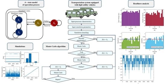
3. Monte Carlo Approach

All variables used for simulation modelling are listed in

Table 2. Notations and definitions.

Notations	Definitions
X(t)	Stochastic process
Tm	Normative period between maintenance
Lm	Normative mileage between maintenance
tm(t)	Time since last periodic maintenance
lm(t)	Mileage since last periodic maintenance
Θ	Probability of assignment task
κ	Redundancy
ld	Daily mileage
ldmax	Maximum daily mileage
lr	Mileage since last failure
lf	Mileage on the day of failure
G(ld)	Cumulative distribution function (CDF) of daily mileage
R(lr)	Reliability function
F(lr)	Cumulative distribution function (CDF) of failures
f(lr)	Probability density function (PDF) of failures
H(i)	Cumulative distribution function (CDF) of repair time
q1, q2, q3, q4	Random values of the uniform distribution on the interval (0, 1)
T(S1), T(S2), T(S3), T(S4)	Sojourn times of state S1, S2, S3, S4
Kr	Readiness indicator
Ks	Suitability indicator
Nv	Number of vehicles
Zi	Number of iterations

. A four-state vehicle operation process space was assumed for the proposed modelling method. The importance and description of individual states can be found in

Table 3. Operation process state space.

State	Meaning	Description
S1	Task execution	Vehicle is assigned to perform transportation tasks.
S2	Awaiting a transport task	Vehicle in reserve is waiting for a task.
S3	Periodic maintenance	Periodic maintenance is required. Vehicle is being serviced.
S4	Repair	Vehicle has failed. Repair is completed or vehicle is pending repair.

. Vehicle operation can be understood in this case as a process of changes in the operational states implemented within a calendar time. These changes are determined through operational strategy, operation processes, reliability of system components, and the organisation and efficiency of a technical system responsible for maintenance and operation. Due to the functional specificity of military transport systems (in the case of a defined state space), the authors adopted the assumption that on a given day, the vehicle is in exactly one operational state. The phase space of the process contains states that are significant from the perspectives of functional readiness and technical suitability. Compared to a nine-state model [15], the four-state model is simplified by eliminating short-term operational states, such as refuelling and maintenance performed both before and after the execution of the task. Furthermore, operational states that involve a vehicle staying in a technical unsuitability state, i.e., diagnosis (searching for damage causes) or awaiting repair or repair, are aggregated into a single state defined as ‘repair’.

Developing probabilistic characteristics is the basis for constructing a proposed simulation model based on Monte Carlo methods. The analysis was conducted through operational testing covering a sample of 19 Honker 2000 vehicles operated by the transport system of a military unit. These vehicles are intended to transport passengers and cargo weighing less than 1000 kg. They constitute a significant component of the transport capabilities of the Polish Armed Forces.

A three-element subset of technical suitability states, where an object is not damaged and does not require repair, was distinguished in the four-state operation model. This subset contains a two-element subset of functional readiness states, where the vehicle is ready or is performing transport tasks. Figure 1 is a graphical representation of the operational state distribution, together with vectors symbolising possible inter-state transitions.

On the basis of the simulation results, the efficiency of the operation processes is assessed on the basis of suitably selected indicators. For the four-state model, two indicators were proposed to describe vehicle readiness: availability and suitability. The readiness index K_r corresponds to the probability that a technical object is in a subset of readiness states, which for the four-state model refers to states S₁ and S₂. Technical suitability expresses the condition of an object in which it is not damaged and repair is not required [15]. The technical suitability index K_s is the probability that the vehicle is in a subset of technical suitability states, i.e., states S₁, S₂, and S₃. The values of these indices are calculated according to the following relationships:

$$K_r=\frac{T\left(S_1\right)+T\left(S_2\right)}{{\displaystyle \sum _{i=1}^{4}T\left(S_i\right)}},$$

(1)

$$K_s=\frac{T\left(S_1\right)+T\left(S_2\right)+T\left(S_3\right)}{{\displaystyle \sum _{i=1}^{4}T\left(S_i\right)}}.$$

(2)

3.1. Periodic Maintenance

Within the planned and preventive strategy for vehicle operation process management, periodic maintenance tasks are implemented at strictly specified time and mileage intervals. According to its assumptions, strictly defined maintenance tasks are performed after completing a specified amount of work, usually expressed in engine hours or kilometres [40,41]. However, it should be noted that all types of chemical, biological, and climatic factors acting on technical objects favour the physical ageing of assemblies, subassemblies, mechanisms and machinery components, as well as operating fluids [42,43]. This implies the need to define maximum intervals between successive maintenance tasks, usually expressed in months or years [44,45,46,47,48].

Such an organisation of vehicle maintenance circumscribes the deterministic nature of implementing this sub-process. A mathematical description of an event involving process X(t) reaching state S₃ is expressed by the following relationship:

$$\left(t_m\left(t\right)\ge T_m\vee l_m\left(t\right)\ge L_m\right)\Rightarrow X\left(t\right)=S_3.$$

(3)

The incidence of state S₃ is mainly affected by the intensity of the operation process, which is determined by the probability of assigning a transport task to a vehicle and the daily mileage of vehicles. In the case of vehicles operated with low intensity, the frequency of carrying out periodic maintenance tasks is mainly based on the intervals specified via the T_m characteristic.

An undoubted advantage of the planned and preventive strategy is the possibility of adapting a technical system to enable efficient implementation of periodic maintenance [49,50,51]. Due to the determined interval of their implementation and a standardised scope of maintenance activities, the duration of a vehicle’s stay in the state of S₃ falls within a single day of work.

Maintenance principles for military vehicles are laid out in a catalogue of operational standards [52], as well as manufacturer manuals. The interval between successive periodic maintenance and servicing of Honker light utility vehicles has been determined by two parameters: T_m = 365 days and L_m = 10,000 km. Vehicles are factory protected against weather factors; however, the manufacturer indicates that periodic maintenance is required at least once a year in the course of operation. In the case of lower operation intensity, the determining factor in performing periodic maintenance is the loss of physicochemical properties of operating fluids over time, resulting from the action of external factors.

In this study, we evaluated the operation and maintenance processes within the planned and preventive strategy of operational management. Herein, the appearance of state S₃ in a simulation model is the result of the t_m or l_m variables reaching permissible values.

3.2. Operational Process

The magnitude of transport demand within an operation system determines the operational intensity of the means of transport; ensuring an adequate level of reliability and security of transport process implementation requires maintaining a certain number of vehicles in a state of technical readiness—as backup for objects operated at a given time. This state enables us to respond actively to unwanted vehicle failures [47]. This feature is a particularly important functional aspect of military transport systems. However, an increasing number of standby vehicles entails the costs of acquiring and maintaining a fleet of cars [53,54].

The proposed method involves an introduced coefficient of operation task allocation Θ, which describes the probability that a task is executed by a vehicle with an alignment on a given day of operation. The Θ coefficient takes values from the range [0.0–1.0], and its high value implies a significant percentage of the exploitation of transport resources within an operation process and a low backup resource simultaneously. The mean redundancy within a transport system can be expressed using the Θ coefficient in (4) as follows:

$$\kappa =\frac{1-\Theta }{\Theta }.$$

(4)

During successive iterations in a Monte Carlo simulation, a computer-based random number generator defines a certain number q₁ from the range [0.0–1.0]. Drawing a q₁ number lower than the Θ coefficient results in allocating a transport task at a given step of a simulated operation process. Otherwise, a roadworthy vehicle remains as backup and switches to the S₂ state:

$$q_1>\Theta \Rightarrow X\left(t\right)=S_2.$$

(5)

In our study, a cumulative distribution function (CDF) G was used for the daily mileage of vehicles that perform transport tasks to enable a stochastic description of the intensity of technical service life exhaustion. Therefore, the probability distribution is fit on the basis of operational needs knowledge.

At this step of the simulation, the generator draws a q₂ number from the range [0.0–1.0]. The expected l_d distance that the vehicle will cover on a given day is an argument for which the value of the G CDF is q₂ as follows:

$$l_d=G^{-1}\left(q_2\right).$$

(6)

The assumption presented through formula (5) is burdened with a certain risk. Drawing a q₂ number very close to 1.0 may lead to a situation in which the l_d argument takes on an unrealistically high value. In reality, the maximum daily mileage value is limited by technical and road conditions. Therefore, maintaining the credibility of a simulated operation process requires introducing restrictions in the form of a maximum daily mileage value, depending on the types of means of transport, infrastructure, and other conditions.

The operation process of military vehicles was analysed based on empirical data collected as a part of operational studies covering a sample of 19 vehicles. These were operated on an actual military transport system for a period of 3 years. The operation process is particularly well documented, which enabled its reliable reconstruction.

Military transport systems are characterised by maintaining a high-level means of transport reserve. Based on the observations of the operation process, the authors estimated the value of the transport task allocation coefficient Θ to be 0.32. This value suggests that, statistically, an average of 32% of operational vehicles are intended for task execution on a single day, and more than two-thirds function as reserve vehicles and await being used in an emergency situation. Accordingly, the probabilistic description of the functioning of the task allocation system is a binomial distribution in which an event that involves the allocation of a task to a vehicle is implemented with a probability equal to 0.32. On the contrary, the probability that an operational vehicle will not perform any tasks on a given day is 0.68.

The execution leads to the end of service life. Service life is measured in mileage expressed in units of length. The variety of tasks within a system implies the random nature of the daily mileage. In mathematical terms, the value of daily mileage is a random variable that is described through an appropriate distribution. To determine probabilistic characteristics, 4620 implementations of the random variable l_d were used. These 4620 daily miles were recorded during the 3-year operation period. They constituted the basis for estimating the value of the empirical cumulative distribution function. The fit of exponential, Weibull, gamma, and lognormal cumulative distribution functions to the empirical cumulative distribution function value is shown in Figure 2;

Table 4. Estimation of CDFs’ parameters of daily mileage.

Model	CDF	Parameters	Estimation	R
Exponential	$G\left(l_d\right)=1-\exp \left(-\lambda l_d\right)$	λ—scale	λ = 0.0113	0.9976
Weibull	$G\left(l_d\right)=1-\exp \left[-{\left(\frac{l_d}{\alpha }\right)}^{\beta }\right]$	α—scale β—shape	α = 91.9967 β = 1.0984	0.9970
Gamma	$G\left(l_d\right)=\frac{1}{\Gamma \left(k\right)}\gamma \left(k,\frac{l_d}{\theta }\right)$	k—shape θ—scale	k = 1.2618 θ = 70.1488	0.9975
Lognormal	$G\left(l_d\right)=\frac{1}{2}\left[1+\mathrm{erf}\left(\frac{\ln l_d-\mu }{\sigma \sqrt{2}}\right)\right]$	μ—log location σ—log scale	μ = 4.0373 σ = 1.0131	0.9994

lists CDFs for probabilistic models describing the intensity of the vehicle operation process, together with the assessed fit using Pearson’s correlation coefficient R. According to our results, the lognormal model performed slightly better than the other models, obtaining a value of R = 0.9994.

The domain of the operating intensity model CDFs is the range (0,+∞). In the event of a Monte Carlo simulation drawing, a q₂ number with a value very close to 1 and its corresponding argument l_d can take an unrealistic value. This issue requires setting the maximum value of the l_d variable at a level of 1000 km per day, based on empirical data and the technical capabilities of the vehicles.

3.3. Reliability

The reliability of a technical object characterises its ability to operate correctly and its resistance to failures and damage [55,56,57]. Within the proposed four-state operational model, an object can switch from states S₁–S₃ to state S₄—provided that it was assigned on a given day with a transport task during the execution of which it experienced damage to at least one of its mechanisms or elements. Mechanical vehicles, as renewable objects, can be characterised through reliability models related to mileage between successive failures [12].

The reliability function reflects the probability of correct functioning from moment 0 to t [58,59,60,61]. In relation to vehicles subject to refurbishment, the function R(l_r) is related to the mileage l_r, covered since the last repair, according to the relationship (7) [12] as follows:

$$R\left(l_r\right)=P\left(L>l_r\right).$$

(7)

If at time t, the mileage of a vehicle since the last recorded failure is l_r, while the assigned transport task requires covering a distance l_d, then the probability of its failure during the execution of the task is expressed by Formula (8) as follows:

$$P\left\{\left(L\le l_r+l_d\right)\left|\left(L>l_r\right)\right.\right\}=\frac{P\left(L\le l_r+l_d,L>l_r\right)}{P\left(L>l_r\right)}=\frac{{\displaystyle \underset{l_r}{\overset{l_r+l_d}{\int }}f\left(l\right)\mathrm{d}l}}{1-{\displaystyle \underset{0}{\overset{l_r}{\int }}f\left(l\right)\mathrm{d}l}}=1-\frac{1-F\left(l_r+l_d\right)}{1-F\left(l_r\right)}=1-\frac{R\left(l_r+l_d\right)}{R\left(l_r\right)}.$$

(8)

Monte Carlo simulation involves drawing a q₃ number from the range [0.0–1.0]. The probability that an event q₃ is lower or equal to the value obtained from formula (8) corresponds to the probability of a vehicle failure during the execution of a transport task under the presented conditions. In such a situation, the means of transport switch to state S₄. Otherwise, the vehicle remains in state S₁ and executes an assigned task according to the plan. The rules for the occurrence of vehicle failure (S₄) during the execution of a transportation task consisting of covering the distance l_d are described by Equation (9) as follows:

$$q_3\le 1-\frac{R\left(l_r+l_d\right)}{R\left(l_r\right)}\Rightarrow X\left(t\right)=S_4.$$

(9)

Otherwise, at time t, the stochastic process X(t) assumes state S₁ according to Equation (10) as follows:

$$q_3>1-\frac{R\left(l_r+l_d\right)}{R\left(l_r\right)}\Rightarrow X\left(t\right)=S_1.$$

(10)

The authors of this study conducted research on the reliability of light utility vehicles and published it in [12]. In this current work, the reliability function was estimated using the Kaplan–Meier estimator based on the empirical data on mileages between failures. This method is applied to determine the probability of the correct operation of the device based on information that contains censored data. Figure 3a shows the results of the estimation using a step graph.

The reliability function was approximated using the exponential, Weibull, and neural models. Figure 3b–d is a graphical representation of function waveforms with reference to estimated values. The accuracy of the fit measured through the correlation coefficient R was greater than 0.99 for all models.

Table 5. Reliability functions [12].

Model	Reliability Function	R
Exponential	$R\left(l_r\right)=\exp \left(-0.000235 l_r\right)$	0.9945
Weibull	$R\left(l_r\right)=\exp \left(-0.000574 l_r{}^{0.889}\right)$	0.9971
Neural	$R\left(l_r\right)=\frac{32.925260+1.786689\exp \left(0.000249 l_r\right)}{1+34.674828 \exp \left(0.000249 l_r\right)}$	0.9975

lists the analytical forms of the reliability models used to perform the Monte Carlo simulation.

Despite the best-fit of the neural model to the empirical values of the reliability function, it is only an interpolation in terms of the known miles between the failures observed during the operation process. Outside this range, the approximating function is flattened. For this reason, the expected value of the mileage between subsequent failures cannot be calculated [12]. The application of a neural model for a Monte Carlo simulation may also lead to the implementation of an unreal process after the vehicle exceeds the right-hand boundary of the interval between failures, which constitutes a model limitation.

3.4. Failure Diagnostics and Repair

In the four-state operational model, S₄ corresponds to a situation where a vehicle is not suitable for the execution of transport tasks. Restoring the technical suitability of an object requires diagnostic actions that identify the mechanisms or elements to be repaired or replaced, followed by repair activities. Unfit object recovery time depends on repair capabilities (capacity) and the effectiveness of the material supply subsystem (part delivery, availability, and time).

A probabilistic description of the S₄ implementation is the cumulative distribution function of H for the duration that a vehicle remains in a technically unsuitable state [62,63]:

$$H\left(i\right)=P\left(I\le i\right).$$

(11)

The probability of an event involving vehicle repair on an i-day after failure is calculated according to formula (12) as follows:

$$P\left\{\left(I\le i\right)\left|\left(I>i-1\right)\right.\right\}=\frac{P\left(I\le i,I>i-1\right)}{P\left(I>i-1\right)}=\frac{{\displaystyle \underset{i-1}{\overset{i}{\int }}h\left(u\right)\mathrm{d}u}}{1-{\displaystyle \underset{0}{\overset{i-1}{\int }}h\left(u\right)\mathrm{d}u}}=\frac{H\left(i\right)-H\left(i-1\right)}{1-H\left(i-1\right)}=1-\frac{1-H\left(i\right)}{1-H\left(i-1\right)}.$$

(12)

The course of a Monte Carlo simulation involves a sequence of successive iterations within the technical recovery sub-process. Each subsequent step includes drawing a number q₄ from a standard range of [0.0–1.0] based on comparing the values of q₄ with the probability of completing a repair process in the i-step of the simulation, which corresponds to successive calendar days. The technical recovery process is completed at the i iteration, in the event of relationship (13):

$$q_4\le 1-\frac{1-H\left(i\right)}{1-H\left(i-1\right)}.$$

(13)

Otherwise, the vehicle remains in state S₄.

$$q_4>1-\frac{1-H\left(i\right)}{1-H\left(i-1\right)}\Rightarrow X\left(t\right)=S_4.$$

(14)

The time-to-repair the vehicle after it reaches a state of unsuitability primarily depends on the complexity of the repair process and numerous factors occurring within the technical system. The total duration of a vehicle remaining in state S₄ is the total time to diagnose the causes of the failure, the physical implementation of the repair process, and the logistic time associated with acquiring spare parts and waiting for the availability of technical personnel. Within the proposed four-state model, all actions involving an unfit vehicle are classified as state S₄.

The probabilistic characteristic required for conducting a Monte Carlo simulation is the cumulative distribution function (CDF) for the time a technical object remains in state S₄. For this purpose, as part of the operational study of light utility vehicles, the authors gathered documentation and used it to develop an empirical database that includes technical recovery times. In our study, 100 repairs were recorded during the 3-year operation period. They constituted a basis for estimating the value of the empirical cumulative distribution function. Figure 4 shows the fit of exponential, Weibull, gamma, and logarithmic normal cumulative distribution functions to the empirical cumulative distribution function value.

Table 6. Estimation of repair time CDFs parameters.

Model	CDF	Parameters	Estimation	R
Exponential	$H\left(i\right)=1-\exp \left(-\lambda i\right)$	λ—scale	λ = 0.0704	0.9207
Weibull	$H\left(i\right)=1-\exp \left[-{\left(\frac{i}{\alpha }\right)}^{\beta }\right]$	α—scale β—shape	α = 5.0784 β = 0.4612	0.9924
Gamma	$H\left(i\right)=\frac{1}{\Gamma \left(k\right)}\gamma \left(k,\frac{i}{\theta }\right)$	k—shape θ—scale	k = 0.3144 θ = 45.1562	0.9846
Lognormal	$H\left(i\right)=\frac{1}{2}\left[1+\mathrm{erf}\left(\frac{\ln i-\mu }{\sigma \sqrt{2}}\right)\right]$	μ—log location σ—log scale	μ = 0.4768 σ = 2.3254	0.9907

lists estimated CDFs parameters with an assessed fit using Pearson’s correlation coefficient R.

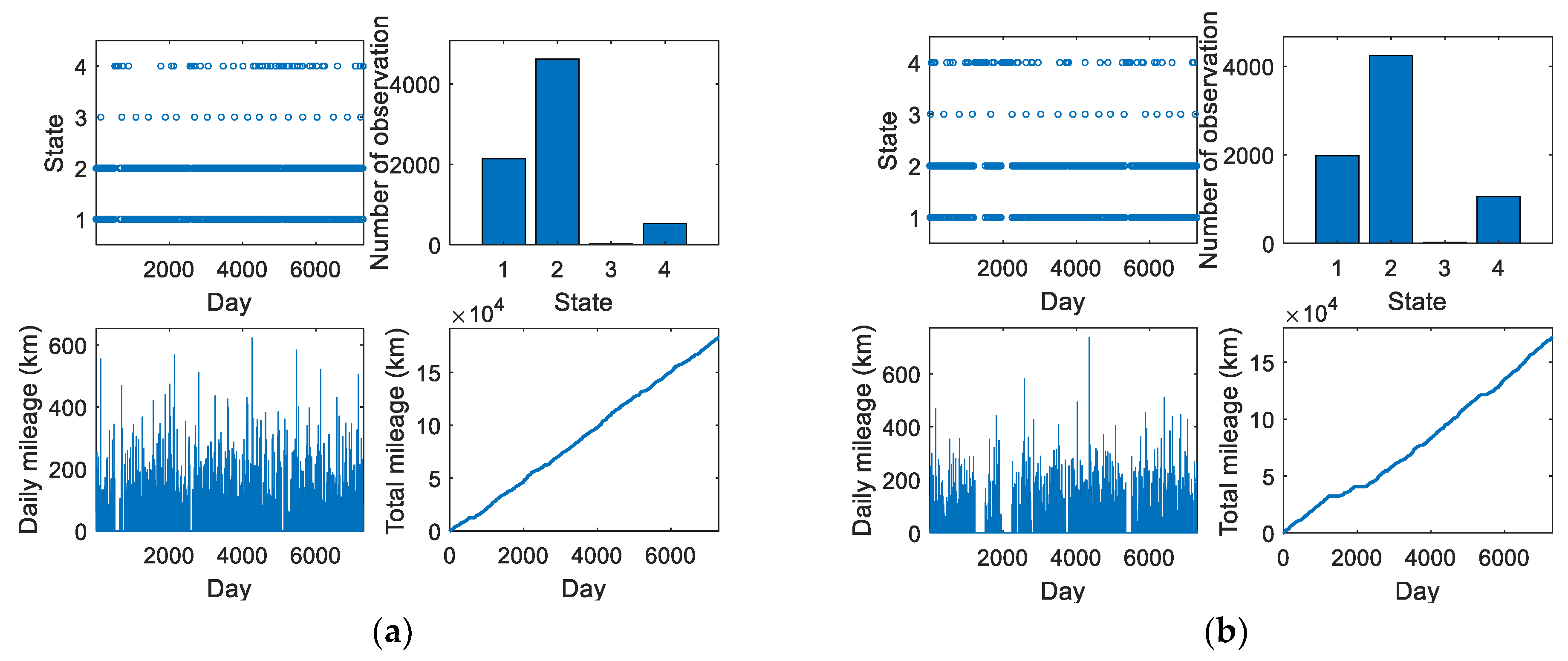
3.5. Monte Carlo Models of Light Utility Vehicle Operation Process

Probabilistic characteristics with a coefficient representing the quality-of-fit to empirical values of at least R = 0.99 were selected to validate the simulation model. Periodic maintenance is the only determined process within the operation system. Transport tasks are assigned according to a binomial distribution with a success probability equal to the value of the Θ coefficient. The exhaustion process of the technical life of the service is measured by the distance covered by a vehicle. Daily mileage is understood as a random variable and is presented as a cumulative distribution function for the exponential, Weibull, lognormal, and gamma distributions. The reliability function is the result of previous research discussed in [12], which involved developing three reliability models. Due to the limitations of the neural model, two other distributions, i.e., exponential and Weibull, are applied to describe the vehicle failure process. On the other hand, the repair process was characterised by Weibull and lognormal distribution functions for the random variable of the time the vehicle was in a state of technical unsuitability.

The general Monte Carlo model developed was validated on the basis of all possible combinations of characteristics exhibited by individual processes that occur within a military transport system.

Table 7. Monte Carlo models of military vehicle operation processes.

Monte Carlo Model	Maintenance	Assignment of Tasks	Operational Process	Reliability	Repair
MC1	Deterministic	Binomial	Exponential	Exponential	Weibull
MC2	Deterministic	Binomial	Exponential	Exponential	Lognormal
MC3	Deterministic	Binomial	Exponential	Weibull	Weibull
MC4	Deterministic	Binomial	Exponential	Weibull	Lognormal
MC5	Deterministic	Binomial	Weibull	Exponential	Weibull
MC6	Deterministic	Binomial	Weibull	Exponential	Lognormal
MC7	Deterministic	Binomial	Weibull	Weibull	Weibull
MC8	Deterministic	Binomial	Weibull	Weibull	Lognormal
MC9	Deterministic	Binomial	Lognormal	Exponential	Weibull
MC10	Deterministic	Binomial	Lognormal	Exponential	Lognormal
MC11	Deterministic	Binomial	Lognormal	Weibull	Weibull
MC12	Deterministic	Binomial	Lognormal	Weibull	Lognormal
MC13	Deterministic	Binomial	Gamma	Exponential	Weibull
MC14	Deterministic	Binomial	Gamma	Exponential	Lognormal
MC15	Deterministic	Binomial	Gamma	Weibull	Weibull
MC16	Deterministic	Binomial	Gamma	Weibull	Lognormal

lists sixteen models with assigned characteristics.

3.6. Software Implementation

A diagram of the proposed method is illustrated in Figure 5. A preliminary stage of simulation implementation is to define the characteristics of processes associated with vehicle operation and to determine the basic simulation parameters, that is, the number of vehicles and the number of iterations conducted. The simulation is then started while the initial value randomisation is maintained for each vehicle.

The first simulation phase involves verifying whether vehicle operating parameters determine periodic maintenance. If this condition is satisfied, the vehicle switches to the S₃ state. Otherwise, a Monte Carlo draw takes place, and it is determined whether a transport task has been assigned for this vehicle to be executed in the simulated step. If such a task is not assigned, the vehicle enters the S₂ state. Otherwise, the simulation draws the daily mileage that the vehicle needs to cover to perform the assigned task. In the next phase, the algorithm checks if there was any vehicle failure during the execution of the task. If such a failure does not occur, the object enters the S₁ state. The appearance of a failure results in classifying the vehicle as being in the S₄ state, where it remains until the repair sub-process is completed.

The proposed method for modelling simulation of a vehicle operation process was implemented within the MATLAB environment. The application pseudocode is shown as Algorithm 1.

Algorithm 1: Pseudocode of Monte Carlo simulation for the four-state operation process.
	Input: Reliability function R(lr), CDF of daily mileage G(ld), probability of assignment task Θ, CDF of repair time H(i), maintenance parameters Lm and Tm, maximum of daily mileage ldmax, number of vehicles Nv, and number of iterations for each vehicle Zi Output: Trajectory X(t), sojourn times T(S1), T(S2), T(S3), T(S4), readiness Kr, and suitability Ks
1	for z = 1: Zi do
2	set t = 1, set random integer values of lm, tm, lr
3	while t ≤ Zi do
4	if lm ≥ Lm then
5	Periodic maintenance X(t) = S3, T(S3) = T(S3) + 1
6	lm = 0, tm = 0
7	t = t + 1
8	elseif tm ≥ Tm then
9	Periodic maintenance X(t) = S3, T(S3) = T(S3) + 1
10	lm = 0, tm = 0
11	t = t + 1
12	else
13	q1 = rand
14	if q1 > Θ then
15	Awaiting for task X(t) = S2, T(S2) = T(S2) + 1
16	t = t + 1
17	else
18	q2 = rand
19	G(ld) = q2, find ld,
20	ld (ld > ldmax) = ldmax
21	q3 = rand
22	if q3 > probability of failure then
23	Task realization X(t) = S1, T(S1) = T(S1) + 1
24	lr = lr + ld, lm = lm + ld, tm = tm + 1
25	t = t + 1
26	else
27	Failure X(t) = S4, T(S4) = T(S4) + 1
28	set random value lf → [0.0, ld]
29	lm = lm + lf, tm = tm + 1
30	t = t + 1
31	q4 = rand
32	i = 1
33	while q4 > probability of repair in i-th iteration do
34	if t < Zi then
35	Repair of vehicle in progress X(t) = S4, T(S4) = T(S4) + 1
36	tm = tm + 1
37	i = i +1
38	q4 = rand
39	t = t + 1
40	else
41	End of simulation; vehicle inoperable
42	end if
43	end while
44	Vehicle repaired in i-th iteration
45	lr = 0
46	t = t + 1
47	end if
48	end if
49	end if
50	end while
51	end for
52	Calculate readiness Kr = [T(S1) + T(S2)]/[T(S1) + T(S2) + T(S3) + T(S4)]
53	Calculate suitability Ks = [T(S1) + T(S2) + T(S3)]/[T(S1) + T(S2) + T(S3) + T(S4)]
54	returnX(t), T(S1), T(S2), T(S3), T(S4), Kr, Ks

4. Semi-Markov Approach

Semi-Markov processes are a generalisation of homogeneous Markov processes in terms of distributions of the individual states’ durations. Markov models assume exponential distributions, significantly narrowing the spectrum of their applications [64]. Furthermore, their use without statistical verification may lead to significant errors in the results obtained, as demonstrated by real case studies in [11,15]. Semi-Markov models are a solution to this problem because they permit distributions of time characteristics [15,65].

The basic description of the semi-Markov process is the Q(t) renewal kernel matrix, consisting of products of the conditional probability p_ij and distribution functions of the condition duration distribution of state S_i prior to transition to state S_j, according to the dependence [66,67]:

$$Q\left(t\right)=\left[\begin{array}{ccccc}0& Q_{12}\left(t\right)& \cdots & Q_{1\left(k-1\right)}\left(t\right)& Q_{1k}\left(t\right)\\ Q_{21}\left(t\right)& 0& \cdots & Q_{2\left(k-1\right)}\left(t\right)& Q_{2k}\left(t\right)\\ ⋮& ⋮& \ddots & ⋮& ⋮\\ Q_{\left(k-1\right)1}\left(t\right)& Q_{\left(k-1\right)2}\left(t\right)& \cdots & 0& Q_{\left(k-1\right)k}\left(t\right)\\ Q_{k1}\left(t\right)& Q_{k2}\left(t\right)& \cdots & Q_{k\left(k-1\right)}\left(t\right)& 0\end{array}\right],$$

(15)

whereas:

$$Q_{ij}\left(t\right)=p_{ij}{F}_{ij}\left(t\right).$$

(16)

where p_ij means the probability of transition from the S_i state to the S_j state and F_ij(t) is the distribution function of time in the S_i state prior to the transition to the S_j state.

An embedded Markov chain is constructed for a semi-Markov process over continuous time. It is a description of the transition states of the process without taking into account the real time in each state. The possibility of a transition from the S_i state to the S_j state is assumed for an embedded Markov chain, provided that i ≠ j. The matrix of conditional probabilities of interstate transitions P may have elements greater than zero only for allowed transitions, which can be written with the formula:

$$P=\left[\begin{array}{ccccc}0& p_{12}& \cdots & p_{1\left(k-1\right)}& p_{1k}\\ p_{21}& 0& \cdots & p_{2\left(k-1\right)}& p_{2k}\\ ⋮& ⋮& \ddots & ⋮& ⋮\\ p_{\left(k-1\right)1}& p_{\left(k-1\right)2}& \cdots & 0& p_{\left(k-1\right)k}\\ p_{k1}& p_{k2}& \cdots & p_{k\left(k-1\right)}& 0\end{array}\right],$$

(17)

under the assumption of meeting the condition of the stochastic matrix [68,69]:

$${\displaystyle \sum _{j=1}^k{p}_{ij}}=1.$$

(18)

Figure 6 shows the transition diagram of the embedded Markov chain for the four-state phase space of operational light utility vehicles. The designations of the states correspond to the assumptions shown in Table 3.

Constructing an embedded Markov chain based on an empirical process waveform implies the need to acquire numerical data on interstate transitions. For this purpose, it is justified to construct a population matrix of interstate transitions N, according to Equation (19) as follows:

$$N=\left[\begin{array}{ccccc}0& n_{12}& \cdots & n_{1\left(k-1\right)}& n_{1k}\\ n_{21}& 0& \cdots & n_{2\left(k-1\right)}& n_{2k}\\ ⋮& ⋮& \ddots & ⋮& ⋮\\ n_{\left(k-1\right)1}& n_{\left(k-1\right)2}& \cdots & 0& n_{\left(k-1\right)k}\\ n_{k1}& n_{k2}& \cdots & n_{k\left(k-1\right)}& 0\end{array}\right].$$

(19)

Values in N matrix correspond to the total number of observed interstate transitions over the analysed process execution time, while n_ij means a transition from S_i to S_j state.

The probability of transitions p_ij in the stochastic matrix P can be acquired by using the values of the population matrix for interstate transitions N by estimating [70,71,72] according to Equation (20) as follows:

$$p_{ij}=\frac{n_{ij}}{{\displaystyle \sum _{j=1}^k{n}_{ij}}},$$

(20)

whereas, the standard estimation errors SE(p_ij) of the probabilities p_ij [73,74] were calculated from formula (21) as follows:

$$SE\left(p_{ij}\right)=\sqrt{\frac{p_{ij}\left(1-p_{ij}\right)}{{\displaystyle {\sum }_{j=1}^n{n}_{ij}}}}.$$

(21)

The values of ergodic probabilities for an embedded Markov chain π_j are calculated by solving the matrix Equation (22) [68] as follows:

$$\left(P^T-I\right)\cdot \Pi =0,$$

(22)

assuming that the standardization condition is met:

$${\displaystyle \sum _{j=1}^n{\pi }_j}=1.$$

(23)

If an embedded Markov chain exhibits ergodicity and there are expected values E(T_i) of state residence times, the values of ergodic probabilities p_j for a semi-Markov process are determined using expression (24) as follows:

$$p_j=\frac{{\pi }_{j}E\left(T_j\right)}{{\displaystyle \sum _{i=1}^n{\pi }_{i}E\left(T_i\right)}}=\frac{{\pi }_j{\displaystyle \sum _{k=1}^n{p}_{jk}E\left(T_{jk}\right)}}{{\displaystyle \sum _{i=1}^n\left({\pi }_i{\displaystyle \sum _{k=1}^n{p}_{ik}E\left(T_{ik}\right)}\right)}},$$

(24)

where π_i is the ergodic probability of an embedded Markov chain for the S_i state and E(T_ik) is the expected value of the direct transition time from the S_i state to the S_k state.

5. Results and Discussion

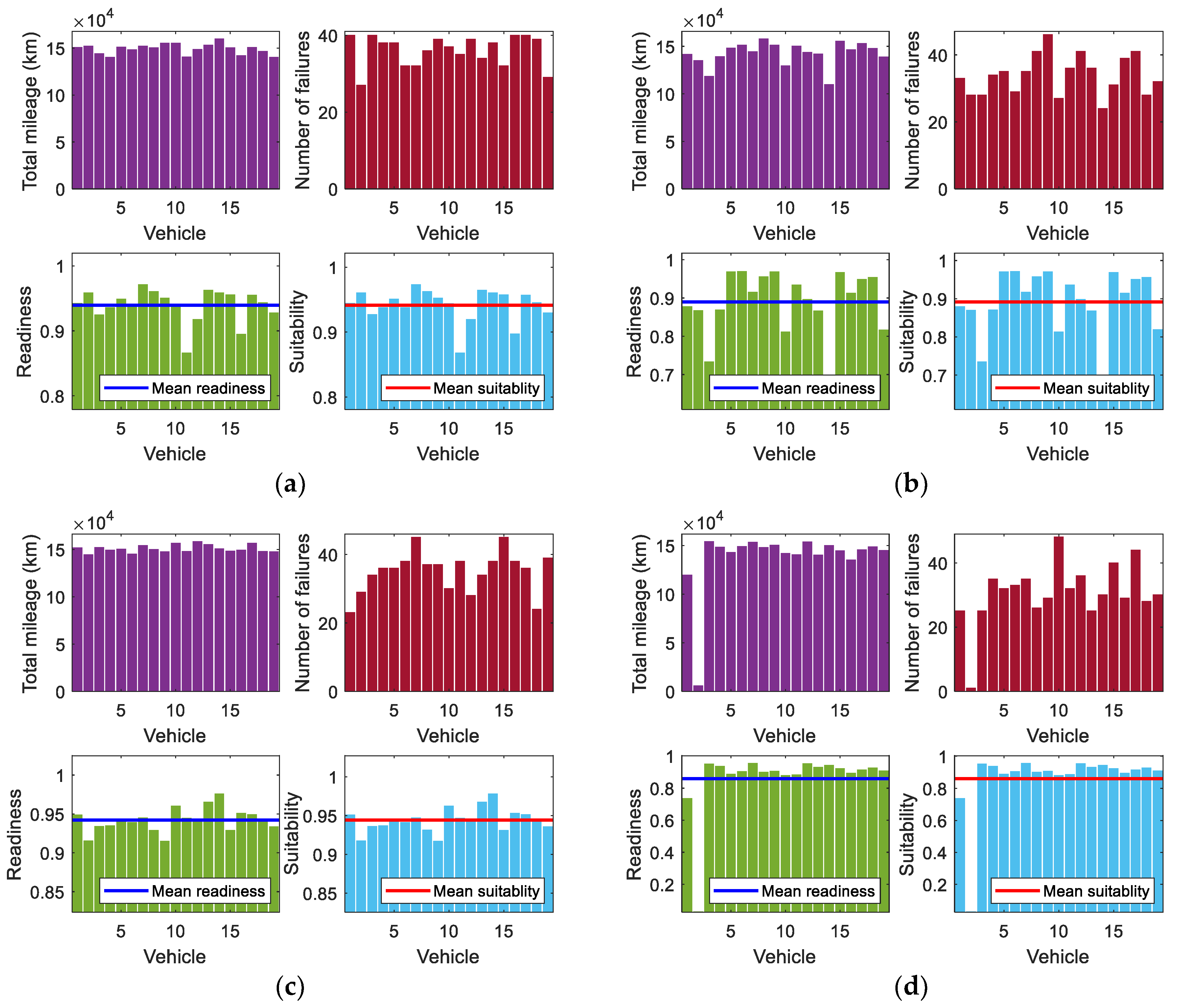
5.1. Monte Carlo Simulations

Simulations were performed for the real operating conditions of the transport system analysed. The operation processes of 19 light utility vehicles were simulated over a predicted 20-year operation period as set out in operational standards for each of the 16 Monte Carlo models [52]. Figure 7 shows sample waveforms of the simulated operation process for selected vehicles and Monte Carlo models.

The simulated operation of individual vehicles may show clearly different courses. Repairs of vehicles No. 4 in MC1 and No. 13 in MC6 took place shortly after a failure occurred. On the contrary, vehicle No. 19 in MC10 and No. 14 in MC14, after several failures, remained in an unsuitable state for a prolonged time, which adversely affected the object readiness index values.

Figure 8a–d shows detailed simulation results of the MC1 model. During a 20-year operation period, all vehicles must cover distances in the range of 150,000.0 to 200,000.0 km, which is shown in Figure 8a. In reference to the operational potential specified in the Catalogue of Operational Standards at a level of 230,000.0 km, our work reveals that the current operation intensity can be maintained for the entire estimated operation period. Furthermore, the number of failures for individual objects (Figure 8b) fell within the range of 30 to 60, while the average number of failures per vehicle was 45.68. Functional readiness and technical suitability were quite varied, with each vehicle exhibiting values of the K_r and K_s indices greater than 0.80, as illustrated in Figure 8c,d. The simulation results of all models (MC1–MC16) are presented in Appendix A.

5.2. Semi-Markov Model

An estimation of the conditional transition probability matrix was carried out using Equations (17)–(20), based on data collected from the real operation process of 19 light utility vehicles. During a 3-year period of operation, 7763 interstate transitions were observed for the study sample, whereas the numbers of transitions between states were represented by the N matrix:

$$N=\left[\begin{array}{cccc}0& 3641& 27& 94\\ 3729& 0& 70& 0\\ 9& 97& 0& 0\\ 24& 63& 9& 0\end{array}\right].$$

(25)

The result of the estimation is the P matrix presented below:

$$P=\left[\begin{array}{cccc}0& 0.9678& 0.0072& 0.0250\\ 0.9816& 0& 0.0184& 0\\ 0.0849& 0.9151& 0& 0\\ 0.2500& 0.6562& 0.0938& 0\end{array}\right].$$

(26)

According to Equation (21), with an increase in the number of transitions from the S_i state, the standard error SE(p_ij) decreases. For this reason, the standard error is higher for operational states in which the technical object has been observed to be relatively rare. However, for all conditional probabilities, the SE(p_ij) did not exceed the value of 0.05, as shown in Equation (27), so the results are considered acceptable [15,75,76].

$$SE=\left[\begin{array}{cccc}0& 0.0029& 0.0014& 0.0025\\ 0.0022& 0& 0.0022& 0\\ 0.0271& 0.0271& 0& 0\\ 0.0442& 0.0485& 0.0297& 0\end{array}\right].$$

(27)

The expected values of the interstate transition times E(T_ij) were estimated as arithmetic averages of the empirical transition times, which are represented by the T matrix (28):

$$T=\left[\begin{array}{cccc}0& 12.63& 2.23& 14.00\\ 72.23& 0& 129.5& 0\\ 187.03& 4.44& 0& 0\\ 16.28& 518.84& 124.98& 0\end{array}\right].$$

(28)

The ergodic probabilities π_j of the embedded Markov chain were calculated using the matrix equation (29) with the normalisation condition (23) as follows:

$$\left(P^T-I\right)\cdot \Pi =\left[\begin{array}{cccc}-1& 0.9678& 0.0072& 0.0250\\ 0.9816& -1& 0.0184& 0\\ 0.0849& 0.9151& -1& 0\\ 0.2500& 0.6562& 0.0938& -1\end{array}\right]\cdot \left[\begin{array}{c}{\pi }_1\\ {\pi }_2\\ {\pi }_3\\ {\pi }_4\end{array}\right]=\left[\begin{array}{c}0\\ 0\\ 0\\ 0\end{array}\right].$$

(29)

Then, based on the probabilities p and the times E(T_ij), the ergodic probability values p_j of the semi-Markov model were calculated using the relation (24). Figure 9a,b shows the results of the calculations for the embedded Markov chain and the SMM, respectively.

The π_j values of the embedded Markov chain contain information about the frequency of occurrence of states in the operation process without taking into account the time duration. In these terms, the most frequent states are S₁ and S₂, each above 48%. The SMM p_j values refer to the temporal stay of vehicles in states S₁–S₄, which is the basis for the calculation of readiness and suitability indices. At random time t, the vehicle will be in state S₂ with the highest probability (more than 77%).

5.3. Comparison of the Results

The results of all the simulations are in

Table 8. Simulation and results of the semi-Markov model.

Simulation	Readiness Kr			Suitability Ks
	Monte Carlo	Semi-Markov	Percentage Error (%)	Monte Carlo	Semi-Markov	Percentage Error (%)
MC1	0.9078	0.9015	0.70	0.9104	0.9073	0.34
MC2	0.8766	0.9015	−2.76	0.8790	0.9073	−3.12
MC3	0.9337	0.9015	3.57	0.9363	0.9073	3.20
MC4	0.9195	0.9015	2.00	0.9221	0.9073	1.63
MC5	0.9142	0.9015	1.41	0.9167	0.9073	1.04
MC6	0.8735	0.9015	−3.11	0.8760	0.9073	−3.45
MC7	0.9329	0.9015	3.48	0.9355	0.9073	3.11
MC8	0.8791	0.9015	−2.48	0.8816	0.9073	−2.83
MC9	0.9163	0.9015	1.64	0.9189	0.9073	1.28
MC10	0.8545	0.9015	−5.21	0.8571	0.9073	−5.53
MC11	0.9257	0.9015	2.68	0.9284	0.9073	2.33
MC12	0.8727	0.9015	−3.19	0.8753	0.9073	−3.53
MC13	0.9393	0.9015	4.19	0.9414	0.9073	3.76
MC14	0.8895	0.9015	−1.33	0.8916	0.9073	−1.73
MC15	0.9419	0.9015	4.48	0.9440	0.9073	4.04
MC16	0.8597	0.9015	−4.64	0.8617	0.9073	−5.03

. The values of the readiness and technical suitability indicators were compared with the results of the semi-Markov models (SMM). The ergodic probabilities determined for a four-state SMM constituted grounds to determine functional readiness and technical suitability indices, which reached values of 0.9015 and 0.9073, respectively. The results of all simulation models did not differ from SMM by more than 6%, which demonstrates the high precision of the developed models. Given the above, MC1 turned out to be the best four-state model. Its readiness and suitability indices differed from the boundary values of the semi-Markov model by 0.70% and 0.34%, respectively.

The relatively low frequency of maintenance and service leads to minor differences between the K_r readiness index and the K_s suitability index. From the perspective of vehicle operation and satisfying transport needs, the K_r readiness index is very important.

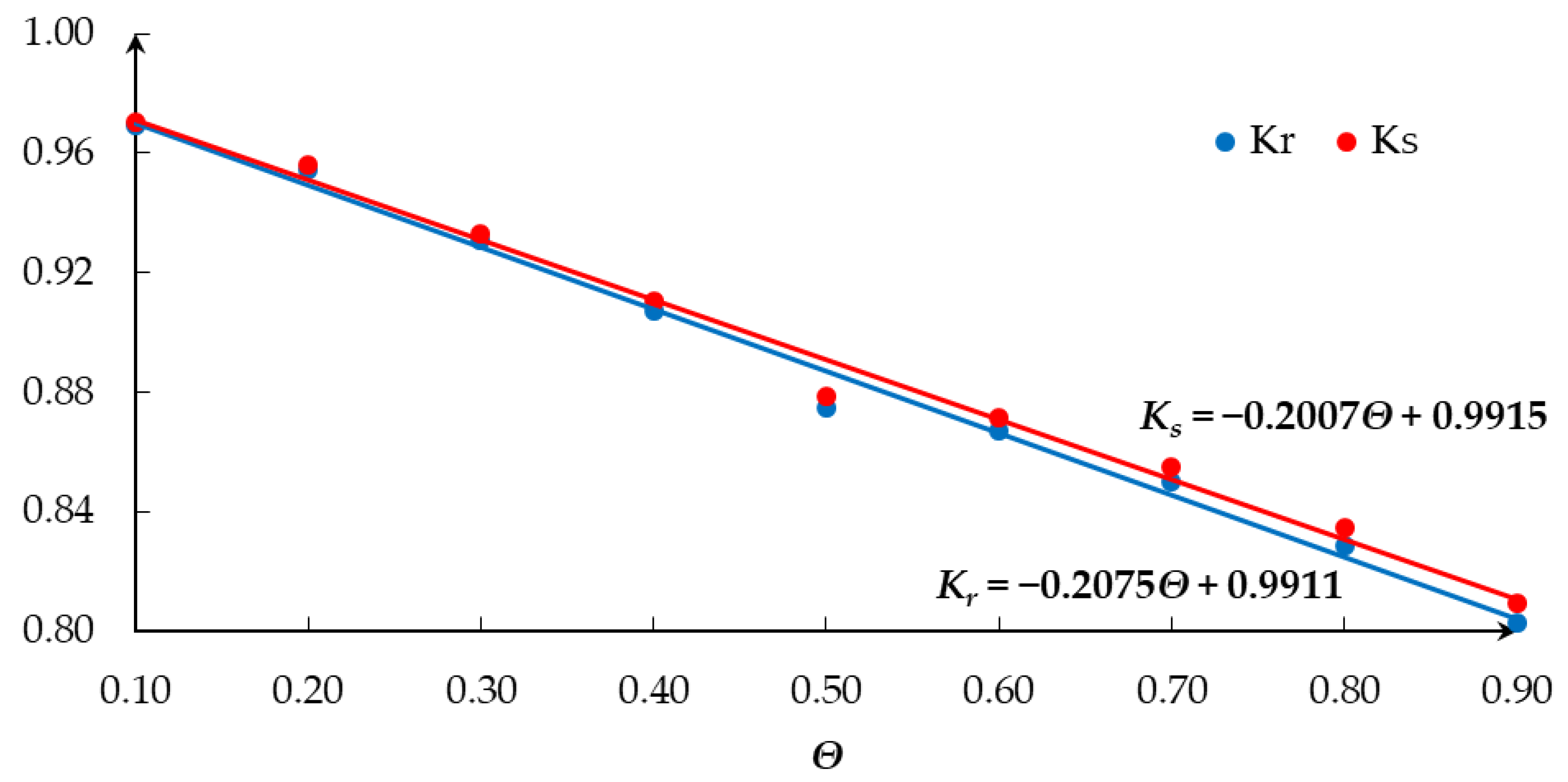
5.4. Functional Readiness

Functional readiness defines the probability that a technical object will remain in a state of technical suitability where it can fully implement tasks according to its intended use. Figure 10 shows a functional readiness graph for a car fleet on individual days throughout a simulated operation process. It was defined as a percentage of vehicles in either state S₁ or S₂. Maintaining the K_r(t) indices at an adequately high level is significant from the perspective of safely providing the transport capacity for the operational system. Within the simulation, this index took on a value of 0.55–0.70 through its several iterations. Therefore, more than 70% of the vehicles were ready for operation within the transport system for most of the operation period.

The analysis covered the impact of the number of iterations of the simulated process of operating 19 vehicles that form a transport system according to functional readiness. Figure 11 shows the mean value of the K_r index within the measured iteration range [0, t], while t consecutively takes the values of integers in the range of [1, 7300]. At the initial stage of the simulation, functional readiness was found to remain high and then started to decline. After conducting more than 1000 iterations, the K_r index began to gradually stabilise at a level of approximately 0.91. This value came about due to the occurrence of recorded failures and, consequently, damaged vehicles remaining in the state of technical unsuitability.

5.5. Sensitivity Analysis of Monte Carlo Model

A sensitivity analysis of the MC1 model was conducted in order to determine the impact of functional readiness and technical suitability indices depending on the intensity of vehicle operation. The intensity operation is defined by the probability of assigning the transport task Θ and the expected daily mileage value during the execution of the task. The simulated operation process was implemented for specified ranges of considered variables, while at the same time, maintaining the true characteristics of other sub-processes.

Table 9. Readiness and suitability indicators obtained by sensitivity analysis of the Θ index.

Θ	Kr	Ks
0.10	0.9695	0.9704
0.20	0.9547	0.9564
0.30	0.9309	0.9333
0.40	0.9073	0.9104
0.50	0.8750	0.8788
0.60	0.8670	0.8715
0.70	0.8501	0.8553
0.80	0.8289	0.8347
0.90	0.8031	0.8094
0.10	0.9695	0.9704

shows the results of the sensitivity analysis for the Θ coefficient, which takes values from the range [0.10–0.90]. With the minimum vehicle utilisation rate at an average level of 10% of vehicles per day, the daily functional readiness and technical suitability indices reached values of approximately 0.97. However, with an increase in the number of daily operated vehicles, these indices decline until reaching values of approximately 0.80 for a probability of 90% for transport task allocation. Figure 12 shows linear approximations of the K_r and K_s indices depending on the Θ coefficient, carried out using the least squares method. The match of linear approximating functions with simulated data was R² = 0.9916 for the K_r index and R² = 0.9910 for the K_s index. According to the approximate functions, an increase in the Θ coefficient by 0.01 leads to a reduction in the values of the indices K_r and K_s by approximately 0.002.

Table 10. Readiness and suitability indicators obtained by sensitivity analysis of expected daily mileage.

Expected Daily Mileage (km)	Kr	Ks
50	0.9445	0.9461
60	0.9476	0.9495
70	0.9431	0.9452
80	0.9348	0.9371
90	0.9097	0.9123
100	0.9094	0.9122
110	0.9049	0.9080
120	0.8993	0.9027
130	0.8838	0.8873
140	0.8768	0.8806
150	0.8735	0.8775

lists the results of the sensitivity analysis for the expected daily mileage l_d over a variability range of 50.0–150.0 km. Figure 13 shows linear approximations of the K_r and K_s indices depending on the expected daily mileage l_d, which exhibited fit to the simulated data at a level of R² = 0.9580 and R² = 0.9554, respectively. In this paper, an increase in the expected daily mileage by 1.0 km leads to a decrease in the value of the functional readiness and technical suitability indices by approximately 0.0008.

6. Conclusions

This article presents an original Monte Carlo operation process simulation model for light utility vehicles operated by a military transport system. Based on an analysis of the empirical course of the process and the results of previous research, the authors identified a four-state phase space. The planned and preventive strategy for operational management introduces a deterministic element occurring within the stochastic process of changes in the operational state. In the case of military vehicles, the deterministic element is the frequency of periodic maintenance and service defined in the vehicle operation manual and the catalogue of operational standards.

The theoretical simulation model was implemented within the MATLAB software. Its validation was based on probabilistic characteristics estimated on the basis of empirical data. In this work, the simulated course of a stochastic process for 19 vehicles over a predicted 20-year operation period allowed the estimation of the functional readiness index and technical suitability index values in the range of [0.8545–0.9419] and [0.8571–0.9440], respectively. The relative differences between the results of 16 simulation models and the semi-Markov model were less than 6%. Therefore, this minor disproportion confirms the high usefulness of Monte Carlo methods for modelling the operation process.

Moreover, unlike Markov and semi-Markov models, Monte Carlo methods enable consideration of the behaviour of a technical object in hypothetical scenarios that are different from standard operating conditions. This consideration allows for extrapolating the obtained results. The case study involved analysing the sensitivity of the best-fit MC1 model in terms of the impact of vehicle operation intensity on the values of the K_r and K_s coefficients. Based on the spot results of the analyses, the authors performed an approximation with linear functions using the least squares method. Accordingly, an increase in the operation utilisation coefficient of 0.01 entails a decrease in the K_r and K_s coefficient by an average of approximately 0.002. On the other hand, an increase in expected daily mileage according to an exponential distribution of 1.0 km generates a decrease in the K_r and K_s coefficients of approximately 0.008.

An undoubted advantage of the proposed model is the relatively small set of empirical data required for its validation. The assumption of process discretization related to both states (four states) and time (single-day time intervals) implies the need to learn the probabilistic characteristics that determine changes in operational states. The adopted assumptions lead to a simplification of the analysed process, which results in omitting short-term situations and states that are insignificant from the perspectives of both functional readiness and technical suitability.

The proposed approach based on the iterative Monte Carlo algorithm can be implemented in both military and civilian transport systems, as well as industrial machinery. A practical aspect of the algorithm’s application is the ability to assess and predict the readiness and suitability of technical objects and systems.

The developed simulation model does not take into account the seasonality of the operation process. Seasonal fluctuations may concern the sub-process of operation, periodic maintenance, and repair implementation. In addition, the social life cycle significantly impacts the intensity of vehicle operation on non-working days (Saturdays and Sundays) relative to other days of the week. A similar phenomenon is associated with maintenance and repair sub-processes, which are implemented primarily from Monday to Friday. The proposed Monte Carlo model does not classify successive iterations as individual days of the week. Expanding the developed model will be the direction of further research within this field.

References

1. Benson, R.; Kellner, D. Monte Carlo Simulation for Reliability. In Proceedings of the 2020 Annual Reliability and Maintainability Symposium (RAMS), Palm Springs, CA, USA, 27–30 January 2020; pp. 1–6. [Google Scholar]
2. Acebes, F.; Poza, D.; González-Varona, J.M.; López-Paredes, A. Stochastic Earned Duration Analysis for Project Schedule Management. Engineering 2022, 9, 148–161. [Google Scholar] [CrossRef]
3. Dąbrowska, E. Monte Carlo Simulation Approach to Reliability Analysis of Complex Systems. J. Konbin 2020, 50, 155–170. [Google Scholar] [CrossRef]
4. Ren, W.; Ma, L.; Wang, Y. Monte Carlo Analysis for Safety and Reliability of Rail Transit Signal System Based on Cloud Computing. J. Phys. Conf. Ser. 2020, 1654, 012065. [Google Scholar] [CrossRef]
5. Liu, C.; Kramer, A.; Neumann, S. Reliability Assessment of Repairable Phased-Mission System by Monte Carlo Simulation Based on Modular Sequence-Enforcing Fault Tree Model. Eksploat. I Niezawodn. Maint. Reliab. 2020, 22, 272–281. [Google Scholar] [CrossRef]
6. Amjad, M.; Ahmad, I.; Ahmad, M.; Wróblewski, P.; Kamiński, P.; Amjad, U. Prediction of Pile Bearing Capacity Using XGBoost Algorithm: Modeling and Performance Evaluation. Appl. Sci. 2022, 12, 2126. [Google Scholar] [CrossRef]
7. Janekova, J.; Fabianova, J.; Kadarova, J. Selection of Optimal Investment Variant Based on Monte Carlo Simulations. Int. J. Simul. Model. 2021, 20, 279–290. [Google Scholar] [CrossRef]
8. Żurek, J.; Zieja, M.; Ziółkowski, J.; Borucka, A. Vehicle Operation Process Analysis Using the Markov Processes. In Proceedings of the 29th European Safety and Reliability Conference, Hannover, Germany, 22–26 September 2019; pp. 2598–2605. [Google Scholar]
9. Ziółkowski, J.; Borucka, A. Markov Model in Logistic Management of Enterprise. J. Konbin 2016, 38, 271–290. [Google Scholar] [CrossRef] [Green Version]
10. Borucka, A.; Niewczas, A.; Hasilova, K. Forecasting the Readiness of Special Vehicles Using the Semi-Markov Model. Eksploat. Niezawodn. Maint. Reliab. 2019, 21, 662–669. [Google Scholar] [CrossRef]
11. Świderski, A.; Borucka, A.; Grzelak, M.; Gil, L. Evaluation of Machinery Readiness Using Semi-Markov Processes. Appl. Sci. 2020, 10, 1541. [Google Scholar] [CrossRef] [Green Version]
12. Oszczypała, M.; Ziółkowski, J.; Małachowski, J. Reliability Analysis of Military Vehicles Based on Censored Failures Data. Appl. Sci. 2022, 12, 2622. [Google Scholar] [CrossRef]
13. Dziubak, T.; Wysocki, T.; Dziubak, S. Selection of Vehicles for Fleet of Transport Company on the Basis of Observation of Their Operational Reliability. Eksploat. Niezawodn. Maint. Reliab. 2021, 23, 184–194. [Google Scholar] [CrossRef]
14. Żurek, J.; Ziółkowski, J.; Borucka, A. Application of Markov Processes to the Method for Analysis of Combat Vehicle Operation in the Aspect of Their Availability and Readiness. In Proceedings of the 2nd International Conference on Engineering Sciences and Technologies, Kerbala, Iraq, 26–28 March 2018; pp. 2343–2352. [Google Scholar]
15. Oszczypała, M.; Ziółkowski, J.; Małachowski, J. Analysis of Light Utility Vehicle Readiness in Military Transportation Systems Using Markov and Semi-Markov Processes. Energies 2022, 15, 5062. [Google Scholar] [CrossRef]
16. Liu, K.; Wu, J.; Liu, H.; Sun, M.; Wang, Y. Reliability Analysis of Thermal Error Model Based on DBN and Monte Carlo Method. Mech. Syst. Signal Process. 2021, 146, 107020. [Google Scholar] [CrossRef]
17. Jensen, H.A.; Jerez, D.J.; Valdebenito, M. An Adaptive Scheme for Reliability-Based Global Design Optimization: A Markov Chain Monte Carlo Approach. Mech. Syst. Signal Process. 2020, 143, 106836. [Google Scholar] [CrossRef]
18. Zhang, L.; Dong, L.; Cheng, S.; Li, W.; Wang, B.; Liu, H.; Chen, K. Efficient Reliability Assessment Method for Bridges Based on Markov Chain Monte Carlo (MCMC) with Metropolis-Hasting Algorithm (MHA). IOP Conf. Ser. Earth Environ. Sci. 2020, 580, 012030. [Google Scholar] [CrossRef]
19. Zhu, H.; Wang, X.; Xiao, M.; Yang, Z.; Tang, X.; Wen, B. Reliability Modeling for Intermittent Working System Based on Wiener Process. Comput. Ind. Eng. 2021, 160, 107599. [Google Scholar] [CrossRef]
20. Shahtaheri, Y.; Flint, M.M.; De la Garza, J.M. A Multi-Objective Reliability-Based Decision Support System for Incorporating Decision Maker Utilities in the Design of Infrastructure. Adv. Eng. Inform. 2019, 42, 100939. [Google Scholar] [CrossRef]
21. Zhang, K.; Tang, B.; Deng, L.; Yu, X.; Wei, J. Fault Source Location of Wind Turbine Based on Heterogeneous Nodes Complex Network. Eng. Appl. Artif. Intell. 2021, 103, 104300. [Google Scholar] [CrossRef]
22. Kallen, M.J. Modelling Imperfect Maintenance and the Reliability of Complex Systems Using Superposed Renewal Processes. Reliab. Eng. Syst. Saf. 2011, 96, 636–641. [Google Scholar] [CrossRef]
23. Durczak, K.; Rybacki, P.; Sujak, A. Application of a Selected Pseudorandom Number Generator for the Reliability of Farm Tractors. Appl. Sci. 2022, 12, 12452. [Google Scholar] [CrossRef]
24. Singh, C.; Mitra, J. Monte Carlo Simulation for Reliability Analysis of Emergency and Standby Power Systems. In Proceedings of the IAS ’95. Conference Record of the 1995 IEEE Industry Applications Conference Thirtieth IAS Annual Meeting, Orlando, FL, USA, 8–12 October 1995; Volume 3, pp. 2290–2295. [Google Scholar]
25. Souza-Franco, R.L.; Clavijo, V.; Schleder, M.; Martins, R. Monte Carlo Simulation to Consider Uncertainty in the Reliability Analysis of Dynamic Positioning Systems. In Proceedings of the 29th European Safety and Reliability Conference (ESREL), Hannover, Germany, 22–26 September 2019; Research Publishing Services: Hannover, Germany, 2019; pp. 2446–2453. [Google Scholar]
26. Novak, M.; Sangwongwanich, A.; Blaabjerg, F. Monte Carlo Based Reliability Estimation Methods in Power Electronics. In Proceedings of the 2020 IEEE 21st Workshop on Control and Modeling for Power Electronics (COMPEL), Aalborg, Denmark, 9–12 November 2020; pp. 1–7. [Google Scholar]
27. Green, R.C.; Wang, L.; Alam, M.; Singh, C. Intelligent State Space Pruning for Monte Carlo Simulation with Applications in Composite Power System Reliability. Eng. Appl. Artif. Intell. 2013, 26, 1707–1724. [Google Scholar] [CrossRef]
28. Roslan, N.N.R.B.; Fauzi, N.F.B.M.; Ridzuan, M.I.M. Sequential and Nonsequential Monte Carlo in Assessing Reliability Performance of Distribution Network. In Proceedings of the 2020 Emerging Technology in Computing, Communication and Electronics (ETCCE), Dhaka, Bangladesh, 21–22 December 2020; pp. 1–6. [Google Scholar]
29. Ugurlu, O.F.; Kumral, M. Reliability-Based Performance Analysis of Mining Drilling Operations through Markov Chain Monte Carlo and Mean Reverting Process Simulations. Simulation 2020, 96, 593–604. [Google Scholar] [CrossRef]
30. Hu, Y.-W.; Zhang, H.-C.; Liu, S.-J.; Lu, H.-T. Sequential Monte Carlo Method Toward Online RUL Assessment with Applications. Chin. J. Mech. Eng. 2018, 31, 5. [Google Scholar] [CrossRef]
31. Sharma, S.; Cui, Y.; He, Q.; Mohammadi, R.; Li, Z. Data-Driven Optimization of Railway Maintenance for Track Geometry. Transp. Res. Part C Emerg. Technol. 2018, 90, 34–58. [Google Scholar] [CrossRef]
32. Zhang, X.; Lu, Z.; Cheng, K.; Wang, Y. A Novel Reliability Sensitivity Analysis Method Based on Directional Sampling and Monte Carlo Simulation. Proc. Inst. Mech. Eng. Part O J. Risk Reliab. 2020, 234, 622–635. [Google Scholar] [CrossRef]
33. Zhang, K.; Du, Z.; Xiao, F.; Wang, T.; Zhang, L. Improved Sequential Monte Carlo Method Approach to Substation Connection Reliability Assessment. In Proceedings of the 2020 IEEE 4th Conference on Energy Internet and Energy System Integration (EI2), Wuhan, China, 30 October–1 November 2020; pp. 2357–2362. [Google Scholar]
34. Macheret, Y.; Koehn, P.; Sparrow, D. Improving Reliability and Operational Availability of Military Systems. In Proceedings of the 2005 IEEE Aerospace Conference, Big Sky, MT, USA, 5–12 March 2003; IEEE Operations Center: Big Sky, MT, USA, 2005; pp. 3948–3957. [Google Scholar]
35. Andrade-Michel, A.; Ríos-Solís, Y.A.; Boyer, V. Vehicle and Reliable Driver Scheduling for Public Bus Transportation Systems. Transp. Res. Part B Methodol. 2021, 145, 290–301. [Google Scholar] [CrossRef]
36. Wang, Y.; Infield, D. Markov Chain Monte Carlo Simulation of Electric Vehicle Use for Network Integration Studies. Int. J. Electr. Power Energy Syst. 2018, 99, 85–94. [Google Scholar] [CrossRef]
37. Ricard, L.; Desaulniers, G.; Lodi, A.; Rousseau, L.-M. Predicting the Probability Distribution of Bus Travel Time to Measure the Reliability of Public Transport Services. Transp. Res. Part C Emerg. Technol. 2022, 138, 103619. [Google Scholar] [CrossRef]
38. Salgado Duarte, Y.; Szpytko, J.; Del Castillo Serpa, A.M. Monte Carlo Simulation Model to Coordinate the Preventive Maintenance Scheduling of Generating Units in Isolated Distributed Power Systems. Electr. Power Syst. Res. 2020, 182, 106237. [Google Scholar] [CrossRef]
39. Lojowska, A.; Kurowicka, D.; Papaefthymiou, G.; van der Sluis, L. Stochastic Modeling of Power Demand Due to EVs Using Copula. IEEE Trans. Power Syst. 2012, 27, 1960–1968. [Google Scholar] [CrossRef]
40. Paś, J.; Klimczak, T.; Rosiński, A.; Stawowy, M. The Analysis of the Operational Process of a Complex Fire Alarm System Used in Transport Facilities. Build. Simul. 2022, 15, 615–629. [Google Scholar] [CrossRef]
41. Stawowy, M.; Rosiński, A.; Siergiejczyk, M.; Perlicki, K. Quality and Reliability-Exploitation Modeling of Power Supply Systems. Energies 2021, 14, 2727. [Google Scholar] [CrossRef]
42. Borowski, S.; Szubartowski, M.; Migawa, K.; Sołtysiak, A.; Neubauer, A.; Hujo, L.; Nosian, J. Mathematical Model for Determining the Time of Preventive Replacements in the Agricultural Machinery Service System with Minimal Repair. Appl. Sci. 2023, 13, 640. [Google Scholar] [CrossRef]
43. Migawa, K.; Borowski, S.; Neubauer, A.; Sołtysiak, A. Semi-Markov Model of the System of Repairs and Preventive Replacements by Age of City Buses. Appl. Sci. 2021, 11, 10411. [Google Scholar] [CrossRef]
44. Liu, P.; Wang, G. Optimal Periodic Preventive Maintenance Policies for Systems Subject to Shocks. Appl. Math. Model. 2021, 93, 101–114. [Google Scholar] [CrossRef]
45. Park, M.; Jung, K.M.; Park, D.H. Optimization of Periodic Preventive Maintenance Policy Following the Expiration of Two-Dimensional Warranty. Reliab. Eng. Syst. Saf. 2018, 170, 1–9. [Google Scholar] [CrossRef]
46. Hu, J.; Shen, J.; Shen, L. Periodic Preventive Maintenance Planning for Systems Working under a Markovian Operating Condition. Comput. Ind. Eng. 2020, 142, 106291. [Google Scholar] [CrossRef]
47. Wang, W.; Wu, Z.; Xiong, J.; Xu, Y. Redundancy Optimization of Cold-Standby Systems under Periodic Inspection and Maintenance. Reliab. Eng. Syst. Saf. 2018, 180, 394–402. [Google Scholar] [CrossRef]
48. Adekitan, A.I.; Bukola, A.; Kennedy, O. A Data-Based Investigation of Vehicle Maintenance Cost Components Using ANN. IOP Conf. Ser. Mater. Sci. Eng. 2018, 413, 012009. [Google Scholar] [CrossRef]
49. Chen, C.; Liu, Y.; Wang, S.; Sun, X.; Di Cairano-Gilfedder, C.; Titmus, S.; Syntetos, A.A. Predictive Maintenance Using Cox Proportional Hazard Deep Learning. Adv. Eng. Inform. 2020, 44, 101054. [Google Scholar] [CrossRef]
50. Hu, J.; Wang, Y.; Pang, Y.; Liu, Y. Optimal Maintenance Scheduling under Uncertainties Using Linear Programming-Enhanced Reinforcement Learning. Eng. Appl. Artif. Intell. 2022, 109, 104655. [Google Scholar] [CrossRef]
51. Sbihi, M.; Varnier, C. Single-Machine Scheduling with Periodic and Flexible Periodic Maintenance to Minimize Maximum Tardiness. Comput. Ind. Eng. 2008, 55, 830–840. [Google Scholar] [CrossRef] [Green Version]
52. Ministry of Defense of Poland. DTU-4.22.13.1(A). Catalog of Operating Norms for Land Machinery; Ministry of Defense of Poland; Armed Forces Support Inspectorate: Bydgoszcz, Poland, 2019.
53. Redmer, A. Optimisation of the Exploitation Period of Individual Vehicles in Freight Transportation Companies. Transp. Res. Part E Logist. Transp. Rev. 2009, 45, 978–987. [Google Scholar] [CrossRef]
54. Betkier, I.; Macioszek, E. Characteristics of Parking Lots Located along Main Roads in Terms of Cargo Truck Requirements: A Case Study of Poland. Sustainability 2022, 14, 15720. [Google Scholar] [CrossRef]
55. Soltanali, H.; Rohani, A.; Abbaspour-Fard, M.H.; Farinha, J.T. A Comparative Study of Statistical and Soft Computing Techniques for Reliability Prediction of Automotive Manufacturing. Appl. Soft Comput. 2021, 98, 106738. [Google Scholar] [CrossRef]
56. Gołda, P.; Zawisza, T.; Izdebski, M. Evaluation of Efficiency and Reliability of Airport Processes Using Simulation Tools. Eksploat. Niezawodn. 2021, 23, 659–669. [Google Scholar] [CrossRef]
57. Wang, J.; Gao, X.; Sun, Z. An Importance Sampling Framework for Time-Variant Reliability Analysis Involving Stochastic Processes. Sustainability 2021, 13, 7776. [Google Scholar] [CrossRef]
58. Alkaff, A.; Qomarudin, M.N.; Purwantini, E.; Wiratno, S.E. Dynamic Reliability Modeling for General Standby Systems. Comput. Ind. Eng. 2021, 161, 107615. [Google Scholar] [CrossRef]
59. Hao, S.; Yang, J.; Ma, X.; Zhao, Y. Reliability Modeling for Mutually Dependent Competing Failure Processes Due to Degradation and Random Shocks. Appl. Math. Model. 2017, 51, 232–249. [Google Scholar] [CrossRef]
60. Hong, L.; Zhai, Q.; Wang, X.; Ye, Z.-S. System Reliability Evaluation Under Dynamic Operating Conditions. IEEE Trans. Reliab. 2019, 68, 800–809. [Google Scholar] [CrossRef]
61. Torii, A.J.; Novotny, A.A. A Priori Error Estimates for Local Reliability-Based Sensitivity Analysis with Monte Carlo Simulation. Reliab. Eng. Syst. Saf. 2021, 213, 107749. [Google Scholar] [CrossRef]
62. Angus, J.; Ding, Y. On the Ratio of Current Age to Total Life for Null Recurrent Renewal Processes. Stat. Probab. Lett. 2020, 162, 399. [Google Scholar] [CrossRef]
63. Vassiliou, P.-C.G. Non-Homogeneous Semi-Markov and Markov Renewal Processes and Change of Measure in Credit Risk. Mathematics 2020, 9, 55. [Google Scholar] [CrossRef]
64. Ziółkowski, J.; Małachowski, J.; Oszczypała, M.; Szkutnik-Rogoż, J.; Lęgas, A. Modelling of the Military Helicopter Operation Process in Terms of Readiness. Def. Sci. J. 2021, 71, 602–611. [Google Scholar] [CrossRef]
65. Grabski, F. Semi-Markov Failure Rates Processes. Appl. Math. Comput. 2011, 217, 9956–9965. [Google Scholar] [CrossRef]
66. Migawa, K. Availability Control for Means of Transport in Decisive Semi-Markov Models of Exploitation Process. Arch. Transp. 2012, 24, 497–508. [Google Scholar] [CrossRef] [Green Version]
67. Ivanchenko, O.; Kharchenko, V.; Moroz, B.; Kabak, L.; Smoktii, K. Semi-Markov Availability Model Considering Deliberate Malicious Impacts on an Infrastructure-as-a-Service Cloud. In Proceedings of the 2018 14th International Conference on Advanced Trends in Radioelectronics, Telecommunications and Computer Engineering (TCSET), Lviv-Slavske, Ukraine, 20–24 February 2018; pp. 570–573. [Google Scholar]
68. Karakaya, E.; Vinel, A.; Smith, A.E. Relocations in Container Depots for Different Handling Equipment Types: Markov Models. Comput. Ind. Eng. 2021, 157, 107311. [Google Scholar] [CrossRef]
69. Oniszczuk, W. Loss Tandem Networks with Blocking—A Semi-Markov Approach. Bull. Pol. Acad. Sci. Tech. Sci. 2010, 58, 673–681. [Google Scholar] [CrossRef]
70. Shepero, M.; Munkhammar, J. Spatial Markov Chain Model for Electric Vehicle Charging in Cities Using Geographical Information System (GIS) Data. Appl. Energy 2018, 231, 1089–1099. [Google Scholar] [CrossRef]
71. Iversen, E.B.; Morales, J.M.; Madsen, H. Optimal Charging of an Electric Vehicle Using a Markov Decision Process. Appl. Energy 2014, 123, 1–12. [Google Scholar] [CrossRef] [Green Version]
72. Zhao, L.; Li, K.; Zhao, W.; Ke, H.-C.; Wang, Z. A Sticky Sampling and Markov State Transition Matrix Based Driving Cycle Construction Method for EV. Energies 2022, 15, 1057. [Google Scholar] [CrossRef]
73. Brayer, E.F. Calculating the Standard Error of a Proportion. Appl. Stat. 1957, 6, 67–68. [Google Scholar] [CrossRef]
74. Gurland, J.; Tripathi, R.C. A Simple Approximation for Unbiased Estimation of the Standard Deviation. Am. Stat. 1971, 25, 30–32. [Google Scholar] [CrossRef]
75. Roy, V.; Tan, A.; Flegal, J.M. Estimating Standard Errors for Importance Sampling Estimators with Multiple Markov Chains. Stat. Sin. 2018, 28, 1079–1101. [Google Scholar] [CrossRef] [Green Version]
76. Rosychuk, R.J.; Sheng, X.; Stuber, J.L. Comparison of Variance Estimation Approaches in a Two-State Markov Model for Longitudinal Data with Misclassification. Stat. Med. 2006, 25, 1906–1921. [Google Scholar] [CrossRef]
Figure 1. State transition within the operation process.
Energies 16 02210 g001
Figure 2. Empirical and fit mileage CDFs.
Energies 16 02210 g002
Figure 3. Estimation and approximation of the reliability function: (a)—Kaplan–Meier estimation, (b)—exponential model, (c)—Weibull model, and (d)—neural model [12].
Energies 16 02210 g003
Figure 4. Empirical and fit CDFs of repair time.
Energies 16 02210 g004
Figure 5. Proposed method flowchart.
Energies 16 02210 g005
Figure 6. Transition diagram for the embedded Markov chain in the four-state semi-Markov model.
Energies 16 02210 g006
Figure 7. Examples of simulation results: (a)—vehicle No. 4 in MC1, (b)—vehicle No. 13 in MC6, (c)—vehicle No. 19 in MC10, and (d)—vehicle No. 14 in MC14.
Energies 16 02210 g007aEnergies 16 02210 g007b
Figure 8. MC1 simulation results: (a)—total vehicle mileages, (b)—number of failures, (c)—vehicle readiness indicator values, and (d)—vehicle suitability indicator values.
Energies 16 02210 g008
Figure 9. Ergodic probabilities of states for: (a)—embedded Markov Chain and (b)—semi-Markov model.
Energies 16 02210 g009
Figure 10. Instantaneous readiness index Kr(t) obtained via simulation of MC1.
Energies 16 02210 g010
Figure 11. Mean values of the Kr readiness index within the range [0, t] obtained by MC1 simulation.
Energies 16 02210 g011
Figure 12. Linear approximations of the dependencies between the Kr and Ks indices and the Θ coefficient.
Energies 16 02210 g012
Figure 13. Linear approximations of the dependence between the Kr and Ks indices on the expected value of the daily mileage ld.
Energies 16 02210 g013