Photovoltaic Module Degradation Forecast Models for Onshore and Offshore Floating Systems

Abstract

The degradation trend of photovoltaic modules depends on the technology, manufacturing techniques and climatic conditions of the site where they are installed. Longer useful life of the PV modules means that they will be able to produce much more energy than was used to build them; thus, extending the useful life of the modules is beneficial for the environment and increases the cost effectiveness of PVs. The problem of land use has prompted the development of agrivoltaic systems to exploit the same land both for the production of energy and for agriculture, and on water surfaces such as lakes and dams (floating PV). The exploitation of floating PV systems in onshore and offshore areas is currently under study. This constitutes an opportunity for which many factors must be taken into account; a fundamental aspect is the environmental impact, on which some recent studies have focused. Another aspect is the impact of the marine environment on PV system reliability and durability, due to the stress on operating conditions. The aim of this preliminary study is to evaluate the influence of the marine environment on the degradation trend of photovoltaic modules, based on existing models whose inputs are meteorological data from offshore locations. The results obtained from the application of a cumulative exposure model unexpectedly showed a lower degradation value in the offshore environment than on the mainland: −0.95% and −3% values of power decay, respectively. The absolute value of power decay in the onshore case is higher than the typical values because the used model has to be revised, as the empirical coefficients of the model have to be calculated according to the installation environment. The empirical coefficients used in the model were obtained in environmental conditions different from those under study. In the offshore case, the degradation estimated by the model does not take into account some environmental factors typical of the marine environment. Model adaptations calibrated with datasets of plants in environmental conditions similar to those analyzed would allow for greater accuracy in the results.

1. Introduction

One of the most important sources of electrical energy today is solar energy, which is spreading very rapidly around the world thanks to advances in photovoltaics (PV). From an economic point of view, PV systems are well on their way to achieving a very low total cost of energy.

According to a recent German study [1], at a learning rate (LR) of 15% for PV systems, the cost of electricity (LCOE) for small rooftop systems in 2040 will be between 3.58 and 6.77 €cent/kWh, while for ground-mounted systems it will be between 1.92 and 3.51 €cent/kWh. As for the capital costs of PV systems, they will decrease to below 350 €/kW for ground-mounted systems and to between 615 and 985 €/kW for small systems by 2040. The threshold of 10 € cents/kWh for the LCOE of all PV systems without battery storage will be reached from 2024, when PV battery systems are taken into account. In 2030, electricity generation is expected to be cheaper than that of a combined cycle power plant (CCPP). By 2040, even small PV battery systems are expected to achieve LCOEs between 5 and 12 €cent/kWh if battery storage prices fall to the assumed 200 to 720 EUR/kWh. To further increase the cost efficiency of PV systems, it is also important to improve their performance over the entire technical lifetime. The degradation trend of photovoltaic modules depends on the technology, manufacturing techniques and climatic conditions of the site where they are installed. Longer useful life of the PV modules means that they will be able to produce much more energy than was used to build them; thus, extending the useful life of the modules is beneficial for the environment and increases the cost effectiveness of PVs. The problem of land use has prompted the development of agrivoltaic systems to exploit the same land both for the production of energy and for agriculture, and on water surfaces such as lakes and dams (floating PV). The exploitation of floating PV systems in onshore and offshore areas is currently under study. In [2], an overview of onshore and offshore PV systems is presented. Various floating PV configurations are reported and some of the plants currently active and under study are described, also considering technical aspects such as anchoring and mooring systems. Furthermore, the advantages and disadvantages of using the marine surface for PV systems are described. Among the opportunities offered by the offshore marine environment is the use of PV plants in synergy with wind offshore farms or wave energy systems, which could be promising. In [3], the potential of combining offshore wind and solar is quantified for a case study in Asturias (Spain). Even the combination of FPV with aquaculture represents an opportunity, taking into account the risks associated with the materials used for floating PV. In [4], a risk assessment analysis is carried out for offshore photovoltaic power-generation projects in China based on a fuzzy analysis framework; in the study, 16 risk factors, divided into four groups, are identified.

In [5], the performances of offshore and land-based PV plants are compared via simulation, using measured weather data from Ultrecht University for the land-based system and from a location in the North Sea for the offshore system.

Offshore PVs constitute an opportunity for which many factors must be taken into account; a fundamental aspect is the environmental impact, on which some recent studies, such as [6], have focused. In [7], a model of the effect of irradiation on the photosynthesis process of algae is discussed using MATLAB simulation; it is claimed that the area covered by offshore floating solar farms blocks algae growth and oxygen production, which ultimately affects the food chain of those living organisms that rely on algae for their nourishment. Therefore, in addition to the technical and economic feasibility, further studies concerning the environmental impact are necessary.

Another aspect is the impact of the marine environment on PV system reliability and durability, due to the stress on operating conditions. In [8], floating PV solutions applicable to both marine and tropical environments are reported, but it also discusses the effect of salt corrosion on metal compounds within solar cells, as reported by Fabero et al. [9] through a salt fog test. This corrosion can cause an electrical short circuit that can lead to a potential large-scale fire. In [10], an accelerated test in the salt mist and ammonia chamber is carried out according to IEC 61701 standard, showing no critical defects only in the case of a salt mist chamber; however, two images of PV modules in a coastal environment showed a severely degraded frame and mounting system due to corrosion. Accelerated aging tests on different types of PV grounding plugs have shown that most samples in the salt mist chamber were severely damaged and failed within a few weeks, while identical samples in the humid thermal chamber were still in good condition [11].

Therefore, PV solar modules on the market are subjected to increased risk for installations in tropical and oceanic areas. To overcome these challenges, fundamental materials research related to polymer encapsulation, backsheet film and glass materials is needed [12]. There is much evidence of corrosion of PV modules installed in tropical regions and near the ocean, where the environment is very humid and may contain a high concentration of salt and minerals. The high humidity can cause delamination of the module capsules, while the high salt content can corrode the metal compounds within the solar module components, leading to a potential major fire. Overall, these phenomena can accelerate the degradation of solar modules within a few years of operation [2]. In [13], 10 polycrystalline PV cells are tested for corrosion using accelerated test procedures at two immersion levels of solutions with 5 and 10% sodium chloride (NaCl) concentrations (by weight). The results of the accelerated corrosion tests are used to evaluate the key indicators of reliability. Significant salt deposits can be seen on the surfaces of the solar cells. These areas of salt deposits and corrosion, located near the metal contacts, are very dangerous and lead to corrosion at the interconnection strips and eventually to failure of the electrical system of the polycrystalline solar cells. The results of the degradation analysis are extrapolated using the power degradation model and the data corresponding to the accelerated reliability tests for polycrystalline solar cells are obtained. Concern for reducing test time and achieving the best cost efficiency for materials has led to the development of new accelerated test methods. Companies that manufacture high-quality, high-reliability solar cells should have the priority goals to adopt these methods. In as little as sixteen days, accelerated corrosion testing can produce a level of corrosion equivalent to that achieved in 18 years using solar cells in an ordinary external medium (0.05% NaCl solution concentration) near seas or oceans with salt water.

The effects of sea-salt deposition can reduce the electrical output of installed PV panels. The normal-setting PV panel produces more power than the PV panel with sea-salt deposition on the surface. This difference can increase as the sea-salt deposition is distributed more on the surface of the PV panel. The installation of PV systems near the sea or offshore is exposed to the effects of sea salt.

In [14], an experiment demonstrated that salt spray and seawater have different perturbations on the electrical output characteristics of PV modules, evaluating the power loss due to the salt deposition and the power gain due to the cooling effect of the water. In [15], the effects of sea-salt deposition on the performance and efficiency loss of a PV system are presented. Two modules are considered: one in normal condition and another one sprayed with seawater to simulate the situation in which an offshore installed PV module is exposed. The case study was conducted in Palembang, South Sumatra, Indonesia, and the results of this research are applied to a fishing village near Palembang.

In [15,16], the authors state that salt soiling has a marked effect on Isc. To evaluate this effect, the Isc of the module after 4 weeks of exposure in the marine environment (5.52 A at 1098 W/m²) is compared with the nominal Isc of the module (6.57 A from datasheet). By normalizing the Isc of the module after exposure in the marine environment with respect to the radiation in STC (5.02 A at 1000 W/m²), comparing this value with the Isc from the datasheet, a percentage reduction in the Isc of 23.6% can be deduced; however, other factors could have affected the measurements.

The corrosion caused by the salt spray affects both the PV frame and the mounting system and also has a negative impact on the silicone adhesives that seal the edges of the modules. The properties of this adhesive have been studied in detail since about the middle of the last decade. The potential induced degradation (PID) observed in the experiments in [13], the properties of which have been studied in detail since around the middle of the last decade, may reflect the type of long-term stress to which the PV panels are practically exposed.

The reported results suggest that the degradation of the generated power of the PV modules due to exposure to these combined stresses is closely related to the penetration of the externally sprayed salt into the PV modules, but not to the electrical insulation of the PV modules or the conductivity of the front glass. In fact, the sodium content of the encapsulation on a solar cell is much higher in a preconditioned PV module than in a non-preconditioned one. Salt loading is a function of coastal distance, as shown by the following recorded salt fluxes expressed in mdds: over 40 at short distance, about 10 at 1 km, about 5 at 2 km, and about 2.5 at 4 km. The estimates indicate that salt spray penetration into PV modules may pose an obvious risk to PV generators installed onshore.

In [17], it is found that the combined exposure of salt spray followed by high voltage can easily lead to PID in ordinary PV modules, possibly due to sodium ions penetrating the encapsulation of the modules from the outside. Although PID is accelerated by salt spray exposure, as shown by some analyses, the exact mechanism underlying this acceleration of PID is not yet fully understood. The harshness of the marine environment with its impact on component and equipment reliability is a major technical challenge for energy production of offshore FPVs. Consequently, the development of offshore floatovoltaic systems must consider how the environment will affect the integrity and performance of the system. Arguably, one of the most important impacts on the floating system is the fast and large colonization of the structures by fouling organisms. Biofouling has many negative impacts, such as roughness of the surface of the structure, increasing the drag coefficient, hydrodynamic loading and thermal management, as heat dissipation from cables and other components can be affected by the growth of marine organisms. Biofouling is also likely to increase corrosion and corrosion fatigue. Modeling suggests that fouling could reduce the fatigue life of wave energy mooring lines by 20% [6]. Fouling also increases maintenance costs. In addition, colonization of photovoltaic surfaces can affect current absorption rates. Biofouling extends into the splash zone and can affect light transmission even with low biomass due to the appearance of thin films of organisms that are highly light absorbing. Much of what we know about the presence and treatment of biofouling can be applied to floatovoltaics. However, there are still important gaps in our knowledge, particularly regarding the effects of fouling on novel materials and the effects of salt deposition on power generation. The complexity of the biofouling issue requires site-specific testing to accurately assess risk, which is critical given the diverse marine environments in which floatovoltaics are deployed [6].

Another problem that is accentuated in coastal areas and even more so in offshore areas is the presence of birds; the IEA report [18] shows a PV plant in coastal area subject to soling from bird droppings. A greater frequency of cleaning and the possible use of bird deterrents such as sound systems could therefore be required; however, this would increase the environmental impact of the offshore-PV systems.

In this context, the objective of this preliminary study is to evaluate the influence of marine environmental variables on the degradation trend of photovoltaic modules. For this purpose, the specific models available in the literature and developed for land-based PV systems can be used. Therefore, the proposed original contribution is the application, in a replicable way, of a PV degradation forecast model for onshore and offshore locations. The environmental variables of two places with the same latitude and different longitude, both in the Mediterranean area, are compared during one year. Onshore and offshore environmental variables are used as input for the degradation forecast model and subjected to numerical simulations to obtain quantitative results. Factors affecting the results are then reported considering the offshore environment.

2. Methods

To quantify how a different environment can influence the photovoltaic degradation process, many analytical models are used; many of them link environmental stress factors to a power index. One of the indices used to evaluate the degradation of photovoltaic modules is the performance loss ratio (PLR).

The IEA Task 13 report [19] presents two methods for PV degradation forecast:

Kaaya:

Assessing how environmental variables influence the degradation rate in an outdoor environment is more difficult than in indoor tests, since, as stated in [20], it is not yet clear how the different environmental variables act synergistically on the PV aging process. In order to provide a mathematical form for the total degradation rate, in [20], a model is proposed:

$${\mathrm{k}}_{\mathrm{T}}={\mathrm{A}}_{\mathrm{N}}\cdot \left(1+{\mathrm{k}}_{\mathrm{H}}\right)\cdot \left(1+{\mathrm{k}}_{\mathrm{P}}\right)\cdot \left(1+{\mathrm{k}}_{\mathrm{Tm}}\right)-1$$

(1)

where ${\mathrm{k}}_{\mathrm{T}}$ is the total degradation rate (%/year), ${\mathrm{A}}_{\mathrm{N}}$ is the normalization constant of the physical quantities and ${\mathrm{k}}_{\mathrm{H}}$, ${\mathrm{k}}_{\mathrm{P}}$, ${\mathrm{k}}_{\mathrm{Tm}}$ are the degradation rate for hydrolysis, photodegradation and termomechanical degradation, respectively. Generalizing the model:

$${\mathrm{k}}_{\mathrm{T}}={\mathrm{A}}_{\mathrm{N}}\cdot {\displaystyle \prod }_{\mathrm{i}=1}^{{\mathrm{n}}_{\mathrm{d}}}\left(1+{\mathrm{k}}_{\mathrm{i}}\right)-1$$

(2)

where ${\mathrm{k}}_{\mathrm{i}}$ is the $\mathrm{i}$th rate constant, and ${\mathrm{n}}_{\mathrm{d}}$ is the total number of degradation processes.

Depending on the applied stresses, a reaction constant is evaluated to quantify the impact of the applied stresses on power degradation over a specified time period.

$${\mathrm{k}}_{\mathrm{H}}={\mathrm{A}}_{\mathrm{H}}·{\mathrm{RH}}^{\mathrm{n}}·\exp \left(\frac{{\mathrm{E}}_{\mathrm{ah}}}{{\mathrm{K}}_{\mathrm{B}}·{\mathrm{T}}_{\mathrm{mod}}}\right)$$

(3)

where ${\mathrm{k}}_{\mathrm{H}}$ is the RH rate constant, RH (in Kohl et al. [21], RH is the effective module humidity, while in the Kaaya model and in the IEA report [19], it is the mean annual humidity) [%] is the annual average relative humidity, n is the coefficient that determines the impact of humidity on the degradation rate, ${\mathrm{E}}_{\mathrm{ah}}$ (eV) is the activation energy for humidity, ${\mathrm{K}}_{\mathrm{B}}$ is the Boltzmann constant (8.62 × 10⁻⁵) (eV/K) and ${\mathrm{T}}_{\mathrm{mod}}$ (Kelvin) is the annual average module temperature.

$${\mathrm{K}}_{\mathrm{P}}={\mathrm{A}}_{\mathrm{P}}·{\mathrm{UV}}^{\mathrm{X}}·\left(1+{\mathrm{RH}}^{\mathrm{n}}\right)·\exp \left(\frac{{\mathrm{E}}_{\mathrm{ap}}}{{\mathrm{K}}_{\mathrm{B}}·{\mathrm{T}}_{\mathrm{mod}}}\right)$$

(4)

where ${\mathrm{K}}_{\mathrm{P}}$ is the photodegradation rate constant due to the UV_dose (kWh/a/m²), X is a model parameter that indicates the impact of UV_dose on power degradation.

$${\mathrm{K}}_{\mathrm{Tm}}={\mathrm{A}}_{\mathrm{T}}·{\mathrm{C}}_{\mathrm{N}}·{\left(273+\Delta \mathrm{T}\right)}^{\mathsf{\Theta }}·\exp \left(\frac{{\mathrm{E}}_{\mathrm{at}}}{{\mathrm{K}}_{\mathrm{B}}·{\mathrm{T}}_{\max }}\right)$$

(5)

${\mathrm{where}\mathrm{K}}_{\mathrm{Tm}}$ is the thermomechanical degradation rate due to temperature cycles, ${\mathrm{C}}_{\mathrm{N}}$ (cycles/year) is the cycling rate, ΔT = (T_max − T_min) is the temperature difference (Kelvin), $\mathsf{\Theta }$ is the coefficient that determines the impact of $\Delta \mathrm{T}$ on the degradation rate, ${\mathrm{T}}_{\max }$ is the annual average maximum module temperature.

${\mathrm{A}}_{\mathrm{H}}$ (year⁻¹), ${\mathrm{A}}_{\mathrm{P}}$ (m²/kWh) and ${\mathrm{A}}_{\mathrm{T}}$ (°C⁻¹ cycle⁻¹) are the pre-exponential constants for RH, UV and ${\mathrm{T}}_{\mathrm{mod}}$, respectively.

Sumbramaniyan:

The Sumbramaniyan model, a data-driven physical model, has been applied to quantify the effect of different environmental conditions on the expected useful life of PV modules. It takes into account the effects of maximum temperature, thermal cycles, UV and relative humidity. In [22], it was tested on a PV plant located in Golden, Colorado, USA, equipped with monocrystalline silicon modules. Empirical coefficients of the model were obtained using the ordinary least-squares (OLS) method, in order to minimize the error between the values of the real degradation trend and the degradation trend estimated by the model, using environmental variables as input data.

Assuming that the modules are subject to a uniform degradation path and to the same exposure time to environmental factors, the actual degradation of the photovoltaic modules installed in the field is given by the following equation:

$$\mathrm{Y}\left(\mathrm{t}\right)=\mathrm{D}\left(\mathrm{t}\right)+\mathsf{\epsilon }\left(\mathrm{t}\right)$$

(6)

where Y(t) is the actual power degradation at time t, D(t) is the actual power degradation path and ε(t) is the model error term.

To consider the effect over time of the environmental factors, the cumulative function D is used:

$$\mathrm{D}={{\displaystyle \int }}_0^{\mathrm{t}}\mathrm{f}\left[\mathrm{W}\left(\mathrm{s}\right),\mathsf{\beta }\right]\mathrm{dt}$$

(7)

where $\mathrm{f}\left[\mathrm{W}\left(\mathrm{s}\right),\mathsf{\beta }\right]\mathrm{dt}$ is the instantaneous effect of the environmental factor at time t.

$\mathrm{W}\left(\mathrm{s}\right)$ is the vector of environmental (the vector consists of environmental variables, except for the PV module temperature) input variables, also named stressors. $\mathsf{\beta }$ represents the coefficients relating to the influence of each environmental variable on degradation.

There are numerous degradation rate models, most of which describe the effects using some of the environmental parameters, linking their effect to a specific mode of degradation, assuming that the degradation rate is due to a single predominant effect.

The function $\mathrm{f}\left[\mathrm{W}\left(\mathrm{s}\right),\mathsf{\beta }\right]$ is representative of the possible degradation rate models.

In the present study, the Sumbramaniyan degradation rate model [22] is adopted, and takes into account the combined effect of four variables, to which degradation effects are attributed.

$$\mathrm{k}\left(\mathrm{T},\Delta \mathrm{T},\mathrm{UV},\mathrm{RH}\right)={\mathsf{\beta }}_0·\exp \left(-\frac{{\mathsf{\beta }}_1}{{\mathrm{k}}_{\mathrm{B}}·{\mathrm{T}}_{\max }}\right)·{\left(\Delta {\mathrm{T}}_{\mathrm{daily}}\right)}^{{\mathsf{\beta }}_2}·{\left({\mathrm{UV}}_{\mathrm{daily}}\right)}^{{\mathsf{\beta }}_3}·{\left({\mathrm{RH}}_{\mathrm{daily}}\right)}^{{\mathsf{\beta }}_4}$$

(8)

where k(T, ΔT, UV, RH) is the reaction rate, ${\mathrm{T}}_{\max }$ is the daily maximum temperature of the module [K], $\Delta {\mathrm{T}}_{\mathrm{daily}}$ is the daily cyclic temperature of the module [K], ${\mathrm{UV}}_{\mathrm{daily}}$ is the daily daytime average irradiance (W/m²), ${\mathrm{RH}}_{\mathrm{daily}}$ is the daily average relative humidity [%] and ${\mathrm{k}}_{\mathrm{B}}$ is the Boltzmann constant (8.62 × ${10}^{-5}\mathrm{eV}/\mathrm{K}$).

Model coefficients are: ${\mathsf{\beta }}_0$, the frequency factor [s − 1]; ${\mathsf{\beta }}_1$, the activation energy [eV]; ${\mathsf{\beta }}_2$, the effect of cyclic temperature; ${\mathsf{\beta }}_3$, the effect of UV radiation; and ${\mathsf{\beta }}_4$, the effect of RH.

In [23], some methods for the degradation forecast are compared, including the Kaaya [20] model and the Sumbramaniyan model [22], which have been calibrated with the data acquired from three different sites. However, the two methods gave different results and with inconsistent severity of degradation values in some cases. However, they are presented in the IEA report [19] among methods designed to predict module degradation given site environmental variables. It would be advisable to apply these models using TMYs as environmental variables for the reference sites; however, since it is difficult to find TMYs for offshore areas, a full year of climatic data was considered in order to apply the Sumbramanyian model in the case study described in the following paragraph.

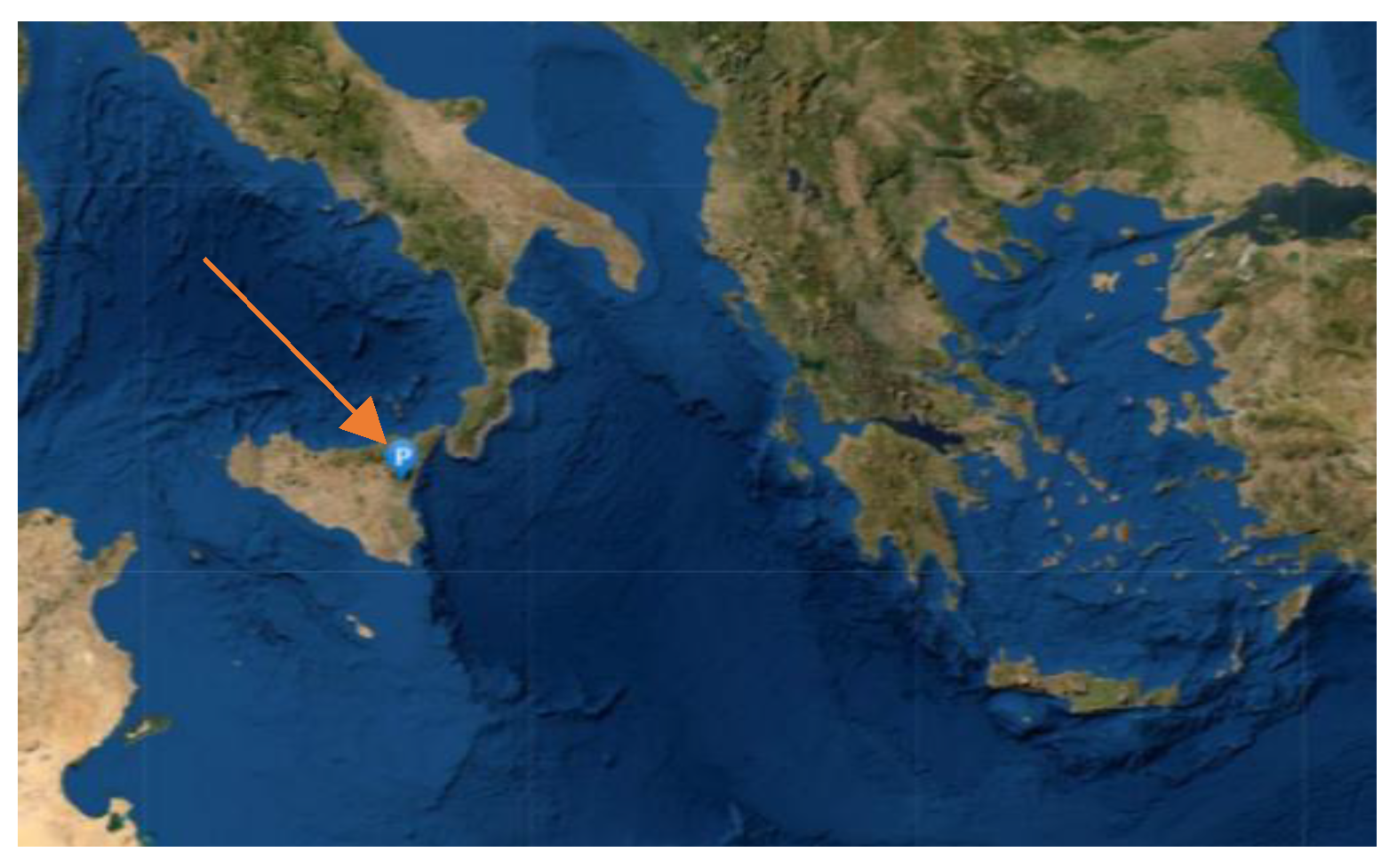
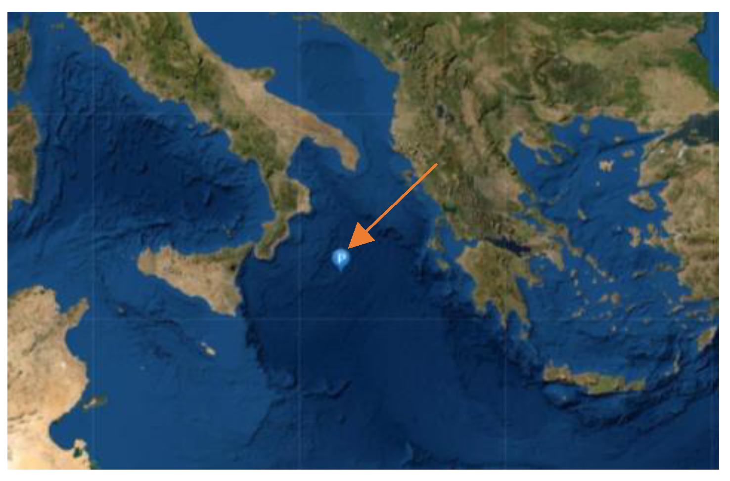
Case Study: Onshore and Offshore Sites in the Mediterranean Area

To quantify the effect of different environmental conditions on the expected useful life of PV modules in onshore and offshore environments, a hypothetical plant with the same module technology as that of the plant in [22] was considered. The environmental data that have been used in this study are from two locations in the Mediterranean area, one onshore and one offshore marine. The steps adopted to analyze the considered case study are reported in Figure 1.

The environmental data for onshore and offshore sites were imported from the NASA database [24]; it was possible to extract an hourly dataset of the environmental quantities to be used as input data of the degradation model. The resolution of these meteorological datasets is 0.5° latitude and 0.625° longitude, MERRA-2 assimilation models provide the weather parameters of the datasets. One year was chosen, from 1 January 2021 to 31 December 2021, as a sample year of data acquisition. The localizations f the two sites are reported in Figure 2 and Figure 3.

The environmental quantities extracted from the site [24] are:

• All Sky Surface Shortwave Downward Irradiance: The total solar irradiance incident (direct plus diffuse) on a horizontal plane on the surface of the Earth under all sky conditions. An alternative term for the total solar irradiance is the “global horizontal irradiance” or GHI.
• All Sky Surface UVA Irradiance: The ultraviolet A (UVA 315–400 nm) irradiance under all sky conditions.
• Temperature at 2 m: The average air (dry bulb) temperature at 2 m above the surface of the Earth.
• Relative Humidity at 2 m: The ratio of actual partial pressure of water vapor to the partial pressure at saturation, expressed in percent.
• Wind Speed at 10 m: The average wind speed at 10 m above the surface of the Earth.

Figure 4 reports a screenshot of the hourly weather dataset, downloaded from [24].

The temperature of the modules had to be calculated. The Sandia model [25] in Equation (9) was used to estimate the temperature of the modules at the considered environmental conditions; the reliability of the model is reported in [26] and further studies.

$${\mathrm{T}}_{\mathrm{mod}}={\mathrm{T}}_{\mathrm{a}}+({\mathrm{G}}_{\mathrm{POA}})·\left({\mathrm{e}}^{\mathrm{a}+\mathrm{bWs}}\right)$$

(9)

where ${\mathrm{T}}_{\mathrm{mod}}$ is the module temperature (°C), ${\mathrm{T}}_{\mathrm{a}}$ is the ambient temperature (°C), ${\mathrm{G}}_{\mathrm{POA}}$ is the front plane of array irradiance (W/${\mathrm{m}}^2$), a and b are two empirical coefficients, $\mathrm{Ws}$ is the wind speed (m/s).

The coefficients used are those suggested in [25] in the case of an open rack mounting configuration: a = −3.47, b = −0.0594.

It is possible to obtain ${\mathrm{G}}_{\mathrm{POA}}$ by using the solar angles relative to PV modules; however, in the present study, the PV modules have been hypothesized arranged on the horizontal plane in order to use the global horizontal irradiance as data input, without further processing.

The $\mathsf{\beta }$ coefficients to be used in Equation (3) should be found by calibrating the estimated degradation trend with the real degradation trend of a PV plant in similar environments.

However, due to not having historical data of PV plants in the marine environment in the present work, the estimated model coefficients in [22] are used.

Table 1. Parameter estimates of cumulative effects model along with confidence interval [22].

Parameter	Corresponding Description	Estimate	Lower 95% CI	Upper 95% CI
${\mathsf{\beta }}_0$	Frequency factor	0.35	0.21	0.50
${\mathsf{\beta }}_1$	Activation Energy	0.70	0.63	0.76
${\mathsf{\beta }}_2$	Cyclic Temperature effect	2.41	2.34	2.46
${\mathsf{\beta }}_3$	UV effect	0.75	0.68	0.89
${\mathsf{\beta }}_4$	RH effect	1.52	1.27	1.80

presents the coefficient values and confidence interval.

The initial environmental dataset is arranged in chronological order on an hourly basis within a table and can be expressed analytically as

$$\mathrm{W}\left(\mathrm{h}\right)=\left[\mathrm{GHI}\left(\mathrm{h}\right),\mathrm{UVA}\left(\mathrm{h}\right),{\mathrm{T}}_{\mathrm{a}}\left(\mathrm{h}\right),\mathrm{RH}\left(\mathrm{h}\right),\mathrm{Ws}\left(\mathrm{h}\right)\right]$$

(10)

where $\mathrm{W}\left(\mathrm{h}\right)$ is the vector representation of the data at time h, plotted in Figure A1 and Figure A2 (in Appendix A).

The data have been elaborated in order to obtain the input quantities of the model, which are on a daily basis, except the UV values, which are averaged only during the daytime.

Before applying the model, it is necessary to check all the input quantities. For this purpose, it is useful to plot them as in Figure 5 and Figure 6. It is worth noting that the T_max in these diagrams is given in °C, whereas in Sumbramaniyan’s model it must be converted to kelvin.

Usually, it would be necessary to apply filtering methods to the input quantities to exclude the non-admissible values and to replace any missing and/or incorrect data. However, using the environmental variables from the NASA database [24], it was not necessary because all the values are within the respective confidence interval.

The environmental data were consistent, with no anomalous peaks outside the admissible ranges; it was therefore possible to perform the calculations directly without the need to apply filtering methods to the acquired quantities. Starting from the acquired data, the following quantities were extrapolated: the daily data of ${\mathrm{T}}_{\max }$ and $\Delta {\mathrm{T}}_{\mathrm{daily}}$ using the temperature estimated according to the Sandia model, the average value of relative humidity (${\mathrm{RH}}_{\mathrm{daily}}$), the average value of ultraviolet irradiance (the effect of the ultraviolet A (UVA 315–400 nm) is considered) (${\mathrm{UV}}_{\mathrm{daily}}$) obtained considering exclusively the part of the day in which there is irradiation greater than 10 $\mathrm{W}/{\mathrm{m}}^2$.

The model was applied iteratively every day by extrapolating the daily contribution to the performance loss ratio; the graph shown in Figure 7 was obtained, for the onshore site.

In this way, it is assumed that every day, a combination of environmental values makes its contribution to degradation. This is not what happens physically, but it is a way to analytically represent the joint effect of environmental variables. By adding the daily degradation rate values, obtained by applying the Sumbramaniyan model, the cumulative effect is reached for the analyzed period, which in the case of this study is equal to one year.

3. Results and Discussion

To quantify the degradation of the generic PV plant, the relative variation of the power over time is defined as follows:

$$\mathrm{D}=\frac{{\mathrm{P}}_{\max }\left(\mathrm{t}\right)-{\mathrm{P}}_{\max }\left(0\right)}{{\mathrm{P}}_{\max }\left(0\right)}$$

(11)

where ${\mathrm{P}}_{\max }\left(\mathrm{t}\right)$ is the power of the PV plant at the maximum power point at time t, and ${\mathrm{P}}_{\max }\left(0\right)$ is the initial power of the PV plant at the maximum power point.

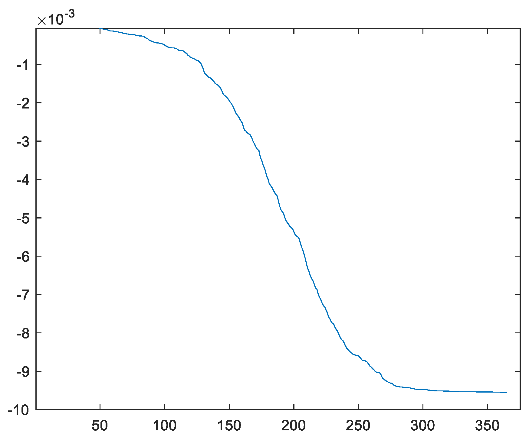
The curve in Figure 8 represent the cumulative degradation trend over a year, and the ordinate axis represents how much the maximum power has decreased compared to the maximum power that PV modules had before they came into operation for an onshore site, whereas Figure 9 and Figure 10 represent respectively the daily effect of environment on degradation trend and cumulative effect for an offshore site. The obtained values at the end of the year, equal to −0.03 and −0.0095 (−3% and −0.95%), respectively, in the onshore and offshore cases, are not reliable for many reasons:

• Even small variations in some of the used coefficients led to large variations in output. The model was calibrated under certain environmental conditions that may differ significantly from those analyzed, which could be one of the causes of the excess degradation estimated on land
• The Sumbramaniyan model was developed starting from the data of a rooftop system, so the real coefficients would be different for an open rack mounting configuration. Furthermore, the PV system on which the model is calibrated is from 1998, and the average measured degradation of the PV modules of the plant [22] is 1.3% per year in the period between 1998 and 2012, whereas current PV technologies would guarantee a lower yearly percentage degradation.
• The empirical coefficients of the Sandia thermal model used in the present work differ from those used in [22]. In the present study, the coefficients suggested in [25] were used in the case of open rack mounting.

The cumulative degradation trend, although it is not quantitatively realistic, provides useful information. It is possible to see a flattening of the curve during the coldest period, corresponding to the first and last part of the year, while the curve has a markedly greater slope during the central part of the year corresponding to the summer months.

Once the cumulative degradation curves were obtained, they were normalized with respect to the degradation value obtained at the end of the year in order to observe the different shape by overlapping the curves as in Figure 11.

Figure 11 shows that, although the degradation values obtained by the model are very different as an absolute value, the curve assumes the same trend. The cumulative exposure model shows that greater degradation occurs during the warmer months, both in offshore and onshore environments.

Comparison of Environmental Quantities and Considerations

Referring to the studies and considerations reported in the introduction, the results were unexpected: at the end of a full year of exposure to environmental conditions, a lower cumulative performance loss ratio was estimated in the case of the offshore marine site than on the onshore site.

The root cause can be found by observing the input variables of the model, statistically analyzed in the two cases in

Table 2. Statistical indices calculated for input weather data values, onshore location, 2021.

Namelist	Days	Max	Min	Mean	Median	Range	Std
${\mathrm{T}}_{\max }$	365	71.54	13.78	39.56	37.10	57.76	14.54
deltaT		45.68	4.29	26.74	27.98	41.40	9.79
${\mathrm{UV}}_{\mathrm{mean}}$		35.11	3.54	21.14	21.40	31.57	8.01
${\mathrm{UR}}_{\mathrm{mean}}$		95.48	21.40	68.19	71.65	74.08	17.43

and

Table 3. Statistical indices calculated for input weather data values, offshore location, 2021.

Namelist	Days	Max	Min	Mean	Median	Range	Std
${\mathrm{T}}_{\max }$	365	53.44	15.33	35.66	35.23	38.11	10.17
deltaT		27.23	2.19	16.22	17.31	25.04	6.39
${\mathrm{UV}}_{\mathrm{mean}}$		35.23	4.08	22.73	23.09	31.15	8.21
${\mathrm{UR}}_{\mathrm{mean}}$		97.02	57.26	76.10	75.41	39.76	8.35

.

The mean (and median) values of the daily maximum modules temperature are similar in the onshore and offshore cases. On the other hand, the mean daily temperature difference “deltaT” is about 10 °C higher in the onshore case than in the offshore case, because, in the marine environment, the temperature differences between night and day are smaller. The higher relative humidity in the marine environment affects the degradation trend; however, it does not compensate (with the coefficients used) the beneficial effect of the less extensive daily thermal cycles ($\Delta {\mathrm{T}}_{\mathrm{daily}}$).

Wind speed was taken into account through the Sandia temperature model. Wind speed is usually higher than on land, which facilitates the cooling effect exerted by convection. On the other hand, the modules will be subjected to greater mechanical stresses which, during a PV module’s useful life, could generate cell microcracks. Extreme wind events should also be considered.

A more accurate model should consider detrimental effects on photovoltaic modules generated by wind but also other environmental quantities such as waves and the sea salinity.

• Salinity

The presence of salt in the vapor sprays has harmful effects on the PV modules, and a soiling effect would be caused by the persistence of layers of salt on the modules once the water spray has evaporated. The salinity of the sea is an aspect that could be considered approximately within an analytical model. It would be useful to create plant datasets divided by technologies and climatic data (or climatic areas) in order to have data on the progress of degradation in monitored environments. This is partly achieved thanks to some studies that make the data used available; it would be possible to extend these studies to new floating onshore and offshore plants.

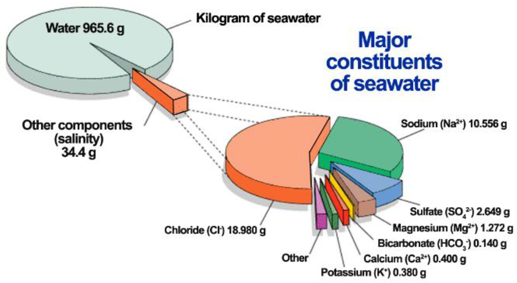
The salinity of seawater is defined as the total amount by weight of dissolved salts in one kilogram of seawater. Salinity is expressed in the unit g/kg, which is often written as ppt (part per thousand) or ‰ (per mil). Salts dissolved in seawater are dissociated into their ions; the predominant ions are chloride and sodium; other significant ions are magnesium, sulfate, calcium and potassium [27].

In [28] the constituent of 1 kg of salty water for an assigned salinity of 34.4 g/kg are graphically presented (see Figure 12).

The salinity of the sea is not uniform throughout the sea but varies, depending on the place and also over time. However, salinity, despite being uneven, is higher in coastal locations and lower further from the coast.

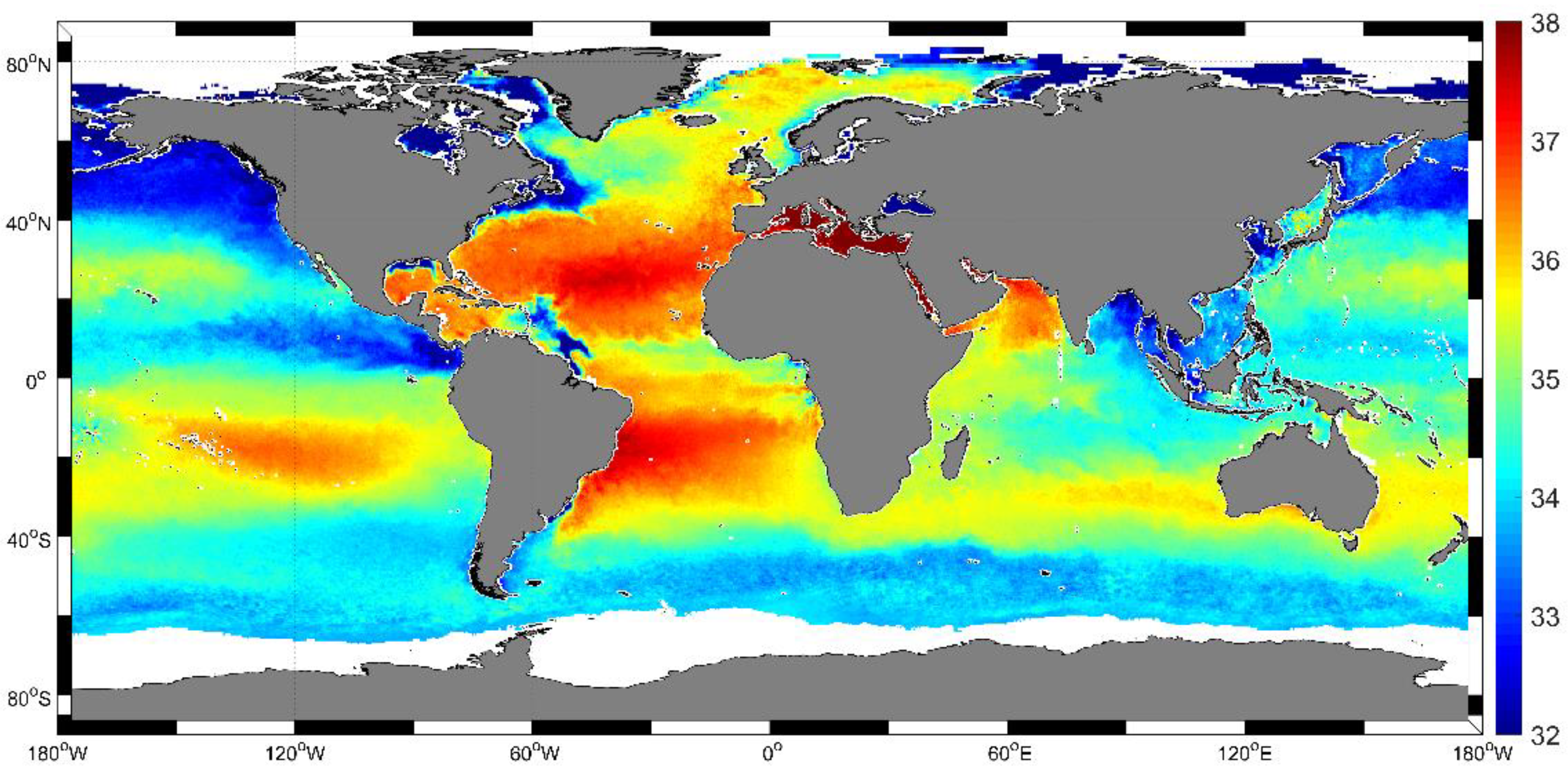
In [29] is presented a map which shows the marine salinity distribution (see Figure 13).

The dataset is based on observations from the three satellite missions that measure sea-surface salinity from space—SMOS, SMAP and Aquarius.

Sea-surface salinity is linked directly to density-driven ocean circulation patterns that transfer heat from the tropics to the poles. “Salinity is implicated in the intensification of the global water cycle. Measurements of sea-surface salinity and sea-surface temperature, which determine the thickness of the surface mixed layer, have the potential to help understand the development of extreme weather events such as cyclones [29]. Further information can be found on [https://smap.jpl.nasa.gov/ accessed on 5 January 2023].

Moreover, air–sea exchanges could be an influential parameter on the deposition of salt on the PV panels and on the degradation process, which requires a deep knowledge of the phenomena.

• Waves

One of the main challenges the modules will be subjected to is the effect of wave motion. Wave magnitude must therefore be carefully considered. The installation of floating structures in protected environments such as bays or ports can already be carried out easily with current technologies, in the presence of wave motion; on the other hand, it is necessary to carefully evaluate the most suitable types of floating structures. However, the effect of wave motion on the PV plant depends on the floating structure, so it would be complicated to take it into account in an analytical model and it would vary according to the floating structure.

The waves could affect the degradation of PVs in a mechanical way, causing vibrations due to direct impact of the waves on the floating structure or to the relative movement of its sub-components; a wavy marine environment also favors water spray and the salt deposition on the modules. Hence, the waves pose a challenge to the development of offshore PV plants. Floating structures must therefore be suitable for dealing with wave motion. Wave depends on the installation site: protected seawater surfaces will obviously be less subject to wave motion and conventional floating structures can be used; in the presence of wave motion, it is instead necessary to evaluate its impact on the PV system.

In [30], the impact of wave motion on the insulation of the PV system is evaluated. The PV modules will not remain in the pre-established tilt and orientation but will be subject to movements due to wave motion: yaw, pitch and roll movements will influence the plane-of-array irradiance hitting the modules. Simulation and an experiment are conducted. Using a moving base similar to a mini two-axis solar tracker, the effect of the wave movement is evaluated, entering the desired amplitude and period.

Pitch movements are found to be the ones that most affect production from offshore PV (up to −2.52% in the case study).

In [5], the wave motion is modeled using Fourier decomposition. In [31], a wave motion modeling is applied to a floating marine energy converter; however, the part of the modeling relating to a floating rigid body can be useful in the analysis of a generic floating structure.

The wave–structure interaction represents a fundamental aspect in the choice and design of the floating structure. In [32], a model for the simulation of the wave–structure interaction is presented where various types of both floating and submerged structures are taken into consideration. In [33], a hydroelastic investigation on a pile breakwater integrated with a flexible tail for long-wave attenuation is presented; although it is a different system from floating structures for offshore photovoltaics, the study on the “flexible tail” can be useful for photovoltaic applications as it works as a floating blanket consisting of hinged blocks, whose scale and stiffness can be easily adjusted.

4. Conclusions

In this study, the critical aspects of the degradation process related to offshore PV marine plants were presented. To estimate the difference in the degradation trend analytically, a physical data-driven model was chosen to account for the combined effect of climatic variables. The results of the model showed a lower degradation trend in the marine environment compared to that on land. This is not realistic because the environmental conditions for which the model used was calibrated are different from those analyzed in this study; moreover, no effects other than environmental input variables were considered. However, it was possible to detect a seasonal effect in the degradation process related to the combination of temperatures, thermal cycles, UV radiation and humidity characteristic of hot periods, when the estimated degradation effect is greater. To obtain more information on the degradation trend in offshore environments, it is useful to refer to specially modified indoor tests. Datasets on the degradation trend of floating offshore PV systems would be a contribution to new studies based on experimental data.