Value-Driven System Design of Utility-Scale Airborne Wind Energy

Abstract

In the current auction-based electricity market, the design of utility-scale renewable energy systems has traditionally been driven by the levelised cost of energy (LCoE). However, the market is gradually moving towards a subsidy-free era, which will expose the power plant owners to the fluctuating prices of electricity. This paper presents a computational approach to account for the influence of time-varying electricity prices on the design of airborne wind energy (AWE) systems. The framework combines an analytical performance model, providing the power curve of the system, with a wind resource characterisation based on ERA5 reanalysis data. The resulting annual energy production (AEP) model is coupled with a parametric cost model based on reference prototype data from Ampyx Power B.V. extended by scaling laws. Ultimately, an energy price model using real-life data from the ENTSO-E platform maintained by the association of EU transmission system operators was used to estimate the revenue profile. This framework was then used to compare the performance of systems based on multiple economic metrics within a chosen design space. The simulation results confirmed the expected behaviour that the electricity produced at lower wind speeds has a higher value than that produced at higher wind speeds. To account for this electricity price dependency on wind speeds in the design process, we propose an economic metric defined as the levelised profit of energy (LPoE). This approach determines the trade-offs between designing a system that minimises cost and designing a system that maximises value.

1. Introduction

Although wind energy has the highest share in the global renewable energy mix, it has far more potential than what is being harnessed today [1,2]. Airborne wind energy (AWE) is an emerging technology that uses tethered flying devices to harness the wind resource at higher altitudes (>250 m). Developers worldwide are working on different concepts, some of which are illustrated in Figure 1.

A review of the technology and the different concepts can be found in [4,5,6]. This paper was based on the widely adopted concept of converting the pulling force on the ground using a drum-generator module. For this purpose, the kite is operated in pumping cycles, alternating between the reel-out and reel-in phases. During reel-out, the kite is flown in crosswind manoeuvres to maximise the tensile power transferred to the ground and the generated electricity. For reel-in, the manoeuvres are discontinued, and the kite is flown back to the minimal tether length to start the next cycle. The reel-in phase consumes a small fraction of the generated electricity, so the net cycle power is positive. Although AWE’s research and development have accelerated over the last decade, none of the developers have been able to demonstrate the commercial viability of their technology in a relevant market. For successful diffusion of the technology in a market, the design of an AWE system should be aligned with this market’s requirements. We recognise that, at its present, relatively early stage of technology development, the industry can profit significantly from a system-level framework that captures this interaction and guides the system design to meet the market’s needs. Few studies have investigated the effect of integrating AWE systems into the energy system. Malz et al. [7] investigated the added value of AWE systems in addition to conventional wind turbines. This was performed by evaluating certain fixed system designs. The optimisation of the design to increase the value was not investigated.

System design is primarily driven by four factors: (1) the available wind resource, (2) the performance of the system, (3) the cost of the system, and (4) the value that this system creates. Performance and costs are technology-dependent, whereas wind resource and value derivation are market-dependent. It is essential to capture the influence of all four factors in a single framework.

The revenue of wind farms has long been dependent on government subsidies. As renewable energy technologies are maturing and becoming less expensive, developers now require fewer subsidies to build and operate new wind farms [8]. Since introducing competitive auctions for renewable energy technologies, subsidy-free wind power has rapidly grown in the European market [9]. In a subsidy-free future, the revenue generated by wind farms will depend on the DAM. The functioning of a typical liberalised European electricity market was described in [10,11,12]. It has been observed that the DAM prices drop when the amount of power generation through renewables in the grid increases, which is known as the merit order effect [13,14]. Accordingly, an increase in the renewable electricity supply reduces the market value of renewable electricity producers, which is known as the self-cannibalisation effect. Along with developers, the market also suffers from increasing price fluctuations. Studies such as [15,16] showed how changing the wind turbine design can help counter this effect. Turbines designed for lower specific powers (the ratio of the generator size to the rotor swept area) can produce more electricity at lower wind speeds, leading to higher earnings than turbines designed for higher specific powers. Accordingly, the wind industry is slowly evolving beyond the conventional approach of cost-driven design towards exploring various other design metrics [17,18,19]. This paper addressed this idea from the perspective of utility-scale AWE systems to reduce the gap between technology development and market introduction. We investigated if there is a shift in system design when designing for minimum cost against designing for the maximum value in the European day-ahead market (DAM) scenario. This was investigated by developing an integrated system design framework capturing the power, cost, energy, and value generation capabilities of the AWE systems.

The paper is structured as follows. Section 2 describes the system design framework and the integral models. Section 3 discusses the results using a case study. Section 4 presents the derived conclusions.

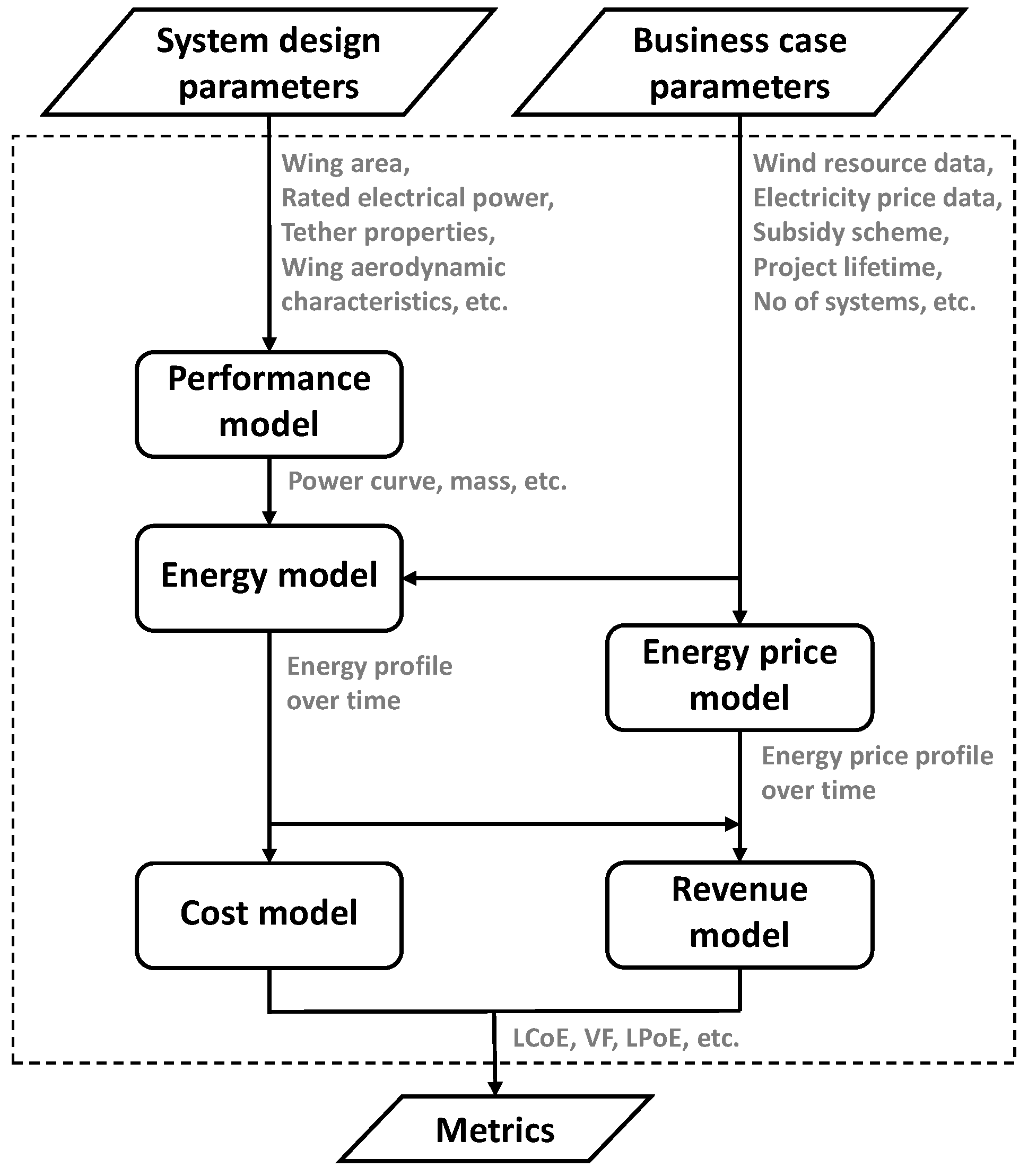
2. System Design Framework

An AWE system can be divided into three major subsystems: kite, tether, and ground station/generator. Optimising the system design is a multi-disciplinary task involving the modelling of all relevant physical interactions on the subsystem and component levels. For example, the tether force affects the structural components of the kite, consequently influencing the cost, as well as the performance of the system. However, using high-fidelity models in a design optimisation framework is computationally prohibitive and generally unnecessary for the preliminary sizing of systems.

The framework presented in this paper is based on the AWE sizing tool chain developed by Ampyx Power B.V. [20] extended with the approach described in [21]. A flowchart of this framework is shown in Figure 2. The design parameters include the properties of the kite, the tether, and the ground station/generator. The business case parameters include the wind speed data, electricity price data, project’s lifetime, number of systems, discount rate, and other financial parameters. The output includes the values of the defined metrics for each system configuration and the specified business case. A heuristic search can then find the optimal configuration with respect to the chosen metric.

The following sections describe the different model components of the framework.

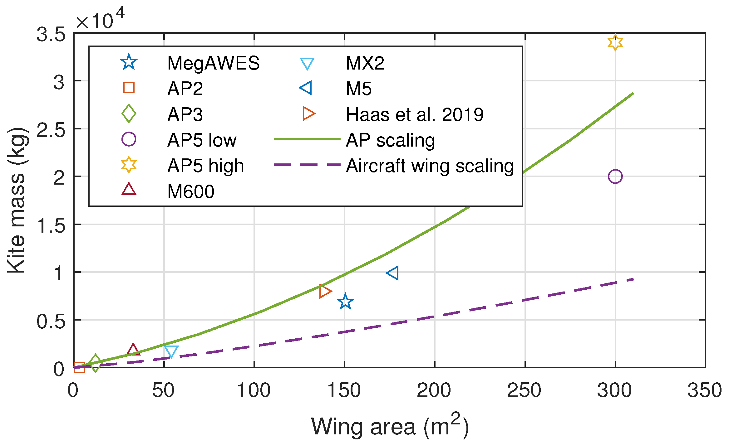
2.1. Performance Model

The performance of the AWE system was computed with an analytical model based on the steady-state aircraft dynamics introduced by Bonnin [22] for the preliminary sizing of fixed-wing AWE systems. A fast analytical model is generally preferred to a computationally expensive and more complex higher-fidelity simulation framework for such purposes. Because the analytical model uses only a limited set of input parameters, a wide range of system sizes can be investigated without generating for each case the large set of aerodynamic, control, and structural input parameters required for higher-fidelity simulations.

A basic theory for estimating the performance of AWE systems was presented by Loyd [23]. The theory considers a kite in ideal crosswind operation with the tether pointing in a downwind direction and exerting a pulling force on a drum-generator module on the ground. The mechanical power transmitted by the reeling tether is calculated as

$$P=F_t{V}_{\mathrm{w}}f,$$

(1)

where $F_t$ is the pulling force of the kite, $V_{\mathrm{w}}$ is the wind speed, and f is the tether reel-out factor defined as the ratio of reel-out speed and wind speed. Loyd derived the following expression for the pulling force.

$$F_t=\frac{1}{2}\rho V_{\mathrm{w}}^{2}S\frac{C_{\mathrm{L}}^3}{C_{\mathrm{D}}^2}{\left(1-f\right)}^2,$$

(2)

where $1/2\rho V_{\mathrm{w}}^2$ is the dynamic flow pressure, S is the wing surface area, and $C_{\mathrm{L}}^3/C_{\mathrm{D}}^2$ is the ratio of the aerodynamic coefficients. The expression illustrates that the pulling force increases quadratically with increasing wind speed, decreasing quadratically with an increasing reeling factor, and vanishing at the upper limit $f=1$. Loyd showed that the power defined by Equation (1) is maximised by an optimal reeling factor $f_{\mathrm{opt}}=1/3$. At higher wind speeds, the pulling force must be limited to the maximum allowable tether force $T_{\max }$. For this purpose, Equation (2) can be reformulated as a control law to determine the reeling factor $f>f_{\mathrm{opt}}$ as a function of $T_{\max }$. Inserting this control law into Equation (1) gives the maximum mechanical power that can be harvested at higher wind speeds:

$$P_{\max }=F_{\mathrm{t},\max }{V}_{\mathrm{W}}\left(1-\sqrt{\frac{F_{\mathrm{t},\max }}{\frac{C_{\mathrm{L}}^3}{C_{\mathrm{D}}^2}\frac{1}{2}\rho V_{\mathrm{w}}^{2}S}}\right).$$

(3)

Loyd’s theory does not account for the cyclic operation of the kite with alternating reel-out and reel-in phases. The reel-in phases and the associated power consumption are neglected, as well as effects such as the flight pattern elevation, pattern dimension, gravity, and tether sag. Luchsinger [24] extended Loyd’s theory to account for the cyclic operation with tether reel-in losses, the flight pattern elevation, and the effect of the kite mass when flying ideal circular manoeuvres around the wind vector. A similar approach was used in the present study, reducing the maximum power defined by Equation (3) by the losses from various physical effects and limitations:

• Losses due to cyclic operation with reel-in phases;
• Losses due to flight pattern elevation and dimension;
• Effective lift losses due to aircraft roll (compensating for gravity and inertia);
• Drivetrain limits (e.g., limit on maximum mechanical power);
• Design safety factors;
• Component efficiencies (i.e., gearbox, generator, power electronics etc.).

To model these physical effects, it is essential to estimate the kite and tether mass properly. For this purpose, a mass estimation model was developed using Ampyx Power’s 150 $\mathrm{kW}$ prototype as a reference system, extended by a parametric function using the wing area S, aspect ratio $AR$, and max. tether force $F_{\mathrm{t},\max }$. Figure 3 shows the kite mass as a function of the wing surface area (solid line), assuming a fixed $F_{\mathrm{t},\max }$-to-S ratio of $3.5 \mathrm{kN}/{\mathrm{m}}^2$ and a fixed-wing $AR$ of 12. The masses of several implemented and planned prototype kites were added for comparison. The aircraft wing scaling law (dashed line) is optimistic because it only includes the mass of the wing, omitting the fuselage, tail, and other electronic and electrical subsystems. The correlation provides a reference to compare the mass of conventional, untethered aircraft to that of fixed-wing kites for airborne wind energy harvesting designed for a substantially higher wing loading.

The average electrical power per cycle and the various efficiencies are defined as [31]

$$P_{\mathrm{e},\mathrm{avg}}=\frac{P_{\mathrm{RO},\mathrm{e}}{t}_{\mathrm{RO}}-P_{\mathrm{RI},\mathrm{e}}{t}_{\mathrm{RI}}}{t_{\mathrm{RO}}+t_{\mathrm{RI}}},$$

(4)

with

$$\begin{array}{c}\hfill P_{\mathrm{RO},\mathrm{e}}=P_{\mathrm{RO},\mathrm{m}}{\eta }_{\mathrm{DT}},\end{array}$$

(5)

$$\begin{array}{c}\hfill P_{\mathrm{RI},\mathrm{e}}=\frac{P_{\mathrm{RI},\mathrm{m}}}{{\eta }_{\mathrm{DT}}{\eta }_{\mathrm{Sto}}},\end{array}$$

(6)

where $P_{\mathrm{RO},\mathrm{m}}$ is the average mechanical power generated during reel-out, $t_{\mathrm{RO}}$ is the time duration of the reel-out phase, $P_{\mathrm{RI},\mathrm{m}}$ is the average mechanical power consumed during the reel-in phase, $t_{\mathrm{RI}}$ is the time duration of the reel-in phase, ${\eta }_{\mathrm{DT}}$ is the drivetrain efficiency, and ${\eta }_{\mathrm{Sto}}$ is the storage round-trip efficiency.

An AWE system can be defined with design parameters such as the wing area, aspect ratio, aerodynamic properties, tether properties, and the drivetrain properties such as the generator power limit, winch speed, acceleration, etc. For the defined system, the expression on the right-hand side of Equation (4) was maximised by numerical optimisation for every wind speed. The optimisation variables are the operational parameters such as the reel-out length, operating lift coefficient, average pattern elevation, opening cone angle of the pattern, radius of the pattern, and reel-in speed. This results in the power curve and the mass of a specified system configuration.

2.2. Energy Model

The energy production of the AWE system was computed from the output of the performance model and the available wind resource. During the cyclic operation, the kite covers a height range of approximately 200 to 400 $\mathrm{m}$. The wind speed can vary significantly due to wind shear and other atmospheric phenomena. Schelbergen et al. [32] presented an approach to compactly represent statistical wind resource data by a limited set of clustered wind profile shapes and used these for a fast estimation of the energy production of an AWE system. The method captures the variation of the wind speed with height experienced by the kite. The difference in computed energy production, assuming an average pattern height instead of the fully resolved vertical profile, was found to be insignificant. Since the framework proposed in the present paper is for preliminary sizing studies, the energy model was based on average pattern height instead of the full vertical profile. It computes the generated energy based on the wind speed distribution at the average pattern height and the power curve of the system. The annual energy production (AEP) is calculated as shown in the following equation:

$$\mathrm{AEP}=N\times 8760{\int }_{u_{\min }}^{u_{\max }}P\left(u\right)f\left(u\right)du,$$

(7)

where N is the total number of systems, u is the wind speed at the average pattern height, $P\left(u\right)$ is the power curve, and $f\left(u\right)$ is the probability of occurrence of a wind speed u.

The probability distribution of the wind speed was determined from the ERA5 reanalysis data [33]. The European Centre for Medium-Range Weather Forecasts (ECMWF) provides the dataset. It has a global coverage from 1979 to near real-time and combines model data and actual observations from around the globe within a consistent dataset. The data are provided hourly for several atmospheric, land, and sea state parameters. The surface resolution of the wind speed data in terms of latitude and longitude is ${0.25}^{\circ }$ × ${0.25}^{\circ }$, which is equivalent to around 31 $\mathrm{km}$ × 31 $\mathrm{km}$. The vertical resolution is 137 atmospheric pressure levels covering a range from 10 $\mathrm{m}$ to 80 $\mathrm{km}$. Location-specific data can be downloaded through the Copernicus Climate Change Service (C3S) Climate Data Store (CDS) [34].

The larger the dataset, the higher the accuracy of statistical models is. Therefore, for a particular location (or a business case), it is advisable to use at least five years of wind speed data with hourly resolution. It was assumed that the annual wind statistics are the same for every year, and hence, the annual energy production profile was assumed to be constant throughout the project’s lifetime. If T is the project’s lifetime, then the energy production over the project’s entire life is given by the product of T and the AEP.

2.3. Cost Model

As stated in Section 1, the four factors driving the system design of AWE are the wind resource, the system performance, the cost, and the value it creates. The first three are captured in a single economic metric known as the levelised cost of energy (LCoE). It is the average net present cost of electricity generation for a system or a plant over its entire economic lifetime, discounting costs and energy production for the time value of money [35]. The metric is calculated as

$$\mathrm{LCoE}=\frac{{\sum }_{t=0}^T\frac{\mathrm{CapEx}\left(t\right)+\mathrm{OpEx}\left(t\right)}{{(1+r)}^t}}{{\sum }_{t=0}^T\frac{E\left(t\right)}{{(1+r)}^t}},$$

(8)

where $\mathrm{CapEx}$ is the capital expenditure, $\mathrm{OpEx}$ the operational expenditure, r the discount rate, E the energy produced, and t the discrete year counter.

Due to the early stage of technology development, the literature on the cost modelling of AWE is scarce. What can be concluded is that a generalised cost model for AWE is impractical because of the diverse architectural choices in the industry. The models for soft-wing AWE systems proposed in [36,37] are mainly based on conventional wind turbine component costs translated to AWE systems. The present study was based on a cost model for a fixed-wing AWE system that was first introduced in [38]. The parametric approach was primarily based on data provided by Ampyx Power B.V. accounting for the subsystem- and component-level architectures of the specific AWE system. The cost references were based on supplier quotes, industry standards, empirical numbers, and company research [39,40,41].

Figure 4 shows the components of the cost model consisting of two modules, one for the computation of the CapEx and the other one for the computation of the OpEx. The CapEx module comprises an AWE system and balance of plant (BoP) components. The cost of the AWE system was divided into three main subsystems: (1) the kite, including the structure, electronics, and integration; (2) the tether; and (3) the ground station, which includes the drum, tether guidance mechanisms, drivetrain (including the generator, storage components, power electronics, etc.), and the launch and landing platform. The BoP is mainly relevant for the farm-level aspects and depends on the onshore, offshore, and floating business cases. The electrical infrastructure includes cabling, power electronics, grid connection, etc. Civil infrastructure includes foundations, substations, etc. Installation costs include the ports, vessels, cranes, labour costs, etc. The OpEx module comprises fixed and varying costs throughout the project’s lifetime. The fixed costs include the planned maintenance and replacement costs, and the varying costs include the unplanned failures.

Economies of scale and innovation (learning) are important for projecting the costs of innovative technologies like AWE to the point of their market entry. Learning curves can be represented by multiple cost-reducing processes such as learning by doing, researching, using, and scaling. These processes were described in [42]. There have been multiple studies [43,44,45] quantifying the learning rates of various energy technologies and their BoP costs. Different terminologies for learning factors have been used in the literature depending on the field of study. Experience/learning is generally used for cumulative production, and scale is used for size. If the cumulative production capacity or size is doubled, the specific costs reduce by a factor of $2^b$. The learning rate is defined as 1–$2^b$, and b is called the learning elasticity.

The model accounts for scale-up benefits in terms of cost per $\mathrm{k}\mathrm{W}$ of installed power. This considers the effects such as make–buy optimisation, reducing relative manpower costs, technological advancements, and others. To take these benefits into account, two learning elasticities were introduced: a for scale (size) and b for experience (cumulative production). The learning factors were applied as follows:

$$C=C_0{\left(\frac{S}{S_0}\right)}^a{\left(\frac{Q}{Q_0}\right)}^b,$$

(9)

where C is the scenario unit cost, $C_0$ is the reference unit cost, S is the scenario size, $S_0$ is the reference size, Q are the scenario units, and $Q_0$ are the reference units.

The learning elasticities can also be used per subsystem based on the known data points from the mentioned literature belonging to the relevant industry, such as conventional wind turbines, aviation, solar PV (for BoP), etc.

2.4. Electricity Price Model

As mentioned in the previous section, the only influencing factor not captured by the LCoE is the value of the generated electricity quantified by the electricity price. Traditionally, the electricity price has depended on various subsidy schemes described in [46,47]. Two of the most commonly used schemes are the feed-in-tariff (FIT) and the feed-in-premium (FIP). In an FIT scheme, the renewable energy producers are paid a fixed price per unit of electricity fed into the grid. In an FIP scheme, the producers are paid a fixed premium in addition to the day-ahead electricity market (DAM) price received per unit of electricity fed into the grid.

The DAM prices are different for different bidding zones within a country. Most European countries have one or two bidding zones with very few exceptions [48]. All power plant owners throughout the bidding zone receive the same electricity prices. The merit order effect in the DAM shows that electricity prices negatively correlate with wind power production within that zone. Based on the nature of the local wind resource, every wind farms will experience a different correlation between their production and the DAM prices. These local correlations will affect the revenue streams of the wind farm owners.

We developed the data-driven statistical model outlined in Figure 5 to verify and model the correlation between the DAM price and wind speeds. We used the wind speed time series data from the ERA5 reanalysis dataset [33] and the DAM price data from the ENTSOE-E transparency platform [49]. ENTSOE-E is responsible for collecting and publishing data related to electricity generation, transmission, and consumption in the European market.

The data preprocessing consisted of data cleaning, detrending, and removing outliers. Detrending is necessary to remove any inherent trend in the datasets to avoid spurious correlations [50]. DAM price data points three standard deviations apart were categorised as outliers. Since the wind speeds were from a modelled dataset, no data points were categorised as outliers. Temporal consistency in the datasets was maintained during these operations. The preprocessed time series datasets were then used to investigate the correlation between the variables.

The Pearson coefficient was used to evaluate the degree of correlation between wind speeds and DAM prices. The coefficient indicates the direction and strength of the linear relationship between the two statistical variables. With X being the wind speed and Y being the DAM price, the coefficient is calculated as

$$R_{\mathrm{xy}}=\frac{\mathrm{cov}(X,Y)}{\sqrt{\mathrm{var}\left(X\right)\mathrm{var}\left(Y\right)}},$$

(10)

where $\mathrm{cov}$ is the covariance and $\mathrm{var}$ is the variance of the variables.

A statistical significance test was then performed as a confirmatory test [51]. The p-value should be smaller than the chosen significance level to confirm the analysis. The commonly accepted level is 5% and, hence, was used in this model. As a next step, the ordinary least-squares method was used to model the relationship between the two variables, followed by a residual analysis to confirm the linearity of the relationship. The output of this model gave us the DAM price as a function of the wind speeds $p=f\left(u\right)$ for the specified business case. An FIT-based scenario would mean that the electricity price is independent of the wind speeds.

2.5. Revenue Model

For a subsidy-based revenue generation scenario, annual revenue can be directly estimated as the product of the AEP and electricity price. As shown in the previous section, the DAM price could be modelled as a function of the wind speeds. Therefore, for a DAM-based revenue generation scenario, annual revenue is modelled as follows:

$$\mathrm{Annual}\mathrm{revenue}=N\times 8760{\int }_{u_{\min }}^{u_{\max }}f\left(u\right)P\left(u\right)p\left(u\right)du,$$

(11)

where p is the electricity price in EUR/$\mathrm{MWh}$ and all the other variables retain their definition. The model assumes that the yearly wind statistics and the DAM price distribution are the same each year during the project’s lifetime. Therefore, the annual revenue was also assumed to be constant over the entire project’s lifetime.

Considering the time-varying electricity price scenario, there is a need for a revenue-based metric analogous to the LCoE to compare different systems based on their potential to maximise revenue. The proposed economic metric is the levelised revenue of energy (LRoE), defined as

$$\mathrm{LRoE}=\frac{{\sum }_{t=0}^T\frac{\left[p\right(t)+subsidy(t\left)\right]E\left(t\right)}{{(1+r)}^t}}{{\sum }_{t=0}^T\frac{E\left(t\right)}{{(1+r)}^t}},$$

(12)

quantifying the average net present electricity price for a project over its entire economic lifetime in EUR/$\mathrm{MWh}$. For a better comparison, the LRoE was normalised with the average market price and denoted as the value factor (VF):

$$\mathrm{VF}=\frac{\mathrm{LRoE}}{\mathrm{Average}\mathrm{DAM}\mathrm{price}}.$$

(13)

The normalised metric quantifies the difference between the average electricity price received by a producer in a time-varying electricity price scenario and the total market average price. For example, a VF of 0.8 means that the system receives 80% of the average electricity price received by its competitors in the market.

Instead of using the LCoE alone, the LCoE and LRoE should be used to compare technologies effectively. The difference between the LRoE and LCoE is defined as the levelised profit of energy (LPoE):

$$\mathrm{LPoE}=\mathrm{LRoE}-\mathrm{LCoE}.$$

(14)

To quantify the profitability of a certain investment in project planning, we define the net present value (NPV):

$$\mathrm{NPV}=\sum _{t=0}^T\frac{C_{\mathrm{t}}}{{(1+r)}^t},$$

(15)

where C is the net cash flow, i.e., the difference between the revenue and expenditure.

Since the LCoE and LRoE are both discounted to account for the time value of money, they can also be used to calculate the NPV of the project as:

$$\mathrm{NPV}=E\times \mathrm{LPoE},$$

(16)

where E is the discounted value of the total energy produced during its entire economic lifetime.

Since the LPoE and NPV capture all four factors influencing the economics of AWE, they are more comprehensive metrics to compare different design choices. In addition to the NPV, the internal rate of return (IRR) is another economic metric used to estimate the profitability of a project or an investment. The IRR is the discount rate that makes the NPV (essentially the LPoE) equal to zero. The IRR can also be used as an alternative metric to the LPoE. From the perspective of a business case, the decision for a project is generally based on a target IRR requirement of the investors. In a DAM-based scenario, it is possible that the market price alone cannot achieve this target IRR. Therefore, an additional subsidy in the form of an FIP could be necessary to achieve the required IRR.

In addition to the LCoE, these different metrics could be used to evaluate different system designs based on different objectives. The presented design framework is adaptable to evaluate different AWE concepts and business cases by modifying the necessary models and assumptions.

3. Results and Discussion

This section aims to identify system designs that can generate revenue in markets with time-varying electricity prices without the support of subsidies. This was performed by applying the presented framework to a particular case study.

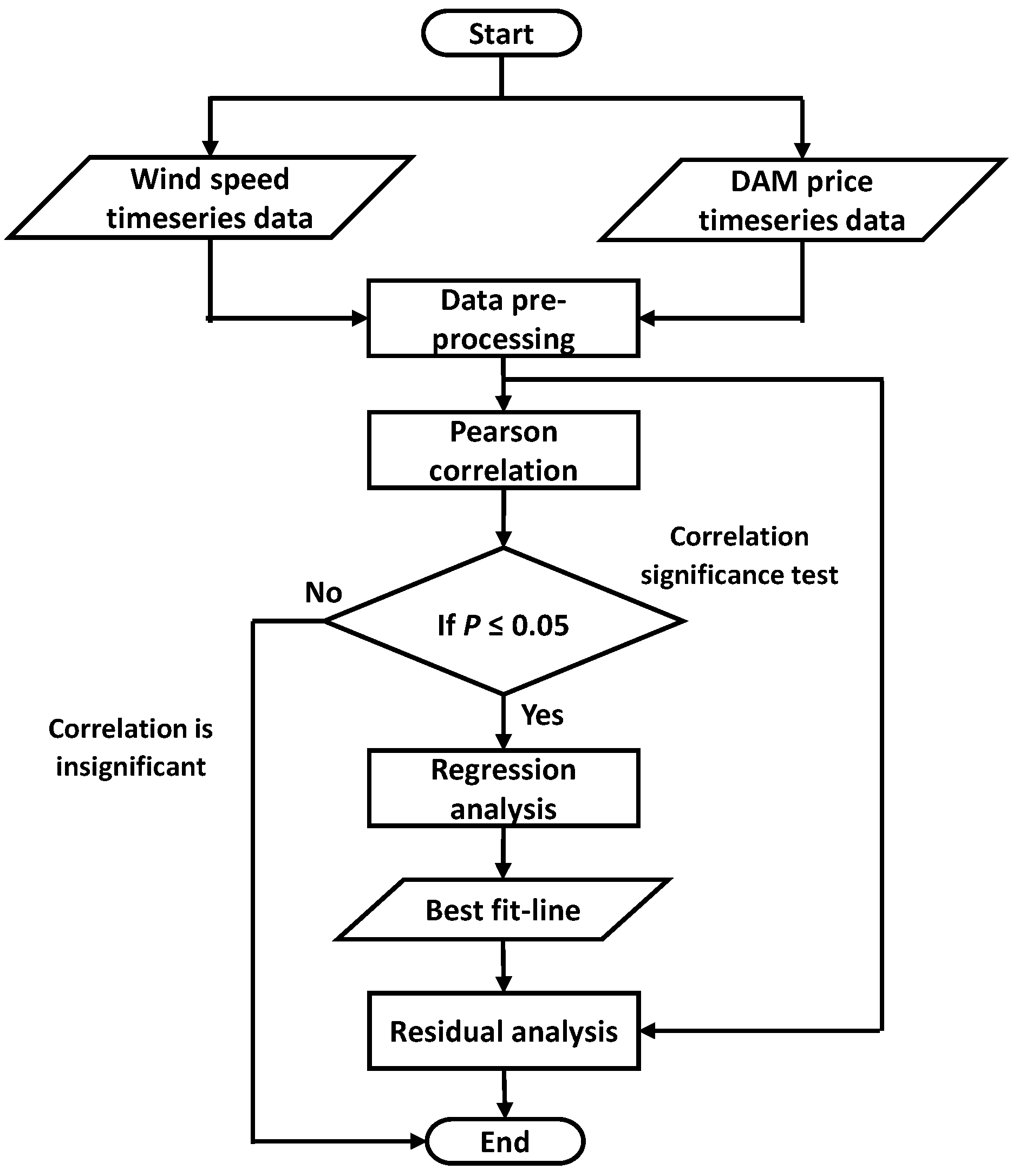
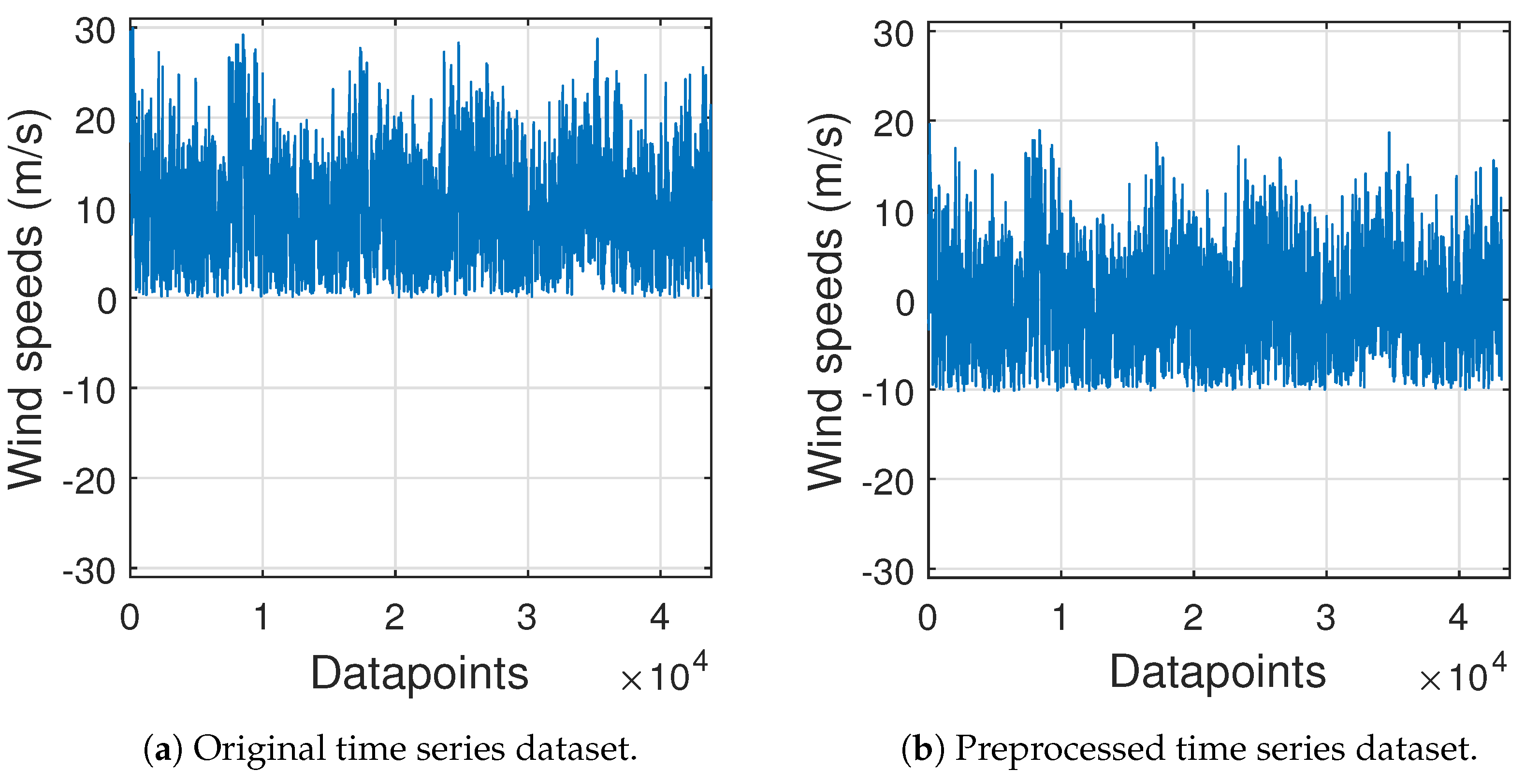
3.1. Electricity Price Dependency on Wind Speeds

An offshore location in Germany (54${}^{\circ }$N 7${}^{\circ }$E) served as an example to investigate and illustrate the dependency of the electricity price on the wind speeds. The analysis was based on a five-year historical dataset (2015 to 2019) with an hourly resolution. The height at which the wind speed data were evaluated was 350 $\mathrm{m}$. The wind speed data were obtained from [33] and the electricity price data from [49].

Figure 6 and Figure 7 show the difference between the original and the preprocessed time series of DAM prices and wind speeds, respectively. The negative wind speed values in the preprocessed data were caused by detrending the time series. The price data follow a Gaussian distribution with a mean of EUR 35/$\mathrm{MWh}$ and a standard deviation of EUR 14/$\mathrm{MWh}$. The wind speed data follow a Weibull distribution with a mean of 10 $\mathrm{m}/\mathrm{s}$. The preprocessing removed around 1.4% of the total data points.

The Pearson correlation coefficient for the dataset was $-0.33$, and the P-value was close to zero (≪0.05). This confirmed the negative correlation between wind speeds and electricity prices. The result of the regression analysis is shown in Figure 8 as the best-fit line for the data cloud. On average, an increase in wind speed by 1 $\mathrm{m}/{\mathrm{s}}^{-1}$ leads to a drop of the DAM price by EUR 0.9/$\mathrm{MWh}$.

The $R^2$ statistic of 0.11 indicates that the model did not fit the data perfectly. However, the residuals illustrated in Figure 9a,b are normally distributed with a mean of zero, which validates the linearity of the correlation because the error is spread evenly on both sides of the regression line. Therefore, the model effectively captured the required pattern within the data.

A similar analysis was performed on three locations in The Netherlands, Denmark, and Germany to check if this electricity price dependency on wind speeds can be observed in multiple European markets.

Table 1. Statistical model results: electricity price dependency on wind speeds for three different European locations.

Location	Correlation Coefficient	Slope of Regression Line
The Netherlands (52.5${}^{\circ }$ N 4.25${}^{\circ }$ E)	−0.15	−0.4
Denmark (55${}^{\circ }$ N 8${}^{\circ }$ E)	−0.38	−0.9
Germany (53${}^{\circ }$ N 12${}^{\circ }$ E)	−0.32	−1.2

shows the statistical analysis results, and all the estimated parameters were significant (i.e., p-values $\ll 0.05$).

The analysis confirmed the general trend in the European electricity markets with high wind energy penetration that electricity generated at low wind speeds has a higher value than that generated at high wind speeds.

3.2. System Sizing Case Study

Germany is one of the countries where the electricity price dependency on wind speeds has been identified to be more prominent. This results from the share of wind energy and the composition of other sources in the electricity mix. The German onshore location from Table 1 was chosen for this analysis.

Table 2. System design parameters.

Design Space Parameter	Values	Unit
Wing area	80, 120, 160, 200	${\mathrm{m}}^2$
Max. tether force	200, 300, 400, 500, 600, 700	kN
Rated power	1, 1.5, 2, 2.5	MW

and

Table 3. Business case parameters.

Business Case Parameter	Value	Unit
Avg. wind speed at 350 m	8	$\mathrm{m}/\mathrm{s}$
Avg. DAM price (2015–2019)	35	EUR/$\mathrm{MWh}$
DAM price gradient with respect to wind speed	−1.2	(EUR/$\mathrm{MWh}$)/($\mathrm{m}/{\mathrm{s}}^{-1}$)
Discount rate	10	%
Lifetime of systems	25	Years
Number of systems	30	-

list the design space and business case parameters input into the framework. The objective of the case study was to investigate if there was a shift in optimal system design when designing for different techno-economic metrics such as the LCoE, LRoE, and LPoE, as defined in the previous section.

Figure 10 depicts the power curves of four sample configurations from the design space. Figure 10a characterises a 120 m${}^2$ kite coupled to a 1.5 $\mathrm{MW}$ generator using tether force limits of 300 and 500 kN, respectively. The higher tether force limit configuration reaches the rated power earlier than the one with the lower limit. Note that the kite structure was designed to withstand the maximum force of the connected tether. Therefore, though the wing areas are the same, the kite mass for the 500 kN configuration is higher than for the 300 kN configuration. For better readability, we abbreviate the limiting value of the tether force by the term $F_{\mathrm{t},\max }$. Figure 10b characterises 80 and 160 m${}^2$ kites coupled to a 1.5 MW generator using $F_{\mathrm{t},\max }$ of 500 kN. The larger wing area configuration can produce power at lower wind speeds than the smaller one. When using the same tether material, $F_{\mathrm{t},\max }$ is directly related to the cross-sectional area of the tether, i.e., the larger the tether diameter, the higher the force limit is.

The following sections show the trends within the design space concerning the chosen metrics. The system economics heavily rely on the park size, cumulative production, and other fundamental cost assumptions. This constrained case study aimed to investigate the dependencies and not the future commercial potential of the technology. For this reason, all the presented results were normalised.

3.3. Levelised Cost of Energy Trends

Figure 11 shows the LCoE computed for all wing area and $F_{\mathrm{t},\max }$ combinations in the design space for the 2 MW generator size. We observed that each wing area was associated with a particular $F_{\mathrm{t},\max }$, which minimises the LCoE. In the case of an 80 m${}^2$ kite, the configuration with $F_{\mathrm{t},\max }$ of 400 kN achieved the minimum LCoE. This also applies to the other generator configurations in the design space.

Plotting only the optimal $F_{\mathrm{t},\max }$ configurations minimising the LCoE for each wing area revealed the LCoE trend for each generator size. This is shown in Figure 12. The derived trends can be used to identify the optimal wing area and the $F_{\mathrm{t},\max }$ configuration for specific generator sizes within the chosen business case. For each curve, the optimum configuration can be found at the minimum extreme value. The trends show that the optimal combination of the wing area and corresponding $F_{\mathrm{t},\max }$ increases with increasing generator size. The minimum extreme point for the 1 MW curve is at wing areas below 80 m${}^2$; for the 1.5 MW curve, it is at 120 m${}^2$; for the 2 MW curve, it is between 120 and 160 m${}^2$; for the 2.5 MW curve, it is at 160 m${}^2$. Above generator sizes of 2.5 MW, a 200 m${}^2$ wing area is suitable.

Several LCoE values deviated only by 5%. For developers, it is generally desirable to minimise the risk of scaling up too rapidly and to reduce the development costs. Accordingly, there can be a trade-off between lower risk (higher LCoE) and higher risk (lower LCoE). A developer could decide to use the same kite for various generator sizes. The kite has to be designed to withstand the max. tether force limit within the chosen portfolio. As an example from Figure 12, if the same $160 \mathrm{m}$ kite has to be coupled with generator sizes ranging from $1 \mathrm{MW}–2.5 \mathrm{MW}$, the kite has to be designed to withstand $F_{\mathrm{t},\max }$ of $700 \mathrm{kN}$. Hence, it will be over-designed for the $1 \mathrm{MW}$ configuration. This will affect the LCoE of the $1 \mathrm{MW}$ configuration, which needs re-evaluation.

As discussed in Section 2.3 and Section 2.4, the LCoE-driven system design does not include the effect of the time-varying electricity price. The following section shows its potential effect on system sizing.

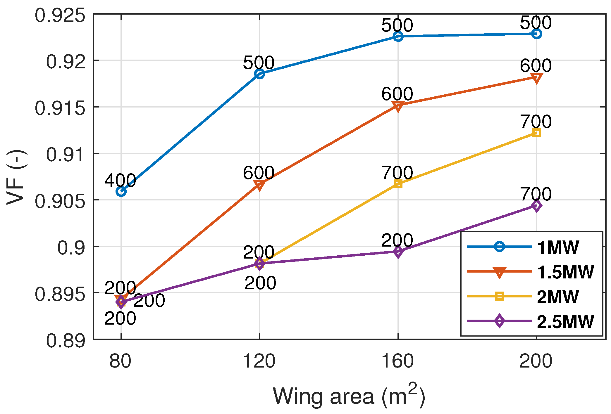
3.4. Levelised Revenue of Energy and Value Factor Trends

For the chosen business case specified in Table 3, an increase in wind speed by 1 $\mathrm{m}/{\mathrm{s}}^{-1}$ entails an average drop of the electricity price by EUR 1.2/$\mathrm{MWh}$. The effect of time-varying electricity prices on the LRoE of different system designs was assessed by calculating the value factor as defined in Equation (13). The average LRoE of all investigated designs was less than the average DAM price of EUR35/$\mathrm{MWh}$. Therefore, the value factor of all designs was less than 1, which is illustrated in Figure 13. The average value factor was around 91%, meaning that the electricity price received by the AWE systems in the market will be around 9% lower than the average electricity price received by its competitors.

The variation in the LRoE depends primarily on three aspects: the strength of the correlation between the DAM price and wind speeds, the frequency of occurrence of lower wind speeds, and the performance of the AWE system at these lower speeds. Systems with larger wing areas producing energy even at lower wind speeds are not affected as much as those with smaller wing areas with a higher cut-in wind speed.

From Figure 8, it is clear that the systems performing better at lower speeds will achieve a higher LRoE and, hence, higher value factors. From Figure 10, these are the systems with larger wing areas and higher $F_{\mathrm{t},\max }$ configurations. This suggests a trade-off between designing for low wind speeds and a system better suitable for high wind speeds, emphasising the need to shift from cost-driven system design to value-driven system design.

3.5. Levelised Profit of Energy Trends

For a subsidy-based scenario, the electricity price is independent of the wind speeds and the LRoE is identical for all system designs. Therefore, the LPoE-optimised choice will be the same as the LCoE-optimised choice. However, the same may not apply in the case of a time-varying electricity price scenario. Figure 14 shows the maximum LPoE trends for the chosen business case. The negative LPoE values mean that the LRoE of those particular system designs is lower than their LCoE. The discount rate assumption in this case study is 10%. Therefore, an LPoE of 0 corresponds to the IRR of 10%. Negative LPoE means the IRR is below the discount rate, which means that the project is not profitable with that particular configuration.

For this case study, the LRoE of all system designs was within $6\%$ of the average value. Therefore, the expected differences between LCoE-optimised and LPoE-optimised systems are not visible.

This case study was based on five years of historic data from 2015 to 2019. The electricity price and wind speed data do not show a strong negative correlation. Still, it is also not representative of the typical project lifetime of 25 years. Later years will likely exhibit a stronger correlation of wind speed and electricity price because of the increasing wind energy penetration in the European electricity market. Moreover, since the AWE system designs were not optimised, they showed a high cut-in wind speed and lower performance at lower wind speeds. These are the two main reasons that a pronounced design shift regarding the cost and value is not visible in this case study. Both factors are likely to change in future scenarios, and the value is expected to become more relevant than just the costs.

With large-scale variable renewable energy penetration, the market mechanism could also experience a change. Grid stability will have a higher value, which the LCoE does not capture. Therefore, there is an argument to optimise the systems based on drivers beyond the LCoE. Design drivers such as value, security of supply, dispatchability, and ancillary services such as frequency and voltage regulation will also become more relevant in the future.

4. Conclusions

A subsidy-free future electricity market and large-scale renewable energy penetration will expose wind farm owners to daily fluctuations in electricity prices. This will increase uncertainty in revenue generation. The merit order effect, in which the electricity prices drop with an increase in renewable electricity production, is visible in the day-ahead market. This paper provided a framework for incorporating the European electricity market’s influence on AWE system design. The aim was to evaluate if the current design trends for AWE systems are aligned with the needs that the future electricity market will likely dictate. The assessment of three locations in Germany, Denmark, and The Netherlands indicated that an increase in wind speed by 1 $\mathrm{m}/{\mathrm{s}}^{-1}$ entails an average drop of the electricity price by EUR 1/$\mathrm{MWh}$. This dependency will likely increase with the expected penetration of wind power. It was evident from the presented case study that the system having the lowest levelised cost of energy (LCoE) is not necessarily the system earning the highest revenue. For example, the $1.5 \mathrm{MW}$ system design achieved the lowest LCoE with a wing area of $120 {\mathrm{m}}^2$ and a maximum allowable tether force of $400 \mathrm{kN}$. However, for the same power rating, a system design with a wing area of $200 {\mathrm{m}}^2$ and a maximum allowable tether force of $600 \mathrm{kN}$ was able to generate the maximum revenue. It should be noted that the conclusions regarding the shift in design choices cannot be generalised because they are based on a highly specific case study. This work primarily showed the need to explore design drivers that go beyond just costs and capture the market value. The levelised profit of energy (LPoE) is one such value-based metric proposed in this paper.

References

1. Bechtle, P.; Schelbergen, M.; Schmehl, R.; Zillmann, U.; Watson, S. Airborne wind energy resource analysis. Renew. Energy 2019, 141, 1103–1116. [Google Scholar] [CrossRef]
2. Kleidon, A. Physical limits of wind energy within the atmosphere and its use as renewable energy: From the theoretical basis to practical implications. Meteorol. Z. 2021, 30, 203–225. [Google Scholar] [CrossRef]
3. Fagiano, L.; Croce, A.; Schmehl, R.; Thoms, S. (Eds.) 9th International Airborne Wind Energy Conference (AWEC 2021): Book of Abstracts; Delft University of Technology: Delft, The Netherlands, 2022. [Google Scholar] [CrossRef]
4. Vermillion, C.; Cobb, M.; Fagiano, L.; Leuthold, R.; Diehl, M.; Smith, R.S.; Wood, T.A.; Rapp, S.; Schmehl, R.; Olinger, D.; et al. Electricity in the air: Insights from two decades of advanced control research and experimental flight testing of airborne wind energy systems. Annu. Rev. Control 2021, 52, 330–357. [Google Scholar] [CrossRef]
5. Schmidt, H.; de Vries, G.; Renes, R.J.; Schmehl, R. The Social Acceptance of Airborne Wind Energy: A Literature Review. Energies 2022, 15, 1384. [Google Scholar] [CrossRef]
6. Fagiano, L.; Quack, M.; Bauer, F.; Carnel, L.; Oland, E. Autonomous Airborne Wind Energy Systems: Accomplishments and Challenges. Annu. Rev. Control. Robot. Auton. Syst. 2022, 5, 603–631. [Google Scholar] [CrossRef]
7. Malz, E.C.; Walter, V.; Göransson, L.; Gros, S. The value of airborne wind energy to the electricity system. Wind Energy 2022, 25, 281–299. [Google Scholar] [CrossRef]
8. International Renewable Energy Agency (IRENA). Renewable Power Generation Costs in 2019. Available online: https://www.irena.org/publications/2020/Jun/Renewable-Power-Costs-in-2019 (accessed on 2 January 2021).
9. International Renewable Energy Agency (IRENA). Renewable Power Remains Cost-Competitive Amid Fossil Fuel Crisis. Available online: https://www.irena.org/News/pressreleases/2022/Jul/Renewable-Power-Remains-Cost-Competitive-amid-Fossil-Fuel-Crisis (accessed on 13 January 2023).
10. Tanrisever, F.; Derinkuyu, K.; Jongen, G. Organization and functioning of liberalized electricity markets: An overview of the Dutch market. Renew. Sustain. Energy Rev. 2015, 51, 1363–1374. [Google Scholar] [CrossRef]
11. KU Leuven Energy Institute. The Current Electricity Market Design in Europe. EI Fact Sheet. 2015. Available online: https://set.kuleuven.be/ei/images/EI_factsheet8_eng.pdf (accessed on 20 November 2022).
12. Erbach, G. Understanding Electricity Markets in the EU. Briefing, European Parliamentary Research Service. 2016. Available online: https://www.europarl.europa.eu/RegData/etudes/BRIE/2016/593519/EPRS_BRI(2016)593519_EN.pdf (accessed on 20 November 2022).
13. Woo, C.K.; Horowitz, I.; Moore, J.; Pacheco, A. The impact of wind generation on the electricity spot-market price level and variance: The Texas experience. Energy Policy 2011, 39, 3939–3944. [Google Scholar] [CrossRef]
14. Hirth, L. The market value of variable renewables. The effect of solar wind power variability on their relative price. Energy Econ. 2013, 38, 218–236. [Google Scholar] [CrossRef] [Green Version]
15. Hirth, L.; Müller, S. System-friendly wind power. How advanced wind turbine design can increase the economic value of electricity generated through wind power. Energy Econ. 2016, 56, 51–63. [Google Scholar] [CrossRef]
16. Swisher, P.; Leon, J.P.M.; Gea-Bermúdez, J.; Koivisto, M.; Madsen, H.A.; Münster, M. Competitiveness of a low specific power, low cut-out wind speed wind turbine in North and Central Europe towards 2050. Appl. Energy 2022, 306, 118043. [Google Scholar] [CrossRef]
17. Garcia-Sanz, M. A Metric Space with LCOE Isolines for Research Guidance in wind and hydrokinetic energy systems. Wind Energy 2020, 23, 291–311. [Google Scholar] [CrossRef]
18. Simpson, J.; Loth, E.; Dykes, K. Cost of Valued Energy for design of renewable energy systems. Renew. Energy 2020, 153, 290–300. [Google Scholar] [CrossRef]
19. Canet, H.; Guilloré, A.; Bottasso, C.L. The eco-conscious wind turbine: Bringing societal value to design. Wind. Energy Sci. Discuss. 2022. preprint. [Google Scholar] [CrossRef]
20. Kruijff, M.; Ruiterkamp, R. A Roadmap towards Airborne Wind Energy in the Utility Sector. In Airborne Wind Energy—Advances in Technology Development and Research; Schmehl, R., Ed.; Green Energy and Technology; Springer: Singapore, 2018; Chapter 26; pp. 643–662. [Google Scholar] [CrossRef]
21. Joshi, R. Influence of the European Electricity Market on the System Design of Airborne Wind Energy. Master’s Thesis, Delft University of Technology, Delft, The Netherlands, 2020. Available online: http://resolver.tudelft.nl/uuid:a19bf3fb-9f86-4fc2-985d-d9af6481e273 (accessed on 20 November 2022).
22. Bonnin, V. An Analytical Performance Model for AP-4 Conceptual Design Phase. In Proceedings of the 8th International Airborne Wind Energy Conference (AWEC 2019): Book of Abstracts, Glasgow, UK, 15–16 October 2019; Schmehl, R., Tulloch, O., Eds.; Delft University of Technology: Delft, The Netherlands, 2019. Available online: http://resolver.tudelft.nl/uuid:e0a4471b-c11b-4c47-b409-45d62974ce94 (accessed on 20 November 2022).
23. Loyd, M.L. Crosswind kite power. J. Energy 1980, 4, 106–111. [Google Scholar] [CrossRef]
24. Luchsinger, R.H. Pumping Cycle Kite Power. In Airborne Wind Energy; Ahrens, U., Diehl, M., Schmehl, R., Eds.; Green Energy and Technology; Springer: Berlin Heidelberg, Germany, 2013; Chapter 3; pp. 47–64. [Google Scholar] [CrossRef]
25. Eijkelhof, D.; Schmehl, R. Six-degrees-of-freedom simulation model for future multi-megawatt airborne wind energy systems. Renew. Energy 2022, 196, 137–150. [Google Scholar] [CrossRef]
26. van Hagen, L. Life Cycle Assessment of Multi-Megawatt Airborne Wind Energy. Master’s Thesis, Delft University of Technology, Delft, The Netherlands, 2021. Available online: http://resolver.tudelft.nl/uuid:472a961d-1815-41f2-81b0-0c6245361efb (accessed on 20 November 2022).
27. Makani Power, INC. Response to the Federal Aviation Authority. Technical Report. 2011. Available online: http://www.energykitesystems.net/FAA/FAAfromMakani.pdf (accessed on 20 November 2022).
28. Echeverri, P.; Fricke, T.; Homsy, G.; Tucker, N. The Energy Kite: Selected Results From the Design, Development and Testing of Makani’s Airborne Wind Turbines. Technical Report. 2020. Available online: https://storage.googleapis.com/x-prod.appspot.com/files/Makani_TheEnergyKiteReport_Part1.pdf (accessed on 20 November 2022).
29. Haas, T.; Schutter, J.D.; Diehl, M.; Meyers, J. Wake characteristics of pumping mode airborne wind energy systems. J. Phys. Conf. Ser. 2019, 1256, 012016. [Google Scholar] [CrossRef] [Green Version]
30. Roskam, J. Airplane Design: Part V, Component Weight Estimation; Roskam Aviation and Engineering Corporation: Ottawa, KS, USA, 1989. [Google Scholar]
31. Fechner, U.; Schmehl, R. Model-Based Efficiency Analysis of Wind Power Conversion by a Pumping Kite Power System. In Airborne Wind Energy; Ahrens, U., Diehl, M., Schmehl, R., Eds.; Green Energy and Technology; Springer: Berlin Heidelberg, Germany, 2013. [Google Scholar] [CrossRef]
32. Schelbergen, M.; Kalverla, P.C.; Schmehl, R.; Watson, S.J. Clustering wind profile shapes to estimate airborne wind energy production. Wind Energy Sci. 2020, 5, 1097–1120. [Google Scholar] [CrossRef]
33. European Centre for Medium-Range Weather Forecasts (ECMWF). ERA5 Dataset. Available online: https://www.ecmwf.int/en/forecasts/datasets/reanalysis-datasets/era5 (accessed on 2 May 2021).
34. European Centre for Medium-Range Weather Forecasts (ECMWF). Copernicus Climate Data Store. Available online: https://cds.climate.copernicus.eu (accessed on 28 August 2020).
35. International Renewable Energy Agency (IRENA). Renewable Power Generation Costs in 2017. Available online: https://www.irena.org/publications/2018/jan/renewable-power-generation-costs-in-2017 (accessed on 4 August 2021).
36. Heilmann, J.; Houle, C. Economics of Pumping Kite Generators. In Airborne Wind Energy; Ahrens, U., Diehl, M., Schmehl, R., Eds.; Green Energy and Technology; Springer: Berlin Heidelberg, Germany, 2013; Chapter 15; pp. 271–284. [Google Scholar] [CrossRef]
37. Faggiani, P.; Schmehl, R. Design and Economics of a Pumping Kite Wind Park. In Airborne Wind Energy—Advances in Technology Development and Research; Schmehl, R., Ed.; Green Energy and Technology; Springer: Singapore, 2018; Chapter 16; pp. 391–411. [Google Scholar] [CrossRef] [Green Version]
38. Joshi, R.; Trevisi, F.; Schmehl, R.; Croce, A.; Riboldi, C. An Economic reference model for airborne wind energy systems. In Proceedings of the 9th International Airborne Wind Energy Conference (AWEC 2021): Book of Abstracts, Milano, Italy, 22–24 June 2022; Available online: http://resolver.tudelft.nl/uuid:3e9a9b47-da91-451b-b0af-2c26c7ff9612 (accessed on 20 November 2022).
39. Ampyx Power, B.V. The Sea-Air-Farm Project. Available online: https://wp.ampyxpower.com/wp-content/uploads/2020/03/Public-Summary-Final.pdf (accessed on 2 April 2021).
40. Fagan, E.M.; Engelen, S.; Bonnin, V.; Kruijff, M. Composite Production Methods for a Cost-Effective Airborne Wind Energy System. SAMPE J. 2021, 26–34. Available online: https://www.nxtbook.com/nxtbooks/sampe/journal_20210506/index.php?startid=26#/p/26 (accessed on 20 November 2022).
41. Joshi, R.; von Terzi, D.; Kruijff, M.; Schmehl, R. Techno-economic analysis of power smoothing solutions for pumping airborne wind energy systems. J. Phys. Conf. Ser. 2022. [Google Scholar] [CrossRef]
42. Wiesenthal, T.; Dowling, P.; Morbee, J.; Thiel, C.; Schade, B.; Russ, P.; Simoes, S.; Peteves, S.; Schoots, K.; Londo, M. JRC Publications Repository—Technology Learning Curves for Energy Policy Support. 2012. Available online: https://publications.jrc.ec.europa.eu/repository/handle/JRC73231 (accessed on 20 November 2022).
43. McDonald, A.; Schrattenholzer, L. Learning curves and technology assessment. Int. J. Technol. Manag. 2002, 23, 718. [Google Scholar] [CrossRef] [Green Version]
44. Rubin, E.S.; Azevedo, I.M.; Jaramillo, P.; Yeh, S. A review of learning rates for electricity supply technologies. Energy Policy 2015, 86, 198–218. [Google Scholar] [CrossRef]
45. Zhou, Y.; Gu, A. Learning curve analysis of wind power and photovoltaics technology in US: Cost reduction and the importance of research, development and demonstration. Sustainability 2019, 11, 2310. [Google Scholar] [CrossRef] [Green Version]
46. European Commission. Renewable Energy Policy Database. Available online: http://www.res-legal.eu/home/ (accessed on 2 January 2021).
47. Komusanac, I.; Fraile, D.; Brindley, G. Wind Energy in Europe in 2018—Trends and Statistics. Technical Report, Wind Europe. 2019. Available online: https://windeurope.org/wp-content/uploads/files/about-wind/statistics/WindEurope-Annual-Statistics-2018.pdf (accessed on 20 November 2022).
48. ENTSO-E. Bidding Zone Configuration Technical Report 2021. Available online: https://eepublicdownloads.azureedge.net/clean-documents/mc-documents/entso-e_bzr_technical_report_2021_211109_med.pdf (accessed on 20 November 2022).
49. European Network of Transmission System Operators for Electricity (ENTSOE-E). ENTSO-E Transparency Platform. Available online: https://transparency.entsoe.eu (accessed on 3 June 2020).
50. Raffalovich, L.E. Detrending Time Series. Sociol. Methods Res. 1994, 22, 492–519. [Google Scholar] [CrossRef]
51. Wasserman, L. All of Statistics—A Concise Course in Statistical Inference; Springer: New York, NY, USA, 2004. [Google Scholar]
Figure 1. Some of the commercial airborne wind energy concepts currently being developed [3].
Energies 16 02075 g001
Figure 2. Flowchart of the system design framework.
Energies 16 02075 g002
Figure 3. Masses of AWE systems as a function of the wing surface area. MegAWES [25], Ampyx Power AP2 and AP3 [20], AP5 low and AP5 high [26], Makani Power M600, MX2 (Oktoberkite), and M5 [27,28], Haas et al. 2019 [29], and conventional aircraft wing scaling [30].
Energies 16 02075 g003
Figure 4. Components of the cost model.
Energies 16 02075 g004
Figure 5. Flowchart of the correlation modelling method of DAM price and wind speeds.
Energies 16 02075 g005
Figure 6. Original versus preprocessed DAM price time series from Germany (2015–2019).
Energies 16 02075 g006
Figure 7. Original versus preprocessed wind speed time series from the offshore location in Germany (2015–2019).
Energies 16 02075 g007
Figure 8. Regression analysis results of the DAM prices and wind speeds from Germany (2015–2019).
Energies 16 02075 g008
Figure 9. Residuals’ analysis plots.
Energies 16 02075 g009
Figure 10. Power curves of four sample configurations from the design space listed in Table 2. (a) Effect of varying max. tether force for constant wing size.; (b) Effect of varying wing size for constant max. tether force.
Energies 16 02075 g010
Figure 11. LCoE values for the 2 MW onshore business case.
Energies 16 02075 g011
Figure 12. Minimum LCoE trend for the onshore business case. The labels at the data points quantify the F t , max in kN.
Energies 16 02075 g012
Figure 13. Maximum value factor trend for the onshore business case. The labels at the data points quantify the F t , max in kN.
Energies 16 02075 g013
Figure 14. Maximum LPoE trend for the onshore business case.
Energies 16 02075 g014