
Natural Gas Prices in the Framework of European Union’s Energy Transition: Assessing Evolution and Drivers


Abstract
:1. Introduction
- How is the evolution of European NG prices during the period 2007–2022 characterized?
- Considering NG pricing behavior, is any clustering formation identifiable?
- If there is some prevailing reasonable doubt regarding the persistence of endogeneity problems between explanatory variables and European NG prices, which kind of causality and cointegration relationships are identified?
- Which general policy recommendations can be retrieved in light of the present study?
- The general evolution of European NG prices since 2007;
- Organization of European NG prices in clusters according to years and countries;
- The confrontation between country-level household and spot market prices;
- The evolution of potential determinants of NG prices, namely:
- ⚬
- The share of energy emerging from renewable sources;
- ⚬
- The role of international trade, which includes imports and exports of NG, the share of total energy dependence, and the share of energy dependence with respect to the NG and liquefied natural gas (LNG);
- ⚬
- Supply chain elements, namely stock levels, network costs, and energy and supply costs;
- ⚬
- Components of NG prices, including direct and indirect taxation.
- In general, NG prices have remained relatively stable and without distortions caused by taxes;
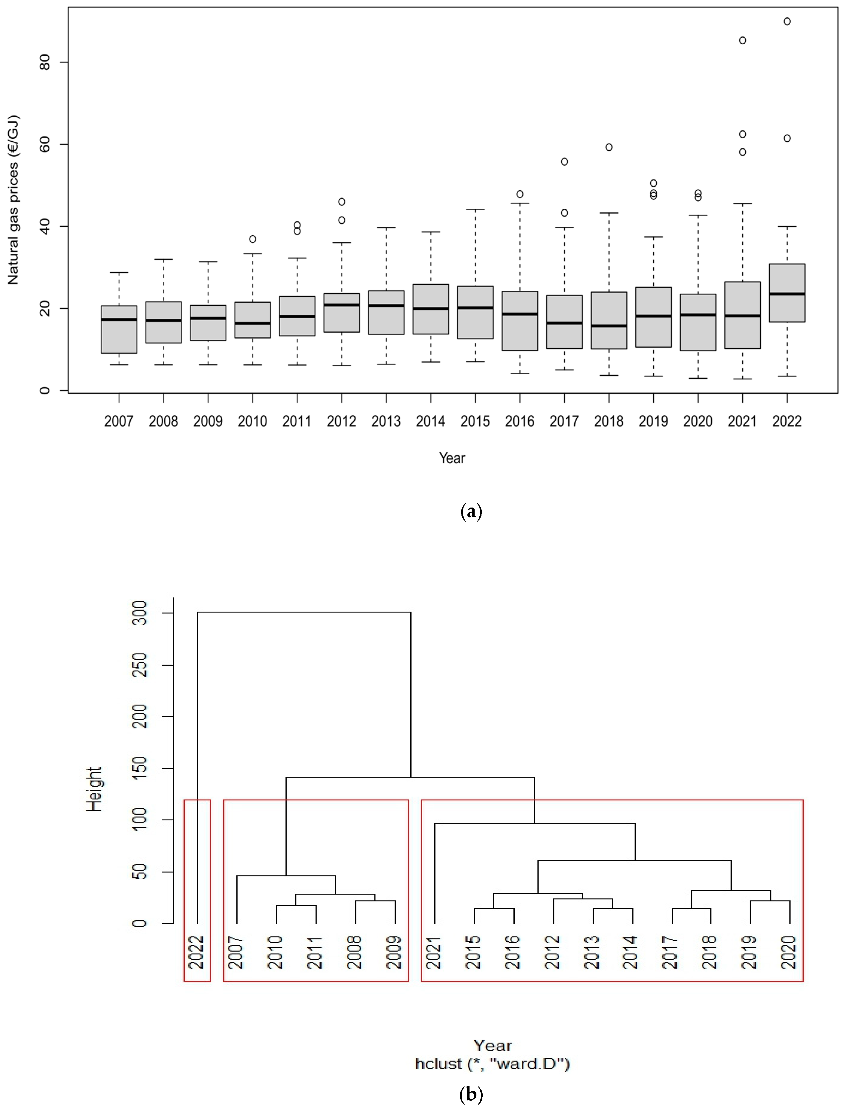
- Three distinct periods of evolution of NG prices can be identified (i.e., 2007–2011 corresponds to a period of price increases, 2012–2021 corresponds to a period of price reductions and 2022 is an outlier year characterized by galloping prices);
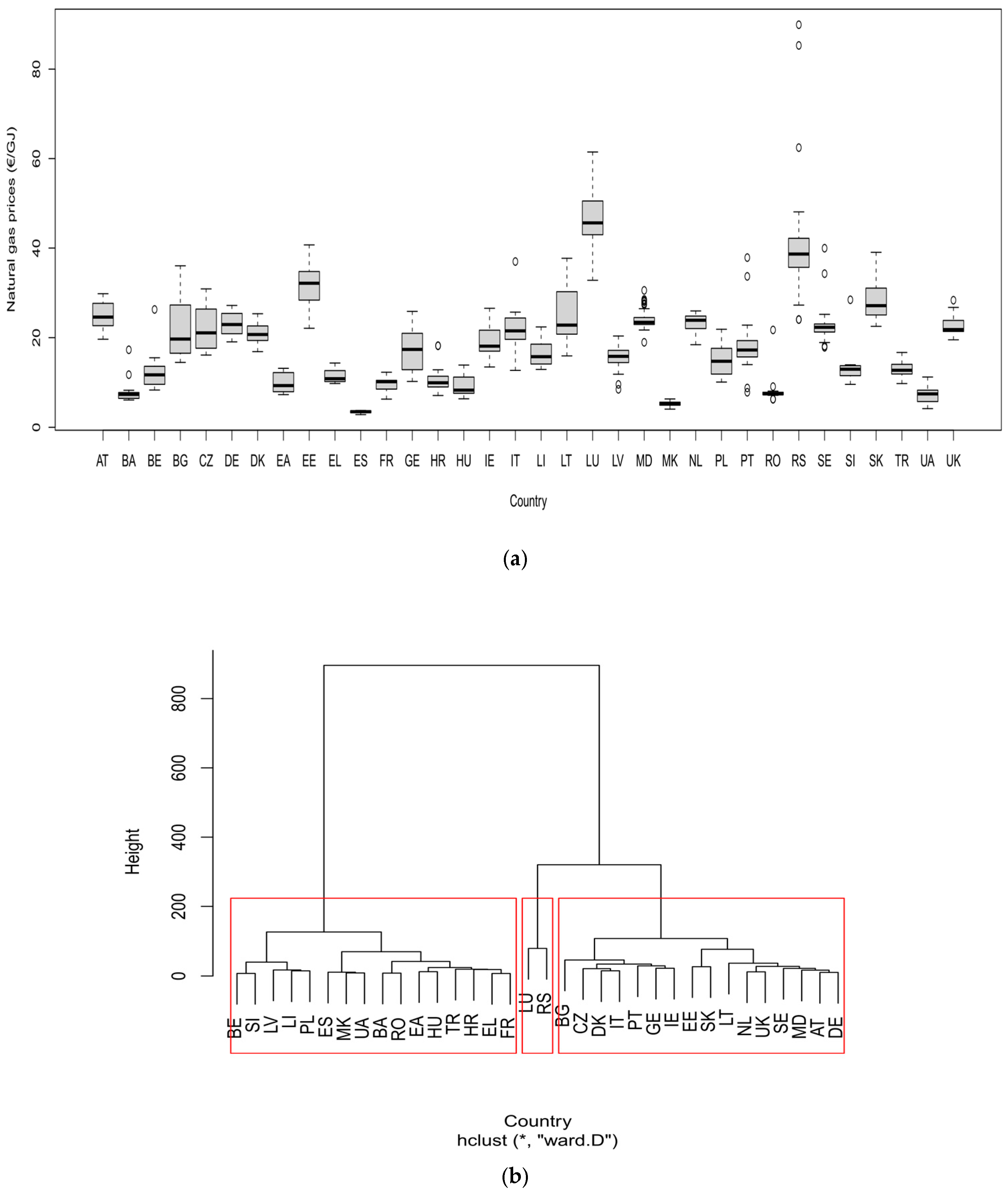
- Three distinct groups of countries are identified (i.e., the group formed by Serbia and Luxembourg exhibits the highest level of NG prices, the group formed by Bulgaria, Czechia, Denmark, Italy, Portugal, Georgia, Ireland, Estonia, Slovakia, Lithuania, Netherlands, United Kingdom, Sweden, Moldova, Austria and Germany displays intermediate NG prices and the group formed by Belgium, Slovenia, Latvia, Liechtenstein, Poland, Spain, North Macedonia, Ukraine, Bosnia and Herzegovina, Romania, Hungary, Turkey and France displays the lowest level of NG prices);
- Country-level household prices are perfectly aligned with spot market title transfer facility (TTF) prices (i.e., the parallel trends assumption holds) until the second half of 2021. From that moment on, TTF prices have increased exponentially;
- Transversely across all spatial units of the sample, the share of energy emerging from renewable sources has increased notably from 2007 to 2021;
- NG imports have remained relatively stable, eventually showing a rudimentary reduction since 2020; meanwhile, NG exports have decreased since the end of 2019. Therefore, coverage rate of imports by exports has decreased, which reflects Europe’s greater dependence on foreign countries with regard to NG;
- Within the set of European countries holding the largest stock of NG, NG prices increased from 2007 to 2021; and
- NG prices are explained by energy costs at around 35%, network costs at approximately 24% and taxation in an order of magnitude around 21%.
- Preliminary econometric tests to ensure that all classical hypotheses are satisfied, with the exception of the exogeneity of regressors in order to define a system of endogenous variables;
- A VAR-VECM model is applied to a panel data covering 34 European countries over 31 units of time corresponding to the period between 2007 and 2022 to identify if there is cointegration, causality in the sense of Granger and the direction of existing relations (e.g., unidirectional, bidirectional).
- The trend coefficient is positive but lacks statistical significance, which implies that it cannot be corroborated evidence of increasing NG prices;
- On average, the error correction term (ECT) is negative and significant, which implies evidence of cointegration between the logarithm of NG prices and LNG imports from Nigeria. Moreover, the deviation from the long run equilibrium is corrected for within the current year at a mean convergence speed of 38.304%, ceteris paribus;
- Considering a critical p-value of 1%, there is a long-run relationship between the logarithm of NG prices and LNG imports from Nigeria for approximately 30% of the 34 spatial units belonging to the sample.
- There is no bidirectional short run relationship between the variables;
- There is only a significant and unidirectional short run relation, which is imposed by LNG imports from Nigeria on the logarithm of NG prices;
- At the country level, it should be emphasized that increasing LNG imports from Nigeria has an ambiguous effect on the logarithm of NG prices; for example, NG prices are likely to increase (decrease) in Italy and Poland (the Netherlands), respectively.
2. Materials and Methods
2.1. Literature Review
- Infrastructure;
- Demand;
- Production;
- Modelling approaches.
- Liquefaction;
- Regasification;
- Shipping.
2.1.1. European Geographical and Political Context
- In some countries (e.g., The Netherlands), domestic gas reserves are decreasing significantly;
- In other countries (e.g., East Europe), new pipeline projects (e.g., the Nord Stream 2) have increased the dependence on Russia.
- Since the 2009 TEP, Europe faces strong limitations to becoming independent from Russia’s NG supply due to the establishment of long-term contract obligations;
- A long run relationship between Europe and Russia is likely to persist;
- From a medium-term perspective, the role that Russia’s NG supply will play on the European transition for a low-carbon economy must be defined;
- In the short run, solutions to transition Ukraine to the EU must be negotiated, and the scope of the regulation applied to the Turk stream must be determined.
- Eastern countries, which have a high dependence on Russia’s NG supply (>50%);
- Western countries, which have a low dependence on Russia’s NG supply (<50%).
2.1.2. NG Infrastructure
- Exploration and production (E&P);
- Transport and storage (T&S);
- Distribution;
- Consumption.
- Upstream;
- Midstream;
- Downstream.
- Southern gas corridor (SGC) in the Caspian region, which comprises non-Russian NG pipelines predominantly located in Azerbaijan and Turkmenistan [14];
- North African pipelines, including Trans-Mediterranean, Medgaz and Maghreb–Europe [17]; Emphasis should be given to Algeria’s strategic position as a gate to European NG market as long as its NG pipeline system is linked to the largest African NG source in the future, which is located in Nigeria. The Trans-Saharan NG pipeline is a 4400 km pipeline project that pretends to interconnect Nigerian NG fields with European NG markets through the Iberian Peninsula [18];
- The reservoir rock of depleted NG fields is porously and drives the need for a higher volume of cushion gas;
- Salt caverns are located underground, but they are characterized by impermeable rocks;
- Aquifers transport groundwater through porous rocks and can store NG.
2.1.3. NG Demand
- 50–60% compared to the 2010 demand with CCS; and
- 10% compared to the 2010 demand without CCS.
2.1.4. NG Production
- Synthetic NG, which stems from the use of hydrogen (H2), CO2 and biomass gasification [47];
- Green gas, which is based on renewable energy sources by considering electrolysis;
- Blue gas, which is based on NG steam methane reforming (SMR), while including CCS in the production process [48];
- Biogas, which is biomethane produced from plants and injected in NG network infrastructures [49];
- Other colored gases, such as turquoise gas (i.e., pyrolysis), pink or red (i.e., nuclear), grey (i.e., steam-methane reforming including CO2 emissions), black (i.e., hard coal), brown (i.e., lignite), orange (i.e., biogas), yellow (i.e., electricity mix) and white (i.e., H2).
2.1.5. NG Modeling Approaches
- Nonlinear optimization, simulation and heuristic (NLSH) models, which include RAMONA [53], discounted objective functions to optimize investment realization [54] and pricing [55], GASMOD [56], GASTALE [57,58,59], spatial partial equilibrium in a Hotelling city [60,61] and conjectural variation [62], GaMMES [63], EGMM [64], GGM [65], WGM [66,67], COLUMBUS [68], INGM [69], BIWGT [70], FRISBEE [71], MultiMOD through a mix complementarity problem [72], MIT EPPA [73], DYNAAMO [74], complex network theory in the form of minimum spanning tree [75] and DISCOMP [76], GEMFLOW [77,78] and a panoply of nonlinear approaches reviewed in [79], including [80,81,82,83,84,85,86,87,88].
2.1.6. LNG
- The containment system (e.g., membrane; moss type);
- The propulsion type (e.g., steam turbine; dual fuel − diesel electric),
- An increase of flexible destination contracts;
- An ongoing structural change in favor (detriment) of short-term (long-term) contracts, respectively.
2.2. Data
2.3. Nonparametric Analysis
- Firstly, we compare NG prices by the type of consumption, while considering or not the inclusion of taxes;
- Secondly, we identify similarities between NG prices between the 34 European countries (i.e., between variation), time effects in their progression (i.e., within variation) and briefly inspect the presence of seasonality effects;
- Thirdly, we confront country-level prices and TTF prices;
- Finally, we assess how the share of renewables has evolved since 2007, as well as the evolution of imports and exports of NG and LNG, energy dependence according to the type of partner, analyze stock levels and components of NG prices.
- Spearman’s correlation coefficients only describe a linear relationship between two variables rather than contemplating nonlinear relationships;
- Spearman’s correlation coefficients cannot be used to measure the association between two variables, whose distribution is given through grouped frequency tables; and
- Computations times are lengthy when the number of variable pairs is above 30.
2.4. Parametric Analysis
2.4.1. Preliminary Econometric Tests
- Specification through the Ramsey regression equation specification error test (RESET) test;
- Multicollinearity through variance inflation factor (VIF) statistics;
- Homoscedasticity through the Breusch–Pagan test;
- Absence of autocorrelation through the Breusch–Godfrey test;
- Exogeneity of regressors through the endogeneity procedure provided in [102];
2.4.2. VAR-VECM Panel Data Model Analysis
- Firstly, we analyze the cointegration between variables of interest by employing the Westerlund Error Correction Model (WECM) panel cointegration regression and respective statistical tests [105];
- Secondly, we analyze the Granger causality between the variables of interest by applying the Dumitrescu-Hurlin (DH) panel Granger causality regression and respective statistical tests [106].
- such that Equation (2) has no deterministic terms;
- such that is generated with a constant;
- such that is generated both with constant and trend.
3. Results
3.1. Nonparametric Analysis
3.1.1. NG Prices in the Segment of Households
- Band D1 represents nearly 75% of the market;
- Bands D2 and D3 have similar shares, with proportions around 12.5%.
- The first corresponds to a progressive increase of prices until 2013;
- From that moment on, prices slightly decreased until 2020;
- After 2021, prices increased exponentially.
- A first group is composed by Luxembourg and Serbia, which exhibit the highest prices;
- Countries belonging to the second group correspond to those with intermediate NG prices; this second group is composed by Bulgaria, Czechia, Denmark, Italy, Portugal, Georgia, Ireland, Estonia, Slovakia, Lithuania, Netherlands, United Kingdom, Sweden, Moldova, Austria and Germany;
- A third group comprises countries with the lowest prices, namely Belgium, Slovenia, Latvia, Liechtenstein, Poland, Spain, North Macedonia, Ukraine, Bosnia and Herzegovina, Romania, Hungary, Turkey and France.
- The COVID-19 pandemic;
- The invasion of Ukraine by Russia in February 2022.
- Regulated prices for the whole retail market in Bulgaria, France, Denmark, Greece, Hungary, Latvia, Poland and Slovakia;
- Regulated prices for the household segment in Croatia, Lithuania, Northern Ireland, Portugal, Romania and Spain;
- Two other countries (i.e., Belgium and Italy) had nonregulated prices, although with (potential) ex ante intervention in price setting. Indeed, nonregulated prices were in place only in Austria, Czech Republic, Estonia, Finland, Germany, Netherlands, Slovenia, Sweden, Republic of Ireland and UK.
3.1.2. NG Prices in the Spot Market
3.1.3. Share of Energy Emerging from Renewable Sources
3.1.4. International Trade
- Imports of NG and LNG according to the preponderance of international trade partners (Table A3, Table A4 and Table A5 in Appendix A); and
- Exports of NG according to the preponderance of international trade partners (Table A6 and Table A7 in Appendix A).
3.1.5. Energy Dependency
3.1.6. Supply
3.1.7. NG Pricing Components
- Energy and supply (NRG_SUP);
- Network costs (NETC);
- Taxes, fees, levies and charges (TAX_FEE_LEV_CHRG);
- Value added tax (VAT), renewable taxes (TAX_RNW);
- Capacity taxes (TAX_CAP);
- Environmental taxes (TAX_ENV);
- Other (OTH).
3.2. Parametric Analysis
3.2.1. Preliminary Econometric Tests
- Endogeneity tests are executed to confirm whether each explanatory variable is exogenous or not, considering the POLS model with robust standard errors. A note of mention is given to the fact that, if statistical tests detect the presence of endogeneity, then researchers need to test the orthogonality of instruments, confirm the optimal number of instruments to be added by checking whether the model should be just-identified or over-identified and test the quality of external instruments. When all the previous steps are satisfied, we apply the 2SLS/IV method to estimate coefficients. Note, however, that the goal of this study is to identify a system of endogenous variables to assess the presence of cointegration, short run relations and their direction [113,114].Following authors in [102], checking endogeneity formally requires to:
- Estimate the original structural equation, ;
- Estimate the reduce form equation for each explanatory variable to obtain residuals , which contain the endogenous information. Similar to the first step of the 2SLS/IV method, predicted values only contain the exogenous information. Hence, the potential endogenous variable is segmented into the exogenous part and the endogenous part . Formally: +; and
- Estimate the unrestricted structural equation model, whose specification includes the endogenous component in order to test the null hypothesis that the respective coefficient is null (i.e., the absence of endogenous information and, consequently, the exogeneity of ) against the alternative hypothesis capturing the presence of endogenous information and, thus, the endogeneity of .
3.2.2. VAR-VECM Panel Data Analysis
- The coefficient associated with the independent term is significant, which suggests evidence of unobserved heterogeneity affecting the nondeterministic component of the regression model;
- The trend coefficient is positive but lacks statistical significance, which implies that it cannot be corroborating evidence of increasing NG prices;
- The ECT (i.e., parameter ) associated with the regressor corresponds to the lagged value of the residuals that are obtained from the cointegration regression of the dependent variable on the set of regressors, which is derived from the long run cointegrated relationship. Hence, it determines the speed at which the system corrects back to the equilibrium relationship after a sudden shock. The result indicates that the ECT is both negative and significant. Considering the sample of 34 spatial units, this implies the prevalence of error correction such that, on average, there is evidence of cointegration between the logarithm of NG prices and LNG imports from Nigeria. Knowing that the adjustment term containing long run information is significant at the 1% level, its economic interpretation suggests that the previous year’s error—or, similarly, the deviation from the long run equilibrium—is corrected for within the current year at a mean convergence speed of 38.304%, ceteris paribus. This means that the standard compound annual growth rate (CAGR) can be applied to evaluate the number of semesters it takes for a given country to converge to the long run equilibrium. Knowing that the mathematical formula is given by , knowing that CAGR = 38.304%, EB stands for the long-term NG price target, BB stands for the short-term NG price and corresponds to the number of semesters, then a numerical exercise in which it is assumed and implies that 5 semesters (i.e., two and a half years) ensure convergence to the long run equilibrium: .
- Additionally, the 95% confidence interval of the centric coefficient that represents the ECT lies between −0.479 and −0.287, thereby implying the accommodation of a mean convergence speed ranging between 28.716% and 47.893%.
- Although the VECM regression associated with each country is not discussed in the main text for the sake of brevity, we report the estimated mean long run relationship and short run adjustment, which is given by
- No evidence in favor of a bidirectional short run relation between both variables;
- No evidence in favor of a significant and unilateral short run relation derived from the logarithm of NG prices to Nigeria’s LNG imports;
- Evidence in favor of a significant and unidirectional short run relation imposed by Nigeria’s LNG imports on NG prices.
- An increase of LNG imports from Nigeria leads to a rise of NG prices in Italy and Poland;
- An increase of LNG imports from Nigeria leads to a reduction of NG prices in the Netherlands;
- An increase of LNG imports from Nigeria implies ambiguous impact on NG prices in Portugal.
4. Discussion
4.1. Comparing the Main Results of This Study with the Existing Literature
- New competitors must be allowed to enter the LNG market;
- Existence of a vivid spot market; and
- Reduction of LNG costs.
4.2. Policy Insights and General Recommendations for Policymaking
- The decline of production and the strong dependence of NG in almost all European countries. [4];
- The increase in global temperatures has been accompanied by a growing frequency and severity of extreme weather conditions and climate disasters. In this context, the EU has already employed several measures, such as new environmental taxes to establishing renewable quotas [115]. However, although the growing of renewable energy, NG has upheld a key role in power sector [1];
- The NG demand in the near future, which is driven by incremental innovations, use of renewable energy sources and political decisions to decarbonize the energy sector. Uncertainties on these domains may deter investment realization in gas infrastructures [116].
- The liberalization of energy markets;
- The rise of global LNG trading.
- Initially, a nonparametric analysis provides useful information for policymakers, investors and managers on how European NG prices have changed. In particular, an exploratory data analysis assesses the evolution of NG prices and potential determinants affecting them from 2007 onwards where, among several stylized facts, it is confirmed that spatial units belonging to the sample are characterized by:
- ⚬
- A low level of domestic resources;
- ⚬
- A high demand for NG;
- ⚬
- A large dependence of NG from Russia, Norway and Ukraine;
- ⚬
- A large dependence of LNG from Qatar, Algeria, Nigeria, Russia and USA.
- Following that, a parametric analysis confirms that only LGN imports from Nigeria have influential power on NG prices, both in the short-term and long-term equilibria. Note that LNG, which is a green gas, holds the advantage of being strongly correlated with the increasing price trend for CO2, but also has the constraint of accommodating predominantly North African countries as predominant non-European suppliers. Indeed, the VAR-VECM panel data analysis confirms that:
- ⚬
- Increasing LNG imports from Nigeria has a significant long run impact on NG prices in approximately 30% of the sample; and
- ⚬
- Significant effects in the short run are observed in Italy, Poland and The Netherlands. Whilst the impact of increasing LNG imports from Nigeria is a price reduction in the Netherlands, a price rise holds in countries such as Italy and Poland.
- Does the one-size-fits-all logic hold when applying diversification strategies in European NG markets?
- Which costs and benefits result from applying diversification strategies in European NG markets?
- Developing new infrastructures
- Proceeding to the renewal or adaptation of existing infrastructures;
- Political adjustments for infrastructure investments and NG supply,
- Efficiency gains;
- The dissuasion of corporate practices such as price gouging and cherry-picking,
5. Conclusions
Author Contributions
Funding
Data Availability Statement
Acknowledgments
Conflicts of Interest
Appendix A. Additional Tables
Appendix A.1. General Outcomes

| Dataset | Dimension 1 | Dimension 2 | Dimension 3 |
|---|---|---|---|
| Gas prices for household consumers—bi-annual data (from 2007 onwards) Code: NRG_PC_202 Semester (1 January 2017–1 January 2022) | Type of consumption [4141901] Band D1: Consumption < 20 GJ [4141902] Band D2: 20 GJ < Consumption < 200 GJ Band D3: Consumption > 200 GJ | Taxes “I_TAX” “X_TAX” “X_VAT” | Type of unit “GJ_GCV” “KWH” |
| Gas prices for non-household consumers—bi-annual data (from 2007 onwards) Code: NRG_PC_203 Semester (1 January 2017–1 January 2022) | Type of consumption [4142901] Band I1: Consumption < 1000 GJ [4142902] Band I2: 1000 GJ < Consumption < 10,000 GJ [4142903] Band I3: 10,000 GJ < Consumption < 100,000 GJ [4142904] Band I4: 100,000 GJ < Consumption < 1,000,000 GJ [4142905] Band I5: 1,000,000 GJ < Consumption < 4,000,000 GJ [4142906] Band I6: Consumption > 4,000,000 GJ | Taxes “I_TAX” “X_TAX” “X_VAT” | Type of unit “GJ_GCV” “KWH” |
| LD Code: NRG_CB_GASM Siec: G3000 Monthly 1 January 2014→1 December 2021 | NRG_BAL [IMP] Imports [EXP] Exports [STATDIFF] Statistical | Type of unit [MIO_M3] Million cubic meters [TJ_GCV] Terajoule (gross calorific value—GCV) | |
| Household consumption volumes of gas by consumption bands Code: NRG_PC_202_V Annual (1 January 2017→1 August 2022) | Type of consumption [4141901] Band D1: Consumption < 20 GJ [4141902] Band D2: 20 GJ < Consumption < 200 GJ Band D3: Consumption > 200 GJ | Type of unit [PC] Percentage | |
| Non-household consumption volumes of gas by consumption bands Code: NRG_PC_203_V Annual (1 January 2017→1 August 2022) | Type of consumption [4142901] Band I1: Consumption < 1000 GJ [4142902] Band I2: 1000 GJ < Consumption < 10,000 GJ [4142903] Band I3: 10,000 GJ < Consumption < 100,000 GJ [4142904] Band I4: 100,000 GJ < Consumption < 1,000,000 GJ [4142905] Band I5: 1,000,000 GJ < Consumption < 4,000,000 GJ [4142906] Band I6: Consumption > 4,000,000 GJ | Type of unit [PC] Percentage | |
| Share of energy from renewable sources Code: NRG_IND_REN Annual (1 January 2004→1 August 2020) | [REN] Renewable energy sources | Type of unit [PC] Percentage | |
| Energy imports dependency Code: NRG_IND_ID] Annual (1 January 2007→1 January 2020) | Siec [TOTAL] Total [G3000] NG [O4200] NG liquids | Type of unit [PC] Percentage | |
| Imports of NG by partner country—monthly data Code: NRG_TI_GASM Monthly (1 January 2014→1 August 2022) | Siec “G3000” “G3200” | Partner (164 countries) | Type of Unit [MIO_M3] Million cubic meters [TJ_GCV] Terajoule (gross calorific value—GCV) |
| Exports of NG by partner country—monthly data Code: NRG_TE_GASM Monthly (1 January 2014→1 August 2022) | Siec “G3000” “G3200” | Partner (164 countries) | Type of Unit [MIO_M3] Million cubic meters [TJ_GCV] Terajoule (gross calorific value—GCV) |
| NG import dependency by country of origin Code NRG_IND_IDOGAS Siec: G3000 (NG) Annual (1 January 2015→1 January 2020) | “DZ” “NG” “NO” “QA” “RU” “UK” “US” | Type of unit [PC] Percentage | |
| Stock levels for gas products—monthly data Code NRG_STK_GASM Siec: G3000 Monthly (1 January 2008→1 August 2022) | stk_flow [STKCL_CG] Closing stock—cushion gas [STKOP_NAT] Opening stock—national territory [STKCL_NAT] Closing stock—national territory [STKOP_ABR] Opening stock—held abroad [STKCL_ABR] Closing stock—held abroad | Type of Unit [MIO_M3] Million cubic meters [TJ_GCV] Terajoule (gross calorific value—GCV) | |
| Gas prices components for household consumers—annual data Code: NRG_PC_202_C Annual (1 January 2017→1 January 2021) | Components of energy prices (nrg_prc) [NRG_SUP] Energy and supply [NETC] Network costs [TAX_FEE_LEV_CHRG] Taxes, fees, levies and charges on energy imports [VAT] Value added tax (VAT) [TAX_RNW] Renewable taxes [TAX_CAP] Capacity taxes [TAX_ENV] Environmental taxes | Type of consumption “4141901” “4141902” “4141903” “All.” | Type of unit “GJ_GCV” “KWH” |
| Country | MEANS | S1_2018 | S2_2018 | S1_2019 | S2_2019 | S1_2020 | S2_2020 | S1_2021 | S2_2021 | S1_2022 | DIF_21S2_20 | DIF_22_21S2 | DIF_22_20 |
|---|---|---|---|---|---|---|---|---|---|---|---|---|---|
| AT | 24.971 | 24.482 | 29.640 | 26.082 | 27.439 | 23.503 | 27.216 | 22.678 | 29.811 | NA | 26.838 | NA | NA |
| BA | 7.661 | 7.540 | 8.262 | 8.129 | 7.877 | 7.698 | 7.607 | 7.496 | 11.744 | 17.297 | 52.560 | 47.288 | 124.702 |
| BE | 12.057 | 10.877 | 11.428 | 12.076 | 12.009 | 11.716 | 11.104 | 11.637 | 14.998 | 26.292 | 28.016 | 75.301 | 124.414 |
| BG | 22.115 | 15.220 | 18.896 | 15.810 | 18.902 | 15.836 | 19.690 | 14.482 | 28.374 | 26.217 | 79.180 | −7.604 | 65.555 |
| CZ | 21.758 | 20.120 | 26.383 | 21.670 | 27.051 | 21.323 | 27.084 | 20.956 | 30.883 | 27.625 | 44.835 | −10.548 | 29.558 |
| DE | 23.185 | 22.697 | 27.083 | 24.087 | 25.209 | 21.785 | 24.892 | 20.879 | 27.192 | NA | 24.817 | NA | NA |
| DK | 20.764 | 22.617 | 24.072 | 22.314 | 23.839 | 22.632 | 23.464 | 22.497 | 24.464 | 25.345 | 8.094 | 3.602 | 11.987 |
| EA | 10.058 | 7.732 | 7.734 | 7.958 | 7.908 | 8.876 | 8.203 | 7.617 | 8.638 | 10.403 | −2.690 | 20.442 | 17.202 |
| EE | 31.491 | 33.451 | 40.703 | 36.204 | 34.111 | 31.721 | 32.715 | 29.631 | 34.762 | 33.734 | 9.586 | −2.956 | 6.347 |
| EL | 11.377 | 10.170 | 10.759 | 10.092 | 11.019 | 9.870 | 10.852 | 10.241 | 10.678 | 10.175 | 8.187 | −4.707 | 3.094 |
| ES | 3.401 | 3.679 | 3.689 | 3.740 | 3.506 | 3.427 | 2.973 | 2.831 | 3.264 | 3.501 | −4.771 | 7.290 | 2.171 |
| FR | 9.522 | 10.121 | 10.208 | 10.266 | 11.195 | 10.226 | 10.553 | 9.533 | 9.744 | 10.393 | −4.721 | 6.660 | 1.624 |
| GE | 17.504 | 16.151 | 20.974 | 18.474 | 23.968 | 19.064 | NA | NA | NA | NA | NA | NA | NA |
| HR | 10.453 | 9.091 | 10.584 | 10.635 | 10.516 | 9.477 | 8.651 | 9.004 | 18.216 | 18.179 | 92.210 | −0.207 | 91.812 |
| HU | 9.280 | 7.837 | 7.590 | 7.561 | 7.316 | 6.977 | 6.740 | 6.708 | 6.669 | 6.366 | −4.421 | −4.539 | −8.760 |
| IE | 18.926 | 16.989 | 23.034 | 17.892 | 22.283 | 18.427 | 20.673 | 17.188 | 24.583 | 23.547 | 33.408 | −4.215 | 27.784 |
| IT | 21.568 | 24.445 | 24.169 | 25.568 | 25.696 | 24.864 | 24.397 | 24.522 | 25.647 | 36.990 | 3.149 | 44.226 | 48.767 |
| LI | 16.387 | 13.771 | 13.760 | 14.119 | 13.575 | 14.824 | 13.297 | 13.369 | 14.440 | 17.199 | −2.592 | 19.105 | 16.017 |
| LT | 24.769 | 21.454 | 32.611 | 22.612 | 35.030 | 22.673 | 33.368 | 21.809 | 37.714 | 30.828 | 66.339 | −18.256 | 35.971 |
| LU | 46.542 | 32.803 | 59.288 | 37.417 | 50.518 | 47.064 | 48.065 | 58.103 | 45.553 | 61.462 | −3.211 | 34.924 | 30.592 |
| LV | 15.597 | 14.490 | 15.325 | 16.928 | 14.634 | 11.839 | 9.572 | 13.078 | 15.830 | 16.701 | 33.708 | 5.505 | 41.068 |
| MD | 24.246 | 22.627 | 24.496 | 28.024 | 28.530 | 27.365 | 28.265 | 26.469 | 27.619 | 30.554 | 0.928 | 10.627 | 11.654 |
| MK | 5.212 | 4.827 | 5.753 | 6.317 | 5.284 | 4.059 | 5.287 | 5.710 | NA | NA | NA | NA | NA |
| NL | 23.343 | 23.794 | 23.884 | 25.134 | 18.432 | 19.371 | 19.883 | 19.310 | 21.144 | NA | 9.152 | NA | NA |
| PL | 14.962 | 11.026 | 11.470 | 12.116 | 11.355 | 11.450 | 10.097 | 11.870 | 15.796 | 21.877 | 37.950 | 38.500 | 91.061 |
| PT | 18.215 | 14.530 | 16.195 | 22.593 | 22.798 | 20.443 | 22.422 | 19.343 | 33.674 | 37.867 | 64.722 | 12.451 | 85.232 |
| RO | 8.395 | 6.285 | 7.138 | 7.347 | 7.453 | 7.479 | 7.267 | 6.246 | 9.077 | 21.725 | 21.356 | 139.350 | 190.466 |
| RS | 41.389 | 38.105 | 43.257 | 48.076 | 47.451 | 42.696 | 34.698 | 62.445 | 85.298 | 89.928 | 99.777 | 5.428 | 110.621 |
| SE | 22.889 | 22.717 | 23.604 | 24.971 | 22.315 | 22.246 | 22.699 | 25.206 | 34.282 | 39.962 | 54.101 | 16.569 | 79.633 |
| SI | 13.784 | 9.581 | 12.962 | 13.944 | 13.880 | 13.073 | 10.920 | 11.702 | 13.628 | 28.452 | 4.242 | 108.779 | 117.636 |
| SK | 28.526 | 27.143 | 33.148 | 29.648 | 34.882 | 32.206 | 36.787 | 30.949 | 38.972 | 39.046 | 21.010 | 0.191 | 21.240 |
| TR | 12.938 | 12.206 | 11.898 | 11.997 | 11.977 | 11.186 | 10.601 | 9.759 | 11.168 | 16.694 | −0.169 | 49.489 | 49.237 |
| UA | 7.178 | 5.139 | 5.016 | 4.760 | 6.260 | 5.747 | 4.718 | 4.596 | 4.448 | 4.168 | −22.599 | −6.297 | −27.473 |
| UK | 22.698 | 20.940 | 22.023 | 21.034 | 21.678 | 21.757 | 21.698 | 20.965 | 21.852 | 22.852 | 0.436 | 4.576 | 5.032 |
| MEANS | 18.328 | 16.608 | 19.619 | 18.400 | 19.585 | 17.732 | 18.378 | 18.146 | 23.130 | 26.048 | 30.439 | 12.614 | 46.893 |
Appendix A.2. Monthly Imports by Partner
| Partner | IMP | IMP.Total | IMP.20-22 | IMP.Total.20–22 | Perc.IMP | Perc.IMP.20–22 |
|---|---|---|---|---|---|---|
| Total | 3395.917 | 10,636,010.710 | 3034.512 | 3,207,478.901 | 100 | 100 |
| NO | 543.662 | 1552,156.281 | 591.233 | 468,256.149 | 14.593 | 14.599 |
| RU | 426.391 | 1240,370.225 | 540.114 | 458,016.377 | 11.662 | 14.280 |
| DE | 344.376 | 982,504.994 | 334.328 | 264,787.526 | 9.238 | 8.255 |
| UA | 285.135 | 796,382.094 | 222.055 | 165,431.094 | 7.488 | 5.158 |
| SK | 234.642 | 650,427.333 | 239.623 | 173,487.333 | 6.115 | 5.409 |
| NL | 232.526 | 648,747.239 | 206.129 | 152,741.451 | 6.100 | 4.762 |
| AT | 211.324 | 592,340.143 | 212.660 | 160,558.143 | 5.569 | 5.006 |
| CZ | 180.621 | 502,487.484 | 234.987 | 172,480.484 | 4.724 | 5.377 |
| PL | 155.580 | 429,090.134 | 128.733 | 91,400.134 | 4.034 | 2.850 |
| BE | 137.993 | 389,552.873 | 155.687 | 118,322.188 | 3.663 | 3.689 |
| Country | IMP | IMP.Total | IMP.20–22 | IMP.Total.20–22 | Perc. |
|---|---|---|---|---|---|
| (a) | |||||
| DE | 2552.306 | 270,544.466 | 2916.749 | 99,169.466 | 14.279 |
| UK | 2426.708 | 198,990.061 | 1774.566 | 17,745.660 | −26.874 |
| FR | 1325.82 | 141,862.781 | 1331.565 | 46,604.781 | 0.433 |
| NL | 1309.018 | 140,064.890 | 1676.087 | 58,663.028 | 28.042 |
| BE | 1246.794 | 133,407 | 1281.706 | 44,859.700 | 2.800 |
| LT | 93.016 | 9859.700 | 115.315 | 3920.700 | 23.973 |
| ES | 55.520 | 5496.470 | 23.314 | 629.470 | −58.008 |
| DK | 22.247 | 2358.158 | 0.358 | 12.158 | −98.391 |
| TR | 15.278 | 1466.660 | 3.569 | 85.660 | −76.640 |
| (b) | |||||
| EA | 4862.142 | 481,352.039 | 6243.693 | 168,579.701 | 28.414 |
| DE | 3980.827 | 421,967.632 | 4259.342 | 144,817.632 | 6.996 |
| TR | 1344.350 | 143,845.400 | 1770.383 | 61,963.400 | 31.691 |
| BG | 952.159 | 100,928.895 | 807.556 | 27,456.895 | −15.187 |
| RS | 198.958 | 14,126 | 194.686 | 6814 | −2.147 |
| BE | 183.157 | 19,414.600 | 521.576 | 17,733.600 | 184.77 |
| NL | 138.545 | 14,685.783 | 313.200 | 10,648.783 | 126.064 |
| LV | 137.400 | 14,564.412 | 325.631 | 11,397.074 | 136.995 |
| ES | 132.633 | 14,059.118 | 117.886 | 4008.118 | −11.119 |
| UK | 83.175 | 6487.641 | 232.911 | 1397.469 | 180.025 |
| Partner | IMP | IMP.Total | IMP.20–22 | IMP.Total.20–22 | Perc.IMP | Perc.IMP.20–22 |
|---|---|---|---|---|---|---|
| TOTAL | 463.834 | 1,037,132.323 | 613.586 | 518,480.538 | 100 | 100 |
| QA | 122.426 | 346,465.513 | 129.063 | 100,410.635 | 33.406 | 19.366 |
| DZ | 83.827 | 234,714.869 | 123.038 | 92,032.631 | 22.631 | 17.750 |
| NG | 72.211 | 203,128.278 | 103.445 | 78,411.556 | 19.586 | 15.123 |
| US | 51.658 | 146,761.639 | 145.797 | 114,013.069 | 14.151 | 21.990 |
| RU | 34.347 | 97,168.493 | 96.544 | 74,242.645 | 9.369 | 14.319 |
| NO | 19.232 | 53,754.667 | 17.032 | 12,535.748 | 5.183 | 2.418 |
| TT | 14.662 | 40,687.110 | 17.721 | 12,847.533 | 3.923 | 2.478 |
| NSP | 9.327 | 25,967.505 | 4.790 | 3467.945 | 2.504 | 0.669 |
| PE | 8.377 | 23,027.462 | 2.430 | 1691.606 | 2.220 | 0.326 |
| EG | 4.273 | 11,738.384 | 12.786 | 8937.086 | 1.132 | 1.724 |
Appendix A.3. Monthly NG Exports by Partner
| Partner | EXP | EXP.Total | EXP.20–22 | EXP.Total.20–22 | Perc.EXP | P.EXP.20–22 |
|---|---|---|---|---|---|---|
| Total | 1647.659 | 4,961,102.011 | 1463.662 | 1,387,551.257 | 100 | 100 |
| DE | 367.125 | 1,034,924.642 | 378.516 | 287,293.492 | 20.861 | 20.705 |
| AT | 267.411 | 744,472.534 | 276.611 | 203,585.534 | 15.006 | 14.672 |
| CZ | 232.409 | 644,702.793 | 295.095 | 214,238.793 | 12.995 | 15.440 |
| IT | 168.841 | 472,249.427 | 172.505 | 127,480.835 | 9.519 | 9.187 |
| FR | 129.713 | 361,120.228 | 95.909 | 70,588.828 | 7.279 | 5.087 |
| BE | 127.713 | 358,489.892 | 111.192 | 82,949 | 7.226 | 5.978 |
| NL | 101.307 | 281,834.936 | 125.659 | 92,107.981 | 5.681 | 6.638 |
| CH | 69.628 | 195,586.259 | 63.946 | 48,279.165 | 3.942 | 3.479 |
| UA | 46.389 | 128,404.168 | 23.452 | 16,885.168 | 2.588 | 1.217 |
| SK | 34.884 | 96,906.959 | 57.136 | 41,708.959 | 1.953 | 3.006 |
| Partner | EXP | EXP.Total | EXP.20–22 | EXP.Total.20–22 | Perc.EXP | P.EXP.20–22 |
|---|---|---|---|---|---|---|
| Total | 25.665 | 55,281.390 | 47.924 | 36,614.052 | 100 | 100 |
| ASI_OTH | 14.988 | 11,286.200 | 13.702 | 9687.600 | 20.416 | 26.459 |
| CN | 9.438 | 7050.379 | 10.124 | 7035.907 | 12.754 | 19.216 |
| NSP | 8.083 | 22,575.737 | 2.471 | 1811.319 | 40.838 | 4.947 |
| TW | 1.939 | 1438.684 | 1.843 | 1278.900 | 2.602 | 3.493 |
| SG | 1.487 | 4073.820 | 2.445 | 1691.820 | 7.369 | 4.621 |
| KR | 1.471 | 1085.500 | 1.569 | 1085.500 | 1.964 | 2.965 |
| IN | 1.154 | 3168.990 | 2.885 | 2013.990 | 5.732 | 5.501 |
| JP | 1.104 | 3025.790 | 0.278 | 192.600 | 5.473 | 0.526 |
| BR | 1.058 | 2898.007 | 0.043 | 30.007 | 5.242 | 0.082 |
| AME_OTH | 0.944 | 696.948 | 1.007 | 696.948 | 1.261 | 1.903 |
Appendix A.4. Energy Dependency by Country of Origin
| Countries | Dep.Total | Dep.Total.20–22 | P.Dep.Total | Dep.Gas | Dep.Gas.20–22 | P.Gas | Dep.LNG | Dep.LNG.20–22 | P.LNG |
|---|---|---|---|---|---|---|---|---|---|
| AT | 64.738 | 58.324 | −9.910 | 87.921 | 73.247 | −16.690 | 23.580 | 0 | −100 |
| BA | 29.213 | 25.401 | −13.050 | 100.002 | 100 | −0.002 | 0 | 0 | -- |
| BE | 78.357 | 78.055 | −0.390 | 100.002 | 99.132 | −0.870 | 55.763 | 0 | −100 |
| BG | 40.185 | 37.882 | −5.730 | 94.420 | 96.420 | 2.118 | 0 | 0 | -- |
| CZ | 31.119 | 38.898 | 25.000 | 97.282 | 86.038 | −11.558 | 0 | 0 | -- |
| DE | 62.262 | 63.711 | 2.330 | 87.912 | 89.104 | 1.356 | 0 | 0 | -- |
| DK | 5.624 | 44.856 | 697.580 | −51.160 | 37.417 | −173.137 | 0 | 0 | -- |
| EA | -- | -- | -- | -- | -- | -- | -- | -- | -- |
| EE | 13.867 | 10.502 | −24.270 | 100 | 100 | 0 | 0 | 0 | -- |
| EL | 69.922 | 81.415 | 16.440 | 99.878 | 100.694 | 0.817 | 0 | 0 | -- |
| ES | 74.552 | 67.890 | −8.940 | 99.836 | 97.474 | −2.366 | 0 | 0 | -- |
| EU27_2020 | 56.717 | 57.497 | 1.380 | 74.655 | 83.597 | 11.978 | 90.591 | 98.705 | 8.957 |
| FR | 48.064 | 44.463 | −7.490 | 99.230 | 94.720 | −4.545 | 53.266 | 0 | −100 |
| GE | 73.537 | 79.653 | 8.320 | 99.636 | 99.671 | 0.035 | 0 | 0 | -- |
| HR | 50.234 | 53.589 | 6.680 | 33.696 | 68.774 | 104.101 | 0 | 0 | -- |
| HU | 57.475 | 56.628 | −1.470 | 82.401 | 75.622 | −8.227 | 16.201 | 0 | −100 |
| IE | 81.215 | 71.302 | −12.210 | 77.248 | 63.742 | −17.484 | 0 | 0 | -- |
| IT | 78.650 | 73.454 | −6.610 | 90.704 | 92.848 | 2.364 | 0 | 0 | -- |
| LI | -- | -- | -- | -- | -- | -- | -- | -- | -- |
| LT | 71.111 | 74.909 | 5.340 | 100.088 | 98.929 | −1.158 | 7.143 | 0 | −100 |
| LU | 96.268 | 92.458 | −3.960 | 100 | 100 | 0 | 0 | 0 | -- |
| LV | 51.148 | 45.481 | −11.080 | 96.293 | 100.099 | 3.953 | 0 | 0 | -- |
| MD | 75.648 | 75.989 | 0.450 | 99.935 | 99.544 | −0.391 | 0 | 0 | -- |
| MK | 51.566 | 63.291 | 22.740 | 100.006 | 99.992 | −0.014 | 0 | 0 | -- |
| NL | 41.911 | 68.068 | 62.410 | −39.367 | 45.032 | −214.390 | 95.849 | 104.262 | 8.777 |
| PL | 33.711 | 42.760 | 26.840 | 74.038 | 78.252 | 5.692 | 0 | 0 | -- |
| PT | 75.993 | 65.261 | −14.120 | 100.206 | 99.280 | −0.924 | 0 | 0 | -- |
| RO | 23.116 | 28.201 | 22.08 | 16.282 | 16.634 | 2.162 | −10.928 | −27.806 | 154.447 |
| RS | 31.545 | 29.836 | −5.420 | 82.196 | 79.643 | −3.106 | 30.115 | 41.867 | 39.024 |
| SE | 33.271 | 33.511 | 0.720 | 100 | 100 | 0 | 0 | 0 | -- |
| SI | 49.538 | 45.801 | −7.540 | 99.420 | 99.371 | −0.049 | 0 | 0 | -- |
| SK | 63.822 | 56.329 | −11.740 | 100.369 | 88.052 | −12.272 | 0 | 0 | -- |
| TR | 73.636 | 70.648 | −4.060 | 99.078 | 98.580 | −0.503 | 0 | 0 | -- |
| UA | 34.094 | 34.057 | −0.110 | 54.389 | 31.181 | −42.670 | 2.303 | 0 | −100 |
| UK | 35.150 | -- | -- | 42.073 | -- | -- | −9.536 | -- | -- |
| Country | DZ | NG | NO | QA | RU | UK | US | DZ.15–19 | NG.15–19 | NO.15–19 | QA.15–19 | RU.15–19 | UK.15–19 | US.15–19 |
|---|---|---|---|---|---|---|---|---|---|---|---|---|---|---|
| AL | -- | -- | -- | -- | -- | -- | -- | -- | -- | -- | -- | -- | -- | -- |
| AT | 0 | 0 | 0 | 0 | 0 | 0 | 0 | 0 | 0 | 0 | 0 | 0 | 0 | 0 |
| BA | 0 | 0 | 0 | 0 | 100 | 0 | 0 | 0 | 0 | 0 | 0 | 100 | 0 | 0 |
| BE | 0.040 | 0.210 | 50.180 | 11.960 | 14.450 | 6.640 | 3.960 | 0.112 | 0.104 | 47.116 | 12.286 | 9.260 | 6.852 | 0.422 |
| BG | 0.980 | 1.050 | 0.310 | 2.510 | 83.770 | 0 | 5.430 | 0.430 | 0.342 | 0.422 | 0.388 | 97.130 | 0 | 0.174 |
| CY | NA | NA | NA | NA | NA | NA | NA | -- | -- | -- | -- | -- | -- | -- |
| CZ | 0 | 0 | 0 | 0 | 100 | 0 | 0 | 0 | 0 | 0.360 | 0 | 99.640 | 0 | 0 |
| DE | 0 | 0.060 | 23.790 | 0.040 | 68.660 | 1.560 | 0.400 | 0.008 | 0.014 | 11.070 | 0 | 52.470 | 0.398 | 0 |
| DK | 0 | 0 | 19.580 | 0 | 62.320 | 0 | 0 | -- | -- | -- | -- | -- | -- | -- |
| EE | 0 | 0 | 1.290 | 0 | 98 | 0 | 0.710 | 0 | 0 | 0.124 | 0.006 | 99.838 | 0 | 0.006 |
| EL | 5.730 | 5.320 | 2.440 | 12.260 | 42.220 | 0.210 | 25.700 | 18.374 | 2.842 | 3.994 | 3.562 | 63.120 | 0.032 | 1.442 |
| ES | 29.610 | 12.830 | 7.290 | 8.950 | 11.520 | 0 | 15.890 | 50.164 | 12.754 | 10.618 | 9.822 | 2.940 | 0.008 | 2.932 |
| FI | 0 | 0 | 0.810 | 0 | 82.230 | 0 | 0.290 | 0 | 0 | 0.808 | 0 | 99.058 | 0.018 | 0.006 |
| FR | 8.130 | 7.590 | 38.910 | 1.770 | 19.040 | 1.040 | 2.880 | 8.568 | 5.506 | 45.182 | 3.164 | 20.354 | 1.062 | 0.784 |
| GE | 0 | 0 | 0 | 0 | 0 | 0 | 0 | 0 | 0 | 0 | 0 | 0 | 0 | 0 |
| HR | 0 | 0 | 0 | 0 | 64.110 | 0 | 0 | 0 | 0 | 0.072 | 0 | 51.288 | 0.020 | 0 |
| HU | 0 | 0 | 0 | 0 | 95 | 0 | 0 | 0 | 0 | 0 | 0 | 95 | 0 | 0 |
| IE | 0 | 0 | 0 | 0 | 0 | 100 | 0 | 0.486 | 0.148 | 35.622 | 9.090 | 1.086 | 46.876 | 0.974 |
| IS | -- | -- | -- | -- | -- | -- | -- | -- | -- | -- | -- | -- | -- | -- |
| IT | 22.840 | 0.350 | 11.880 | 10.490 | 43.720 | 0.190 | 2.720 | 23.078 | 0.168 | 5.698 | 9.286 | 46.940 | 0.306 | 0.706 |
| LI | 3 | 0 | 23.990 | 0 | 47 | 0 | 0 | 0.010 | 0.015 | 29.815 | 0.005 | 53.260 | 0.885 | 0.005 |
| LT | 0 | 0 | 37.510 | 0 | 41.790 | 0 | 20.690 | 0 | 0.752 | 42.288 | 0 | 54.914 | 0 | 2.046 |
| LU | 0.090 | 0 | 32.900 | 0 | 27.230 | 0 | 0 | 0.098 | 0 | 45.294 | 0 | 26.422 | 0 | 0 |
| LV | 0 | 0 | 0 | 0 | 100 | 0 | 0 | 0 | 0 | 0 | 0 | 100 | 0 | 0 |
| MD | 0 | 0 | 0 | 0 | 100 | 0 | 0 | 0 | 0 | 0 | 0 | 99.964 | 0 | 0 |
| ME | -- | -- | -- | -- | -- | -- | -- | -- | -- | -- | -- | -- | -- | -- |
| MK | 0 | 0 | 0 | 0 | 100 | 0 | 0 | 0 | 0 | 0 | 0 | 100 | 0 | 0 |
| MT | 0 | 0 | 0 | 0 | 0 | 0 | 18.820 | 0 | 4.730 | 1.580 | 0 | 0.107 | 0.077 | 8.770 |
| NL | 0 | 0.680 | 37.310 | 0.460 | 33.180 | 18.880 | 4.840 | 0.450 | 0.550 | 48.830 | 1 | 34.680 | 5.700 | 2.750 |
| NO | -- | -- | -- | -- | -- | -- | -- | -- | -- | -- | -- | -- | -- | -- |
| PL | 0 | 0.460 | 6.040 | 13.370 | 69.560 | 0 | 5.800 | 0 | 0 | 2.980 | 9.286 | 77.212 | 0.004 | 1.328 |
| PT | 9.340 | 53.790 | 1.370 | 2.300 | 9.700 | 0 | 18.870 | 33.912 | 33.090 | 0.718 | 9 | 0.380 | 0.026 | 8.068 |
| RO | 0 | 0 | 0 | 0 | 90.960 | 0 | 0 | 0 | 0 | 0 | 0 | 97.434 | 0 | 0 |
| RS | 0 | 0 | 0 | 0 | 100 | 0 | 0 | 0 | 0 | 0 | 0 | 100 | 0 | 0 |
| SE | 0 | 0.040 | 12.100 | 0.030 | 27.650 | 1.050 | 0.270 | 0.006 | 0.008 | 17.642 | 0.496 | 1.730 | 0.414 | 0.052 |
| SI | 0.070 | 0 | 0.030 | 0.030 | 8.820 | 0 | 0.010 | 0.076 | 0 | 0.028 | 0.054 | 26.268 | 0 | 0 |
| SK | 0 | 0 | 0 | 0 | 85.450 | 0 | 0 | 0 | 0 | 0 | 0 | 96.682 | 0 | 0 |
| TR | 11.650 | 3.950 | 0.290 | 6.770 | 33.680 | 0 | 6.220 | 9.504 | 3.884 | 0.598 | 3.998 | 48.206 | 0.032 | 1.100 |
| UA | 0.020 | 0.040 | 2.270 | 0.680 | 53.360 | 1.200 | 9.320 | 0.950 | 0.286 | 9.702 | 1.176 | 34.466 | 2.148 | 0.132 |
| UK | -- | -- | -- | -- | -- | -- | -- | 0.918 | 0.282 | 69.732 | 17.440 | 2.870 | 0.586 | 1.838 |
| Mean | 2.691 | 2.540 | 9.126 | 2.106 | 53.336 | 3.846 | 4.201 | 4.328 | 1.926 | 12.656 | 2.649 | 52.727 | 1.925 | 0.986 |
Appendix A.5. NG Pricing Components
| Country | NETC | NRG_SUP | OTH | TAX_CAP | TAX_ENV | TAX_FEE_LEV_CHRG | TAX_RNW | VAT |
|---|---|---|---|---|---|---|---|---|
| AT | 27.998 | 31.527 | 2.375 | 0 | 4.569 | 20.238 | 0 | 13.294 |
| BA | 9.992 | 64.636 | 0 | 0 | 0 | 12.686 | 0 | 12.686 |
| BE | 23.909 | 43.222 | 0.552 | 0.601 | 0.891 | 16.434 | 0.039 | 14.351 |
| BG | 22.617 | 54.689 | −4.114 | 0 | 0 | 11.347 | 0 | 15.461 |
| CZ | 14.976 | 58.984 | 0.078 | 0 | 0 | 13.020 | 0 | 12.942 |
| DE | 22.348 | 32.469 | 1.229 | 0 | 8.989 | 22.591 | 0 | 12.373 |
| DK | 14.026 | 24.522 | 0 | 0 | 16.871 | 30.726 | 0 | 13.855 |
| EA | 24.914 | 33.150 | −0.680 | 0.762 | 8.544 | 20.968 | 0.904 | 11.439 |
| EE | 10.181 | 52.036 | 0 | 0 | 5.373 | 18.891 | 0 | 13.518 |
| EL | 22.047 | 63.702 | 0.614 | 0.383 | 1.550 | 7.125 | 0 | 4.578 |
| ES | 32.666 | 30.740 | 1.053 | 1.017 | 1.849 | 18.297 | 0.200 | 14.180 |
| EU27_2020 | 24.376 | 34.323 | −0.623 | 0.697 | 8.019 | 20.650 | 0.846 | 11.712 |
| FR | 31.090 | 32.407 | 0 | 3.605 | 5.356 | 18.251 | 0 | 9.291 |
| GE | 37.372 | 36.159 | 0 | 0 | 0 | 13.235 | 0 | 13.235 |
| HR | 28.425 | 38.242 | 0 | 0 | 0 | 16.667 | 0 | 16.667 |
| HU | 20.716 | 44.211 | 0.005 | 0 | 0 | 17.536 | 0 | 17.532 |
| IE | 24.644 | 44.410 | 0 | 0 | 5.895 | 15.473 | 0 | 9.578 |
| IT | 26.242 | 41.333 | −4.804 | 0 | 9.259 | 16.212 | 1.127 | 10.630 |
| LI | 60.103 | 13.577 | 0 | 0 | 6.951 | 13.160 | 0 | 6.209 |
| LT | 37.632 | 29.526 | 0 | 1.686 | 0 | 16.421 | 0 | 14.735 |
| LU | 28.121 | 42.734 | 1.683 | 0 | 6.456 | 14.573 | 0 | 6.434 |
| LV | 46.556 | 21.623 | 0 | 0.050 | 1.267 | 15.911 | 0 | 14.594 |
| MD | 28.486 | 57.717 | 0 | 0 | 0 | 6.898 | 0 | 6.898 |
| MK | 7.771 | 65.758 | 0 | 0 | 0 | 13.235 | 0 | 13.235 |
| NL | 14.895 | 20.992 | 0 | 0 | 16.288 | 32.056 | 3.977 | 11.792 |
| PL | 22.492 | 44.552 | 0.001 | 0.002 | 0.003 | 16.478 | 0.854 | 15.618 |
| PT | 26.731 | 30.598 | 2.259 | 0 | 5.165 | 21.336 | 0 | 13.912 |
| RO | 17.283 | 55.182 | 0 | 0 | 0 | 13.768 | 0 | 13.768 |
| RS | 10.661 | 72.114 | 0.305 | 0 | 0 | 8.613 | 0 | 8.308 |
| SE | 38.937 | 17.141 | NA | NA | 6.353 | 21.961 | NA | 15.608 |
| SI | 19.716 | 35.366 | 0 | 0 | 6.194 | 22.459 | 2.281 | 13.983 |
| SK | 42.785 | 28.645 | 0 | 0 | 0 | 14.285 | 0 | 14.285 |
| TR | 14.305 | 57.582 | 0.946 | 0 | 0 | 14.056 | 0 | 13.110 |
| 2021.Mean | 25.303 | 41.026 | 0.027 | 0.275 | 3.813 | 16.835 | 0.320 | 12.419 |
| 2020.Mean | 25.454 | 40.387 | 0.309 | 0.376 | 3.725 | 17.078 | 0.379 | 12.474 |
| 2019.Mean | 24.943 | 41.584 | 0.344 | 0.346 | 3.413 | 16.737 | 0.282 | 12.351 |
| 2018.Mean | 27.092 | 42.340 | 0.581 | 0.275 | 2.955 | 17.460 | 0.145 | 13.636 |
| 2017.Mean | 27.632 | 41.557 | 0.674 | 0.267 | 2.904 | 17.741 | 0.211 | 13.830 |
Appendix B. Additional Figures
Seasonality Effects

References
- Erias, A.E.; Iglesias, E.M. Price and income elasticity of NG demand in Europe and the effects of lockdowns due to COVID-19. Energy Strategy Rev. 2022, 44, 100945. [Google Scholar] [CrossRef]
- Christie, E.H. A second life for NG demand in Europe? Energy Strategy Rev. 2012, 1, 62–65. [Google Scholar] [CrossRef]
- Grubb, M. Renewables Are Cheaper than ever—So Why Are Household Energy Bills only Going Up? The Conversation. 2022. Available online: https://theconversation.com/renewables-are-cheaper-than-ever-so-why-are-household-energy-bills-only-going-up-174795 (accessed on 1 December 2022).
- EC Quarterly Report on European Gas Markets. Market Observatory for Energy DG Energy. 2022. Available online: https://energy.ec.europa.eu/system/files/2022-04/Quarterly%20report%20on%20European%20gas%20markets_Q4%202021.pdf (accessed on 1 December 2022).
- Eurostat Eurostat Database. 2022. Available online: https://ec.europa.eu/eurostat/databrowser/explore/all/all_themes (accessed on 23 November 2022).
- De Jong, J.; Glachant, J.M.; Hafner, M.; Ahner, N.; Tagliapietra, S. A New EU Gas Security of Supply Architecture? Eur. Energy J. 2012, 2, 32–40. [Google Scholar]
- Korteweg, R. Energy as a Tool of Foreign Policy of Authoritarian States, in Particular Russia; European Parliament’s Committee on Foreign Affairs: Clingendael, The Netherlands, 2018; pp. 1–43. [Google Scholar]
- Andersen, S.S.; Sitter, N. The EU’s Strategy Towards External Gas Suppliers and Their Responses: Norway, Russia, Algeria and LNG. In New Political Economy of Energy in Europe; Godzimirski, J., Ed.; Palgrave Macmillan: Cham, Switzerland, 2018; pp. 49–72. [Google Scholar]
- EC Communication from the Commission to the European Parliament and the Council on the Short-Term Resilience of the European Gas System. Preparedness for a Possible Disruption of Supplies from the East during the Fall and Winter of 2014/2015’, (COM/2014/0654), Brussels. 2014. Available online: https://eur-lex.europa.eu/legal-content/EN/TXT/?uri=CELEX%3A52014DC0654R%2801%29 (accessed on 1 December 2022).
- EC The Role of Gas Storage in Internal Market and in Ensuring Security of Supply, Brussels. 2017. Available online: https://energy.ec.europa.eu/role-gas-storage-internal-market-and-ensuring-security-supply_en#:~:text=Depending%20on%20the%20design%20and%20characteristics%2C%20gas%20storage,the%20gas%20market%20by%20providing%20short%20term%20flexibility (accessed on 1 December 2022).
- Dickel, R.; Hassanzadeh, E.; Henderson, J.; Honoré, A.; El-Katiri, L.; Pirani, S.; Rogers, H.; Stern, J.; Yafimava, K. Reducing European Dependence on Russian Gas: Distinguishing Natural Gas Security from Geopolitics. The Oxford Institute for Energy Studies, NG92. 2014. Available online: https://www.oxfordenergy.org/wpcms/wp-content/uploads/2014/10/NG-92.pdf (accessed on 1 December 2022).
- Holz, F.; Engerer, H.; Kemfert, C.; Richter, P.M.; von Hirschhausen, C. European Natural Gas Infrastructure: The Role of Gazprom in European Natural Gas Supplies. Study Commissioned by The Greens/European Free Alliance in the European Parliament, 81; Springer: Berlin, Germany, 2014. [Google Scholar]
- GIE LNG Database. 2019. Available online: https://www.gie.eu/transparency/databases/lng-database/ (accessed on 1 December 2022).
- Sadeghi, Z.; Horry, H.R.; Khazaee, S. An economic evaluation of Iranian natural gas export to Europe through proposed pipelines. Energy Strategy Rev. 2017, 18, 1–17. [Google Scholar] [CrossRef]
- Dieckhöner, C. Simulating security of supply effects of the Nabucco and south stream projects for the European natural gas market. Energy J. 2012, 33, 153–181. [Google Scholar] [CrossRef] [Green Version]
- Chyong, C.K.; Hobbs, B.F. Strategic Eurasian natural gas market model for energy security and policy analysis: Formulation and application to South Stream. Energy Econ. 2019, 2014, 198–211. [Google Scholar] [CrossRef]
- Timmerberg, S.; Kaltschmitt, M. Hydrogen from renewables: Supply from North Africa to Central Europe as blend in existing pipelines—Potentials and costs. Appl. Energy 2019, 237, 795–809. [Google Scholar] [CrossRef]
- Odumugbo, C.A. Natural gas utilisation in Nigeria: Challenges and opportunities. J. Nat. Gas Sci. Eng. 2010, 2, 310–316. [Google Scholar] [CrossRef]
- Ruble, I. European Union energy supply security: The benefits of natural gas imports from the Eastern Mediterranean. Energy Policy 2017, 105, 341–353. [Google Scholar] [CrossRef]
- Shaffer, B. Israel-New natural gas producer in the Mediterranean. Energy Policy 2011, 39, 5379–5387. [Google Scholar] [CrossRef]
- van Oostvoorn, F. Long-Term Gas Supply Security in an Enlarged Europe. Technical Report. 2003. Available online: https://www.osti.gov/etdeweb/biblio/20464087 (accessed on 1 December 2022).
- Egging, R.; Gabriel, S.A.; Holz, F.; Zhuang, J. A complementarity model for the European natural gas market. Energy Policy 2008, 36, 2385–2414. [Google Scholar] [CrossRef] [Green Version]
- Demierre, J.; Bazilian, M.; Carbajal, J.; Sherpa, S.; Modi, V. Potential for regional use of East Africa’s natural gas. Appl. Energy 2015, 143, 414–436. [Google Scholar] [CrossRef]
- Gong, B. Effects of Ownership and Business Portfolio on Production in the Oil and Gas Industry. Energy J. 2020, 41, 33–54. [Google Scholar] [CrossRef]
- Hecking, H.; John, C.; Weiser, F. An Embargo of Russian Gas and Security of Supply in Europe. Z. Für Energ. 2015, 39, 63–73. [Google Scholar] [CrossRef]
- Woollacott, B.J.; Larson, J. Carbon-Impaired Investment: Understanding Stranded Assets in an Uncertain Energy Future. IAEE Energy Forum. 2020, pp. 47–50. Available online: https://blog.iaee.org/en/publications/newsletterdl.aspx?id=859 (accessed on 1 December 2022).
- Burandt, B.T.; Egging, R.; Assumptions, K. Stranded Assets, and the Role of Biomass and Hydrogen in the European Energy Transition. IAEE Energy Forum. 2020, pp. 33–36. Available online: https://www.iaee.org/newsletter/issue/102 (accessed on 1 December 2022).
- McKinsey Global Energy Perspective. 2021. Available online: https://www.mckinsey.com/~/media/McKinsey/Industries/Oil%20and%20Gas/Our%20Insights/Global%20Energy%20Perspective%202021/Global-Energy-Perspective-2021-final.pdf (accessed on 1 December 2022).
- Lochner, S.; Bothe, D. The development of natural gas supply costs to Europe, the United States and Japan in a globalizing gas market—Model-based analysis until 2030. Energy Policy 2009, 37, 1518–1528. [Google Scholar] [CrossRef]
- Hall, M. Norwegian Gas Exports: Assessment of Resources and Supply to 2035’, Oxford Institute for Energy Studies, NG127. 2018. Available online: https://www.oxfordenergy.org/wpcms/wp-content/uploads/2018/03/Norwegian-Gas-Exports-Assessment-of-Resources-and-Supply-to-2035-NG-127.pdf (accessed on 1 December 2022).
- ENTSO-G Ten-Year Network Development Plan 2017. Brussels. 2017. Available online: https://www.entsog.eu/sites/default/files/entsog-migration/publications/TYNDP/2017/entsog_tyndp_2017_main_170428_web_xs.pdf (accessed on 1 December 2022).
- Eser, P.; Chokani, N.; Abhari, R. Impact of Nord Stream 2 and LNG on gas trade and security of supply in the European gas network of 2030. Appl. Energy 2019, 238, 816–830. [Google Scholar] [CrossRef]
- Scharf, H.; Anke, C.P.; Hauser, P.; Möst, D. Auslaufmodell oder Zukunftstechnologie? Gaskraftwerke und die künftige Kapazitätslücke im deutschen Strommarkt. Energ. Tagesfr. 2020, 70, 31–35. [Google Scholar]
- McGlade, C.; Pye, S.; Ekins, P.; Bradshaw, M.; Watson, J. The future role of natural gas in the UK: A bridge to nowhere? Energy Policy 2018, 113, 454–465. [Google Scholar] [CrossRef] [Green Version]
- Hauser, P.; Heinrichs, H.U.; Gillessen, B.; Müller, T. Implications of diversification strategies in the European natural gas market for the German energy system. Energy 2018, 151, 442–454. [Google Scholar] [CrossRef]
- Reuters Netherlands to Halt Gas Production at Groningen by 2030. Reuters: Commodities News. 2018. Available online: https://www.reuters.com/article/us-netherlands-groningen-gas-idUSKBN1H51PN (accessed on 1 December 2022).
- Reuters Netherlands Sticks to Plan to Close Groningen Gas Field by October. Reuters: Commodities News. 2023. Available online: https://www.reuters.com/markets/commodities/netherlands-sticks-plan-close-groningen-gas-field-by-october-ft-2023-01-22/ (accessed on 1 December 2022).
- Holz, F.; Brauers, H.; Richter, P.M.; Roobeek, T. Shaking Dutch grounds won’t shatter the European gas market. Energy Econ. 2017, 64, 520–529. [Google Scholar] [CrossRef] [Green Version]
- Hauser, P. Benefits and Costs of Diversification in the European Natural Gas Market. Ph.D. Thesis, Technische Universität Dresden, Dresden, Germany, 2022. Available online: https://tud.qucosa.de/landing-page/?tx_dlf[id]=https%3A%2F%2Ftud.qucosa.de%2Fapi%2Fqucosa%253A80311%2Fmets (accessed on 1 December 2022).
- Esen, V.; Oral, B. Natural gas reserve/production ratio in Russia, Iran, Qatar and Turkmenistan: A political and economic perspective. Energy Policy 2016, 93, 101–109. [Google Scholar] [CrossRef]
- Richter, P.M. From Boom to Bust? A Critical Look at US Shale Gas Projections. Econ. Energy Environ. Policy 2014, 4, 131–152. [Google Scholar] [CrossRef] [Green Version]
- Geng, J.B.; Ji, Q.; Fan, Y. The impact of the North American shale gas revolution on regional natural gas markets: Evidence from the regime-switching model. Energy Policy 2016, 96, 167–178. [Google Scholar] [CrossRef]
- Growitsch, C.; Stronzik, M.; Nepal, R. Price Convergence and Information Efficiency in German Natural Gas Market. Ger. Econ. Rev. 2013, 16, 87–103. [Google Scholar] [CrossRef] [Green Version]
- Baranzelli, C.; Vandecasteele, I.; Ribeiro Barranco, R.; Mari i Rivero, I.; Pelletier, N.; Batelaan, O.; Lavalle, C. Scenarios for shale gas development and their related land use impacts in the Baltic Basin, Northern Poland. Energy Policy 2015, 84, 80–95. [Google Scholar] [CrossRef]
- Weijermars, R. Economic appraisal of shale gas plays in Continental Europe. Appl. Energy 2013, 106, 100–115. [Google Scholar] [CrossRef]
- De Silva, P.N.K.; Simons, S.J.R.; Stevens, P. Economic impact analysis of natural gas development and the policy implications. Energy Policy 2016, 88, 639–651. [Google Scholar] [CrossRef] [Green Version]
- Joode, J.; Plomp, A.; Özdemir, Ö. Implications of European Shale Gas Developments for the EU Gas Market: A Model Based Analysis. In Proceedings of the 9th International Conference on the European Energy Market (EEM), Florence, Italy, 10–12 May 2012. [Google Scholar]
- Lambert, M.; Oluleye, G. A Mountain to Climb? Oxford Institute for Energy Studies, (NG 153), 10–12 May 2019. pp. 1–31. Available online: https://www.oxfordenergy.org/wpcms/wp-content/uploads/2019/10/A-mountain-to-climb-Tracking-progress-in-scaling-up-renewable-gas-production-in-Europe-NG-153.pdf (accessed on 1 December 2022).
- Rieger, S.; Möst, D.; Fichtner, W. Zur Analyse der Auswirkungen der Biomethaneinspeisung auf die Entwicklung der deutschen Erdgasversorgung. Z. Für Energ. 2011, 35, 31–42. [Google Scholar] [CrossRef]
- Möst, D.; Perlwitz, H. Prospects of gas supply until 2020 in Europe and its relevance for the power sector in the context of emission trading. Energy 2009, 34, 1510–1522. [Google Scholar] [CrossRef]
- Abrell, J.; Weigt, H. The short- and long-term impact of Europe’s natural gas market on electricity markets until 2050. Energy J. 2016, 37, 2483. [Google Scholar] [CrossRef]
- Lochner, S. Identification of congestion and valuation of transport infrastructures in the European natural gas market. Energy 2011, 36, 2483–2492. [Google Scholar] [CrossRef]
- Hellemo, L.; Midthun, K.; Tomasgard, A.; Werner, A. Multi-Stage Stochastic Programming for Natural Gas Infrastructure Design with a Production Perspective. In Stochastic Programming Applications in Finance, Energy, Planning and Logistics; World Scientific: Singapore, 2013; pp. 259–288. [Google Scholar]
- Kotek, P.; Del Granado, P.C.; Egging, R.; Toth, B.T. European natural gas infrastructure in the energy transition. In In Proceedings of the 2019 16th International Conference on the European Energy Market (EEM), IEEE, Ljubljana, Slovenia, 18–20 September 2019; pp. 1–6. [Google Scholar]
- Orlov, A. An assessment of optimal gas pricing in Russia: A CGE approach. Energy Econ. 2015, 49, 492–506. [Google Scholar] [CrossRef]
- Holz, F.; Hirschhausen, C.; Kemfert, C.; Hirschhausen, C.; Kemfert, C. A strategic model of European gas supply (GASMOD). Energy Econ. 2008, 30, 766–788. [Google Scholar] [CrossRef] [Green Version]
- Boots, M.; Rijkers, F.; Hobbs, B.F. Trading in the downstream European gas market: A successive oligopoly approach. Energy J. 2004, 25, 73–102. [Google Scholar] [CrossRef]
- Lise, W.; Hobbs, B.F. Future evolution of the liberalised European gas market: Simulation results with a dynamic model. Energy 2008, 33, 989–1004. [Google Scholar] [CrossRef]
- Lise, W.; Hobbs, B.F. A dynamic simulation of market power in the liberalised European natural gas market. Energy J. 2009, 30, 119–135. [Google Scholar] [CrossRef]
- Orlov, A. Effects of higher domestic gas prices in Russia on the European gas market: A game theoretical Hotelling model. Appl. Energy 2016, 164, 188–199. [Google Scholar] [CrossRef]
- Ritz, R.A. A strategic perspective on competition between pipeline gas and LNG. The Energy J. 2019, 40, 1–19. [Google Scholar] [CrossRef]
- Baltensperger, T.; Füchslin, R.M.; Krütli, P.; Lygeros, J. Multiplicity of equilibria in conjectural variations models of natural gas markets’. Eur. J. Oper. Res. 2016, 252, 646–656. [Google Scholar] [CrossRef]
- Abada, I.; Gabriel, S.A.; Briat, V.; Massol, O. A Generalized Nash-Cournot Model for the Northwestern European Natural Gas Markets with a Fuel Substitution Demand Function: The GaMMES Model. Netw. Spat. Econ. 2013, 13, 1–42. [Google Scholar] [CrossRef] [Green Version]
- Kiss, A.; Selei, A.; Tóth, B.T. A top-down approach to evaluating cross-border natural gas infrastructure projects in Europe. Energy J. 2016, 37, 61–79. [Google Scholar] [CrossRef]
- Holz, F.; Richter, P.M.; Egging, R. The role of natural gas in a low-carbon Europe: Infrastructure and supply security. Energy J. 2016, 37, 33–59. [Google Scholar] [CrossRef]
- Egging, R.; Holz, F.; Gabriel, S.A. The World Gas Model. Energy 2010, 35, 4016–4029. [Google Scholar] [CrossRef]
- Gabriel, S.A.; Rosendahl, K.E.; Egging, R.; Avetisyan, H.G.; Siddiqui, S. Cartelization in gas markets: Studying the potential for a “Gas OPEC”. Energy Econ. 2012, 34, 137–152. [Google Scholar] [CrossRef] [Green Version]
- Hecking, H.; Panke, T. COLUMBUS—A global gas market model, EWI Working Paper No. 12/06. 2012. Available online: http://hdl.handle.net/10419/74405 (accessed on 1 December 2022).
- Barden, J.; Pepper, W.; Aggarwal, V. The impact of high oil prices on global and regional natural gas and LNG markets. Energy J. 2009, 30, 55–72. [Google Scholar] [CrossRef]
- Goryachev, A.A. World Gas Models. Stud. Russ. Econ. Dev. 2015, 26, 327–337. [Google Scholar] [CrossRef]
- Aune, F.R.; Rosendahl, K.E.; Sagen, E.L. Globalisation of natural gas markets—Effects on prices and trade patterns. Energy J. 2009, 30, 39–54. [Google Scholar]
- Huppmann, D.; Egging, R. Market power, fuel substitution and infrastructure—A large scale equilibrium model of global energy markets. Energy 2014, 75, 483–500. [Google Scholar] [CrossRef] [Green Version]
- Paltsev, S. Scenarios for Russia’s natural gas exports to 2050. Energy Econ. 2014, 42, 262–270. [Google Scholar] [CrossRef]
- Crow, D.J.G.; Giarola, S.; Hawkes, A.D. A dynamic model of global natural gas supply. Appl. Energy 2018, 218, 452–469. [Google Scholar] [CrossRef] [Green Version]
- Geng, J.B.; Ji, Q.; Fan, Y. A dynamic analysis on global natural gas trade network. Appl. Energy 2014, 132, 23–33. [Google Scholar] [CrossRef]
- Zorkalzev, V.I.; Edelev, A.V.; Perzhabinsky, S.M.; Sidorov, I.A.; Feoktistov, A.G. Studying the natural gas market under demand uncertainty using a heterogeneous distributed computing environment. J. Phys. Conf. Ser. 2019, 1333, 1–6. [Google Scholar] [CrossRef]
- Szikszai, A.; Monforti, F. GEMFLOW: A time dependent model to assess responses to natural gas supply crises. Energy Policy 2011, 39, 5129–5136. [Google Scholar] [CrossRef]
- Bouwmeester, M.C.; Oosterhaven, J. Economic impacts of natural gas flow disruptions between Russia and the EU. Energy Policy 2017, 106, 288–297. [Google Scholar] [CrossRef]
- Ríos-Mercado, R.Z.; Borraz-Sánchez, C. Optimization problems in natural gas transportation systems: A state-of-the-art review. Appl. Energy 2015, 147, 536–555. [Google Scholar] [CrossRef]
- Kabirian, A.; Hemmati, M.R. A strategic planning model for natural gas transmission networks. Energy Policy 2007, 35, 5656–5670. [Google Scholar] [CrossRef]
- Gabriel, S.A.; Leal, M.; Schmidt, M. Solving binary-constrained mixed complementarity problems using continuous reformulations. Comput. Oper. Res. 2021, 131, 105208. [Google Scholar] [CrossRef]
- Dorigoni, S.; Graziano, C.; Pontoni, F. Can LNG increase competitiveness in the natural gas market? Energy Policy 2010, 38, 7653–7664. [Google Scholar] [CrossRef]
- Grimm, V.; Grübel, J.; Schewe, L.; Schmidt, M.; Zöttl, G. Nonconvex equilibrium models for gas market analysis: Failure of standard techniques and alternative modeling approaches. Eur. J. Oper. Res. 2018, 27, 1097–1108. [Google Scholar]
- Grimm, V.; Schewe, L.; Schmidt, M.; Zöttl, G. A multilevel model of the European entry-exit gas market. Math. Methods Oper. Res. 2019, 89, 223–255. [Google Scholar] [CrossRef]
- Grimm, V.; Grübel, J.; Rückel, B.; Sölch, C.; Zöttl, G. Storage investment and network expansion in distribution networks: The impact of regulatory frameworks. Appl. Energy 2020, 262, 114017. [Google Scholar] [CrossRef]
- Egging, R.; Gabriel, S.A. Examining market power in the European natural gas market. Energy Policy 2006, 34, 2762–2778. [Google Scholar] [CrossRef]
- Abada, I.; Ehrenmann, A.; Smeers, Y. Modeling Gas Markets with Endogenous Long-Term Contracts. Oper. Res. 2017, 65, 856–877. [Google Scholar] [CrossRef]
- Heidari, S. How strategic behavior of natural gas exporters can affect the sectors of electricity, heating, and emission trading during the European energy transition. Energies 2020, 13, 5040. [Google Scholar] [CrossRef]
- IEA World Energy Outlook 2020; OECD Publishing: Paris, France, 2020; Available online: https://www.iea.org/reports/world-energy-outlook-2020 (accessed on 1 December 2022).
- GIIGNL The LNG Industry in 2019. Annual Report, (2019 Edition). 2019, pp. 1–85. Available online: https://www.lngindustry.com/liquid-natural-gas/13072021/global-lng-trade-remains-unchanged-from-2019/ (accessed on 1 December 2022).
- Rogers, H. The LNG Shipping Forecast: Costs rebounding, outlook uncertain’, Oxford Institute for Energy Studies, 27,1–18. 2018. Available online: https://a9w7k6q9.stackpathcdn.com/wpcms/wp-content/uploads/2018/02/The-LNG-Shipping-Forecast-costs-rebounding-outlook-uncertain-Insight-27.pdf (accessed on 1 December 2022).
- Hartley, P.R. The future of long-term LNG contracts. Energy J. 2015, 36, 209–233. [Google Scholar] [CrossRef] [Green Version]
- Collins, G.; Mikulska, A. Gas Geoeconomics in Europe: Using Strategic Investments to Promote Market Liberalization, Counterbalance Russian Revanchism, and Enhance European Energy Security. 2018. Available online: https://scholarship.rice.edu/bitstream/handle/1911/102766/ces-pub-gasgeoeconeurope-060318.pdf?sequence=1 (accessed on 1 December 2022).
- Schulte, S.; Weiser, F. LNG import quotas in Lithuania—Economic effects of breaking Gazprom’s natural gas monopoly. Energy Econ. 2019, 78, 174–181. [Google Scholar] [CrossRef]
- Songhurst, B. The Outlook for Floating Storage and Regasification Units (FSRUs). Oxford Institute for Energy Studies (NG 123). 2017. Available online: https://a9w7k6q9.stackpathcdn.com/wpcms/wp-content/uploads/2017/07/The-Outlook-for-Floating-Storage-and-Regasification-Units-FSRUs-NG-123.pdf (accessed on 1 December 2022).
- Songhurst, B. LNG Plant Cost Reduction. Oxford Institute for Energy Studies, (NG 137), 1–43. 2018. Available online: https://a9w7k6q9.stackpathcdn.com/wpcms/wp-content/uploads/2018/10/LNG-Plant-Cost-Reduction-2014%E2%80%9318-NG137.pdf (accessed on 1 December 2022).
- EEX EEX Database. 2022. Available online: https://www.powernext.com/spot-market-data (accessed on 1 December 2022).
- Russell, J.; Cohn, R. Spearman's Rank Correlation Coefficient. Book on Demand; Bookvika Publishing: East Sussex, UK, 2012. [Google Scholar]
- Kaufman, L.; Rousseeuw, P.J. Finding Groups in Data: An Introduction to Cluster Analysis; Wiley: New York, NY, USA, 2008. [Google Scholar]
- Eszergár-Kiss, D.; Caesar, B. Definition of user groups applying Ward’s method. Transp. Res. Procedia 2017, 22, 25–34. [Google Scholar] [CrossRef]
- Aggarwal, C.C.; Reddy, C.K. Data Clustering: Algorithms and Applications; CRC Press Taylor and Francis Group: Boca Raton, FL, USA, 2014. [Google Scholar]
- Davidson, R.; MacKinnon, J.G. Estimation and Inference in Econometrics; Oxford University Press: New York, NY, USA, 1993; Volume 63. [Google Scholar]
- Harris, R.D.F.; Tzavalis, E. Inference for unit roots in dynamic panels where the time dimension is fixed. J. Econom. 1999, 91, 201–226. [Google Scholar] [CrossRef]
- Im, K.S.; Pesaran, H.M.; Shin, Y. Testing for unit roots in heterogeneous panels. J. Econom. 2003, 115, 53–74. [Google Scholar] [CrossRef]
- Westerlund, J. Testing for error correction in panel data. Oxf. Bull. Econ. Stat. 2007, 69, 709–748. [Google Scholar] [CrossRef] [Green Version]
- Dumitrescu, E.I.; Hurlin, C. Testing for Granger non-causality in heterogeneous panels. Econ. Model. 2012, 29, 1450–1460. [Google Scholar] [CrossRef] [Green Version]
- Lopez, L.; Weber, S. Testing for Granger causality in panel data. Stata J. 2018, 17, 972–984. [Google Scholar] [CrossRef] [Green Version]
- Granger, C.W. Investigating causal relations by econometric models and cross-spectral methods. Econometrica 1969, 37, 424–438. [Google Scholar] [CrossRef]
- ACER/CEER 2015 Electricity and Gas Market Monitoring Report—Retail Markets. 2016. Available online: http://www.acer.europa.eu/en/Electricity/Market%20monitoring/Pages/Current-edition.aspx (accessed on 1 December 2022).
- ACER/CEER, 2022 Annual Report on Monitoring the Internal Energy Retail Markets and Customer Protection Measures in 2021. Available online: https://www.acer.europa.eu/sites/default/files/documents/Publications/MMR_2021_Energy_Retail_Consumer_Protection_Volume.pdf (accessed on 1 December 2022).
- Coles, J.L.; Lemmon, M.L.; Meschke, J.F. Structural models and endogeneity in corporate finance: The link between managerial ownership and corporate performance. J. Financ. Econ. 2008, 103, 149–168. [Google Scholar] [CrossRef] [Green Version]
- McKnight, P.J.; Weir, C. Agency costs, corporate governance mechanisms and ownership structure in large UK publicly quoted companies: A panel data analysis. Q. Rev. Econ. Financ. 2009, 49, 139–158. [Google Scholar] [CrossRef] [Green Version]
- Maddala, G.S.; Wu, S.A. comparative study of unit root tests with panel data and a new simple test. Oxf. Bull. Econ. Stat. 1999, 61, 631–652. [Google Scholar] [CrossRef]
- Persyn, D.; Westerlund, J. Error-correction–based cointegration tests for panel data. Stata J. 2008, 8, 232–241. [Google Scholar] [CrossRef] [Green Version]
- Nyambuu, U.; Semmler, W. Climate change and the transition to a low carbon economy—Carbon targets and the carbon budget. Econ. Model. 2020, 84, 367–376. [Google Scholar] [CrossRef]
- Albertini, A.; Khymych, O.; Ščasný, M. Responsiveness to energy price changes when salience is high: Residential NG demand in Ukraine. Energy Policy 2020, 144, 111534. [Google Scholar] [CrossRef]


| Variables | Description |
|---|---|
| Prices.TAX | Gas price for households for type of consumption D1, type of unit gigajoule (`GJ_GCV`) and with taxes |
| Prices.VAT | Gas price for households for type of consumption D1, type of unit gigajoule (`GJ_GCV`) and without taxes |
| Prices.TTF | Gas price obtained from virtual trading TTF |
| SEM | Type of semester: 0:1st and 1:2nd semester |
| YEAR | Specific year since 2007 with values collected |
| GEO | European country entered in the study |
| REN | Share of energy from renewable sources by country |
| IMP_GAS | Import of gas in million cubic meters (mcm) |
| EXP_GAS | Export of gas in mcm |
| TOT_DEP | Total energy imports dependency |
| GAS_DEP | NG imports dependency |
| LNG_DEP | Liquefied NG imports dependency |
| IMP.GAS.Rus | Import of NG from Russia |
| IMP.GAS.No | Import of NG from Norway |
| IMP.LNG.QA | Import of LNG from Qatar |
| IMP.LNG.DZ | Import of LNG from Algeria. |
| IMP.LNG.NG | Import of LNG from Nigeria. |
| EXP.GAS.DE | Export of NG by Germany. |
| IMP.GAS.Rus.Perc | Import of NG from Russia in percentage. |
| IMP.GAS.No.Perc | Import of NG from Norway in percentage. |
| STK | Opening stock–national territory |
| NETC | Network costs |
| NRG_SUP | Energy and supply |
| TAX_ENV | Environmental taxes |
| TAX_FEE_LEV_CHRG | Taxes, fees, levies and charges |
| TAX_RNW | Renewable taxes |
| Prices.TAX_D1 | Prices.TAX_D2 | Prices.TAX_D3 | Prices.VAT_D1 | Prices.VAT_D2 | Prices.VAT_D3 | |
|---|---|---|---|---|---|---|
| Prices.TAX_D1 | 1 | |||||
| Prices.TAX_D2 | 0.867 *** | 1 | 0.961 | |||
| Prices.TAX_D3 | 0.812 *** | 0.961 *** | 1 | |||
| Prices.VAT_D1 | 0.994 *** | 0.843 *** | 0.788 *** | 1 | ||
| Prices.VAT_D2 | 0.871*** | 0.991 *** | 0.952 *** | 0.861 *** | 1 | |
| Prices.VAT_D3 | 0.812 *** | 0.948 *** | 0.990 *** | 0.803 *** | 0.958 *** | 1 |
| Id | Time | Year | TTF Prices ($/GJ) | Household Prices (€/GJ) | TTF Price Rates (%) | Household Price Rates (%) |
|---|---|---|---|---|---|---|
| 1 | 2007/01/01 | 2007 | 8.110 | NA | 0.000 | 0.000 |
| 2 | 2007/07/01 | 2007 | 8.175 | 17.770 | 0.801 | NA |
| 3 | 2008/01/01 | 2008 | 11.085 | 19.740 | 35.596 | 11.086 |
| 4 | 2008/07/01 | 2008 | 15.190 | 23.240 | 37.032 | 17.730 |
| 5 | 2009/01/01 | 2009 | 11.293 | 20.180 | −25.655 | −13.167 |
| 6 | 2009/07/01 | 2009 | 6.417 | 18.120 | −43.177 | −10.208 |
| 7 | 2010/01/01 | 2010 | 7.842 | 18.310 | 22.207 | 1.049 |
| 8 | 2010/07/01 | 2010 | 8.603 | 19.650 | 9.704 | 7.318 |
| 9 | 2011/01/01 | 2011 | 9.583 | 20.050 | 11.391 | 2.036 |
| 10 | 2011/07/01 | 2011 | 11.610 | 22.060 | 21.152 | 10.025 |
| 11 | 2012/01/01 | 2012 | 12.460 | 21.400 | 7.321 | −2.992 |
| 12 | 2012/07/01 | 2012 | 11.502 | 23.600 | −7.689 | 10.280 |
| 13 | 2013/01/01 | 2013 | 11.413 | 21.210 | −0.774 | −10.127 |
| 14 | 2013/07/01 | 2013 | 10.965 | 20.610 | −3.925 | −2.829 |
| 15 | 2014/01/01 | 2014 | 10.728 | 19.820 | −2.161 | −3.833 |
| 16 | 2014/07/01 | 2014 | 10.198 | 21.330 | −4.940 | 7.619 |
| 17 | 2015/01/01 | 2015 | 8.357 | 18.240 | −18.053 | −14.487 |
| 18 | 2015/07/01 | 2015 | 6.253 | 20.870 | −25.176 | 14.419 |
| 19 | 2016/01/01 | 2016 | 4.337 | 17.290 | −30.641 | −17.154 |
| 20 | 2016/07/01 | 2016 | 4.370 | 18.140 | 0.761 | 4.916 |
| 21 | 2017/01/01 | 2017 | 5.405 | 16.742 | 23.684 | −7.707 |
| 22 | 2017/07/01 | 2017 | 6.085 | 18.254 | 12.581 | 9.031 |
| 23 | 2018/01/01 | 2018 | 7.508 | 17.454 | 23.385 | −4.383 |
| 24 | 2018/07/01 | 2018 | 8.322 | 20.702 | 10.842 | 18.609 |
| 25 | 2019/01/01 | 2019 | 5.190 | 17.887 | −37.635 | −13.598 |
| 26 | 2019/07/01 | 2019 | 3.720 | 20.471 | −28.324 | 14.446 |
| 27 | 2020/01/01 | 2020 | 2.435 | 15.275 | −34.543 | −25.382 |
| 28 | 2020/07/01 | 2020 | 3.920 | 16.070 | 60.986 | 5.205 |
| 29 | 2021/01/01 | 2021 | 7.713 | 14.732 | 96.760 | −8.326 |
| 30 | 2021/07/01 | 2021 | 24.097 | 20.647 | 212.421 | 40.151 |
| 31 | 2022/01/01 | 2022 | 31.493 | 26.204 | 30.693 | 26.914 |
| 32 | 2022/07/01 | 2022 | 58.770 | NA | 86.613 | NA |
| Country | 2021 (%) | 2011–2019 (%) | 2004–2010 (%) | 2007–2021 (%) |
|---|---|---|---|---|
| AT | 36.545 | 33.116 | 27.480 | 32.988 |
| BE | 13 | 8.271 | 3.486 | 272.936 |
| BG | 23.319 | 18.309 | 10.456 | 123.011 |
| CZ | 17.303 | 14.326 | 8.330 | 107.730 |
| DE | 19.312 | 14.818 | 9.210 | 109.688 |
| DK | 31.681 | 30.454 | 17.893 | 77.057 |
| EE | 30.069 | 28.005 | 19.349 | 55.403 |
| EL | 21.749 | 15.769 | 8.162 | 166.457 |
| ES | 21.220 | 15.956 | 10.442 | 103.212 |
| EU27_2020 | 22.090 | 17.536 | 11.874 | 86.030 |
| FR | 19.109 | 14.661 | 10.432 | 83.169 |
| HR | 31.023 | 27.670 | 23.230 | 33.548 |
| HU | 13.850 | 14.215 | 8.612 | 60.825 |
| IE | 16.160 | 9.043 | 3.821 | 322.910 |
| IT | 20.359 | 16.814 | 9.899 | 105.676 |
| LT | 26.773 | 23.914 | 17.803 | 50.385 |
| LU | 11.699 | 5.163 | 2.155 | 442.877 |
| LV | 42.132 | 37.721 | 31.474 | 33.863 |
| MD | 25.057 | 25.468 | 9.078 | 176.032 |
| MK | 19.222 | 18.386 | 16.131 | 19.164 |
| NL | 13.999 | 5.960 | 3.195 | 338.193 |
| PL | 16.102 | 12.111 | 7.593 | 112.052 |
| PT | 33.982 | 28.578 | 21.844 | 55.564 |
| RO | 24.478 | 23.971 | 19.267 | 27.047 |
| RS | 25.983 | 21.006 | 16.075 | 61.635 |
| SE | 60.124 | 51.805 | 42.916 | 40.097 |
| SI | 25 | 21.996 | 19.541 | 27.933 |
| SK | 17.345 | 11.979 | 7.613 | 127.834 |
| Countries | Mean | Mean. 2020–2022 | Total | Total. 2020–2022 | Perc. (%) | Perc. 2020–2022 (%) |
|---|---|---|---|---|---|---|
| EU27_2020 | 53,198 | 52,525 | 90,4365 | 262,624 | ||
| EA | 43,714 | 43,411 | 74,3136 | 217,056 | ||
| DE | 12,625 | 12,516 | 21,4629 | 62,580 | 20.53 | 20.9 |
| IT | 5868 | 6042 | 99,750 | 30,211 | 9.54 | 10.09 |
| TR | 4723 | 5189 | 80,291 | 25,945 | 7.68 | 8.66 |
| NL | 4217 | 4909 | 71,690 | 24,545 | 6.86 | 8.2 |
| UK | 4064 | 3224 | 56,895 | 6447 | 5.44 | 2.15 |
| SK | 4004 | 3275 | 68,069 | 16,373 | 6.51 | 5.47 |
| FR | 3992 | 3762 | 67,858 | 18,809 | 6.49 | 6.28 |
| AT | 3808 | 3293 | 64,740 | 16,463 | 6.19 | 5.5 |
| BE | 3795 | 3713 | 64,511 | 18,563 | 6.17 | 6.2 |
| PL | 3457 | 3047 | 58,775 | 15,235 | 5.62 | 5.09 |
| CZ | 3106 | 3541 | 52,795 | 17,706 | 5.05 | 5.91 |
| ES | 3022 | 2987 | 51,379 | 14,937 | 4.92 | 4.99 |
| BG | 1314 | 885 | 22,343 | 4426 | 2.14 | 1.48 |
| HU | 1034 | 838 | 17,586 | 4188 | 1.68 | 1.4 |
| EL | 572 | 954 | 9729 | 4769 | 0.93 | 1.59 |
| PT | 491 | 523 | 8348 | 2614 | 0.8 | 0.87 |
| Countries | Mean | Mean. 2020–2022 | Total | Total. 2020–2022 | Perc. (%) | Perc. 2020–2022 (%) |
|---|---|---|---|---|---|---|
| EU27_2020 | 27,865 | 26,215 | 473,698 | 131,073 | ||
| EA | 21,505 | 20,413 | 365,587 | 102,064 | ||
| DE | 6045 | 6262 | 102,757 | 31,312 | 21.052 | 23.549 |
| NL | 4655 | 3859 | 79,132 | 19,294 | 16.212 | 14.510 |
| SK | 3709 | 3067 | 63,055 | 15,333 | 12.918 | 11.531 |
| AT | 3400 | 3259 | 57,799 | 16,296 | 11.841 | 12.256 |
| CZ | 2488 | 2999 | 42,291 | 14,995 | 8.664 | 11.277 |
| PL | 2218 | 1693 | 37,703 | 8467 | 7.724 | 6.368 |
| BE | 2189 | 1976 | 37,211 | 9881 | 7.624 | 7.431 |
| BG | 1049 | 616 | 17,836 | 3080 | 3.654 | 2.316 |
| UK | 961 | 845 | 13,447 | 1690 | 2.755 | 1.271 |
| FR | 687 | 885 | 11,681 | 4423 | 2.393 | 3.326 |
| Country | 2020 | Share (%) | 2015–2019 | 2007–2019 | Growth.2020_2015–2019 | Growth.2020_2007–2019 |
|---|---|---|---|---|---|---|
| DE | 842,558.458 | 18.913 | 615,937.940 | 339,140.515 | 36.793 | 148.439 |
| UA | 628,500 | 14.108 | 494,705.400 | 525,844.385 | 27.045 | 19.522 |
| IT | 606,968.014 | 13.625 | 560,233.511 | 551,333.658 | 8.342 | 10.091 |
| FR | 450,911.573 | 10.122 | 339,726.280 | 343,656.041 | 32.728 | 31.210 |
| NL | 392,948.871 | 8.821 | 347,982.206 | 318,170.008 | 12.922 | 23.503 |
| AT | 327,834.616 | 7.359 | 211,839.021 | 174,917.166 | 54.756 | 87.423 |
| HU | 246,415 | 5.531 | 120,985.200 | 126,493 | 103.674 | 94.805 |
| SK | 147,116 | 3.302 | 80,757.400 | 75,473.231 | 82.170 | 94.925 |
| ES | 136,591 | 3.066 | 93,620.800 | 99,748.385 | 45.898 | 36.936 |
| CZ | 125,863.019 | 2.825 | 81,014.036 | 83,365.783 | 55.360 | 50.977 |
| Variable | Description | Obs. | Mean | Std. Dev. | Min | Max |
|---|---|---|---|---|---|---|
| id | ID of country | 1054 | 17.500 | 9.815 | 1 | 34 |
| t | Time | 1054 | 16.000 | 8.949 | 1 | 31 |
| GasPriceD1 | D1 band GV_GCV Household NG price without taxes | 904 | 18.945 | 9.857 | 2.831 | 89.928 |
| imp | Imports of NG in mcm | 503 | 3555.463 | 8031.624 | 0 | 51,326 |
| exp | Exports of NG in mcm | 481 | 1774.837 | 4179.512 | 0 | 29,438 |
| dep_gas | External dependency of NG | 431 | 78.182 | 41.109 | −120.970 | 136.632 |
| dep_lng | External dependency of LNG in percentage | 431 | 8.590 | 27.451 | −59.682 | 108.108 |
| imprus_g3000 | Imports of NG from Russia in mcm | 461 | 430.092 | 1177.382 | 0 | 6824.791 |
| exprus_g3000 | Exports in mcm | 437 | 15.926 | 57.473 | 0 | 346 |
| stk | Stock level of NG | 488 | 4621.890 | 10,942.030 | −0.600 | 79,014.560 |
| IMPLNGQA | Imports of LNG from Qatar | 451 | 122.736 | 299.048 | 0 | 2699 |
| IMPLNGDZ | Imports of LNG from Algeria | 446 | 86.873 | 270.533 | 0 | 3029.905 |
| IMPLNGNG | Imports of LNG from Nigeria | 448 | 69.924 | 194.080 | 0 | 1703.498 |
| GasPriceD1 | imp | exp | dep_gas | dep_lng | imprus_g3000 | exprus_g3000 | stk | IMPLNQA | IMPLNDZ | IMPLNNG | VIF | |
|---|---|---|---|---|---|---|---|---|---|---|---|---|
| GasPriceD1 | 1.000 | 3.160 | ||||||||||
| imp | −0.177 *** | 1.000 | 9.460 | |||||||||
| exp | −0.124 *** | 0.954 *** | 1.000 | 4.250 | ||||||||
| dep_gas | 0.014 | 0.104 | −0.142 * | 1.000 | 1.310 | |||||||
| dep_lng | 0.085 | 0.171 | 0.355 *** | −0.208 *** | 1.000 | 1.470 | ||||||
| imprus_g3000 | −0.136 *** | 0.831 *** | 0.775 *** | 0.122 | −0.099 | 1.000 | 3.020 | |||||
| exprus_g3000 | −0.063 | 0.568 *** | 0.569 *** | 0.113 | 0.007 | 0.463 *** | 1.000 | 1.060 | ||||
| stk | −0.180 *** | 0.930 *** | 0.877 *** | −0.158 ** | 0.225 *** | 0.737 *** | 0.510 *** | 1.000 | 2.360 | |||
| IMPLNGQA | −0.188 *** | 0.751 *** | 0.636 *** | 0.043 | 0.005 | 0.506 *** | 0.427 *** | 0.771 *** | 1.000 | 2.430 | ||
| IMPLNGDZ | −0.243 *** | 0.603 *** | 0.499 *** | 0.175 ** | 0.131 * | 0.505 *** | 0.396 *** | 0.529 *** | 0.499 *** | 1.000 | 3.320 | |
| IMPLNGNG | −0.279 *** | 0.766 *** | 0.677 *** | 0.187 ** | 0.113 | 0.623 *** | 0.518 *** | 0.728 *** | 0.692 *** | 0.662 *** | 1.000 | 2.930 |
| Variable | F | p-Value | Decision |
|---|---|---|---|
| exp | 0.220 | 0.640 | Exogenous |
| dep_gas | 0.120 | 0.732 | Exogenous |
| dep_lng | 0.880 | 0.349 | Exogenous |
| imprus_g3000 | 0.060 | 0.812 | Exogenous |
| exprus_g3000 | 0.000 | 0.987 | Exogenous |
| stk | 1.140 | 0.288 | Exogenous |
| IMPLNGQA | 0.600 | 0.442 | Exogenous |
| IMPLNGDZ | 0.340 | 0.563 | Exogenous |
| IMPLNGNG | 2.320 | 0.131 | Potentially endogenous # |
| HT | Z | p-Value | Decision (α = 0.05) | ||
|---|---|---|---|---|---|
| ln (GasPriceD1) | 0.522 | −10.062 *** | <0.001 | I(0) | |
| IMPLNGNG | 0.144 | −25.246 *** | <0.001 | I(0) | |
| IPS | p-Value | ||||
| ln (GasPriceD1) | −6.455 | −3.438 | −14.731 *** | <0.001 | I(0) |
| IMPLNGNG | −4.543 | −3.451 | −14.828 *** | <0.001 | I(0) |
| ln (GasPriceD1) and IMPLNGNG [1.880,1.410] | ||||
|---|---|---|---|---|
| Statistic | Value | Z | p-Value | Decision (α = 0.05) |
| −2.227 | 0.999 | 0.841 | Absence of LR relation | |
| −23.563 | −9.905 *** | 0.000 | Presence of LR relation | |
| −8.845 | 3.970 | 1.000 | Absence of LR relation | |
| −7.647 | 1.223 | 0.889 | Absence of LR relation | |
| Lag Criterion | Statistics | Optimal Number of Lags (k) | Decision (α = 0.05) | ||
|---|---|---|---|---|---|
| Direction:(GasPriceD1) → | |||||
| Exogenous (1 lag) | 0.656 | −0.807 | −0.866 | 1 | Absence of SR relationship |
| AIC | 1.873 | −0.211 | −0.429 | 2 | Absence of SR relationship |
| BIC | 0.656 | −0.807 | −0.866 | 1 | Absence of SR relationship |
| HQIC | 1.873 | −0.211 | −0.429 | 2 | Absence of SR relationship |
| Direction: → (GasPriceD1) | |||||
| Exogenous (1 lag) | 1.972 | 2.279 ** | 1.821 * | 1 | Presence of SR relationship |
| AIC | 293.493 | 275.254 *** | 161.518 *** | 6 | Presence of SR relationship |
| BIC | 293.493 | 275.254 *** | 161.518 *** | 6 | Presence of SR relationship |
| HQIC | 293.493 | 275.254 *** | 161.518 *** | 6 | Presence of SR relationship |
| Regressor | Italy (Id: Unit 17) | Poland (Id: Unit 25) | The Netherlands (Id: Unit 24) | Portugal (Id: Unit 26) |
|---|---|---|---|---|
| 1.175 * (0.599) | −0.029 (0.442) | 1.964 ** (0.768) | 1.034 (0.635) | |
| 1.217 ** (0.430) | 0.812 *** (0.237) | 0.404 (0.311) | 1.070 *** (0.231) | |
| −0.799 (0.604) | −0.152 (0.272) | 0.1874 (0.277) | −0.035 (0.336) | |
| 0.320 (0.556) | 0.344 (0.272) | −0.283 (0.278) | −0.327 (0.317) | |
| −0.388 (0.425) | 0.074 (0.266) | 0.271 (0.257) | 0.184 (0.218) | |
| 0.257 (0.253) | −0.182 (0.217) | −0.216 (0.192) | −0.359 ** (0.154) | |
| 0.006 (0.001) | 0.105* (0.053) | 0.025 (0.019) | 0.108 (0.061) | |
| 4.63 × 10⁻⁴ (0.000) | 0.002 (0.002) | −0.001 *** (0.000) | −0.001 *** (0.000) | |
| 6.08 × 10⁻⁴ (0.000) | 0.004 ** (0.002) | −0.001 (0.001) | −2.48 × 10⁻⁴ (0.000) | |
| 0.001 ** (0.000) | 0.006 ** (0.002) | −1.10 × 10⁻⁵ (0.000) | 0.002 *** (0.000) | |
| 2.65 × 10⁻⁴ (0.001) | −0.002 *** (0.000) | −0.001 * (0.001) | ||
| 0.002 *** (0.001) | 0.003 *** (0.001) | 0.002 ** (0.001) | ||
| 5.30 × 10⁻⁴ (0.001) | −0.017 *** (0.000) | 3.55 × 10⁻⁵ (0.001) | ||
| -statistic | 15.650 *** | 7.080 *** | 710.600 *** | 13.330 *** |
| R2 | 0.940 | 0.810 | 0.999 | 0.930 |
| Adj. R2 | 0.880 | 0.695 | 0.997 | 0.860 |
| RMSE | 0.051 | 0.124 | 0.034 | 0.090 |
Disclaimer/Publisher’s Note: The statements, opinions and data contained in all publications are solely those of the individual author(s) and contributor(s) and not of MDPI and/or the editor(s). MDPI and/or the editor(s) disclaim responsibility for any injury to people or property resulting from any ideas, methods, instructions or products referred to in the content. |
© 2023 by the authors. Licensee MDPI, Basel, Switzerland. This article is an open access article distributed under the terms and conditions of the Creative Commons Attribution (CC BY) license (https://creativecommons.org/licenses/by/4.0/).
Share and Cite
Ribeiro, V.M.; Soutinho, G.; Soares, I. Natural Gas Prices in the Framework of European Union’s Energy Transition: Assessing Evolution and Drivers. Energies 2023, 16, 2029. https://doi.org/10.3390/en16042029
Ribeiro VM, Soutinho G, Soares I. Natural Gas Prices in the Framework of European Union’s Energy Transition: Assessing Evolution and Drivers. Energies. 2023; 16(4):2029. https://doi.org/10.3390/en16042029
Chicago/Turabian StyleRibeiro, Vitor Miguel, Gustavo Soutinho, and Isabel Soares. 2023. "Natural Gas Prices in the Framework of European Union’s Energy Transition: Assessing Evolution and Drivers" Energies 16, no. 4: 2029. https://doi.org/10.3390/en16042029