1. Introduction
Limnoperna fortunei (Dunker, 1857) (Mytilidae), the golden mussel (GM), has gained considerable prominence as a biofouler (fouling organism of underwater surfaces), causing severe damage to ecosystems and human-made industrial facilities (e.g., hydroelectric plants and those in the water supply sector) [
1,
2]. This invasive alien species (IAS) reaches the phase of attachment to the substrate, pediveliger, between 15 and 21 days [
3,
4]. It also easily disperses in the environment, through the larval stage, and attaches itself to various types of substrates such as plants, wood, tires, or metal structures [
3]. The GM reaches its reproductive potential with a shell length of 6 mm [
5], which explains their rapid growth in layers and their densities of up to 15 ind/cm
2 [
6].
Present in Brazil since 1998 [
7], the geographical distribution of the GM is currently concentrated in the south and southeast regions of Brazil, with prospects of expanding its bioinvasion to the Amazon region [
8,
9]. The Amazon basin consists of one of the largest centers of hydric potential in Brazil [
10]. The dispersion of the GM can occur through planktonic larvae, mainly transported by boats or by juvenile and adult specimens attached to various types of substrates [
11], which makes the Amazon basin a region with a high risk of bioinvasion, considering that this basin is widely navigable and the flow of boats is high [
12].
Through bioinfestation, the golden mussel has negatively impacted the operation of fluid–mechanical systems, particularly in the water supply sector and hydroelectric power plants, which may cause increased maintenance costs [
1,
13]. Some of the main problems caused by GM bioinfestation in industrial systems include: (1) clogged pipelines, which compromises the transport of water, including that in the supply and energy sectors [
1,
14]; (2) increased load loss caused by the reduction in the free flow diameter in pumping systems [
15]; (3) the corrosion and decreased strength of various materials where mussels encrust, caused by the formation of a biofilm [
16]; and (4) abrasion caused by the friction of the shells inside pipelines with high water flow [
17].
Considering the recognized categorization of ecosystem services (services related to the “benefits that people can obtain from the ecosystem”), from the above, the GM comprises two categories of these services: provisioning services (e.g., the provision of energy or water) and regulating and maintenance services (e.g., water purification) affecting both human well-being and the economy [
18].
Recently, the economic costs related to biological invasions in Brazil were, for the first time, estimated by Adelino et al. (2021) [
19], using the InvaCost (database) [
20] and data from different IAS species, including the GM. Of the 460 invasive alien species present in Brazil, only 16 (aquatic and terrestrial ecosystems) are registered in the InvaCost system, with the GM being the only freshwater species with data that allow an estimation of the economic costs [
18]. It was observed that the types of costs associated with the GM are concentrated in the activities of control, prevention, social activities (e.g., hydropower generation), and damage repair. The scarcity of economic indicators available for both the GM and other IAS was considered a factor that hindered the more assertive estimation of economic costs. Estimating these costs can help detect areas that may be more economically impacted and help define priority actions [
19].
To fill the existing gaps on the impact of the GM on ecosystem services and their monetization, the aim of this study was to estimate the increase in energy consumption with the consequent loss of energy efficiency of a pumping system, based on a case study of a raw water lifting station.
For a general understanding of this work, it is important to mention that:
(1) The assessment of the loss of energy efficiency due to increased energy consumption is an extensive topic and has been applied to fluid–mechanical systems in general [
21]. According to Patterson (1996) [
22], one way to evaluate the energy efficiency of a system is to use economic indicators that may be more interesting when it is difficult to obtain reliable technical indicators. Thus, we adopt economic indicators (consumption and cost of pumping) as a way of evaluating the energy efficiency of the infested system, since consumption and cost are inversely proportional to energy efficiency. (2) Pumping systems are at the center of most human activities [
23,
24] and represent approximately 20% of world energy consumption [
25]. (3) Pumping systems can be built with pipes of different materials, the most common being polyvinyl chloride (PVC), high-density polyethylene (HDPE), cast iron (CI), concrete and steel [
26]. (4) These materials may be subject to fouling caused by precipitated sediments from water [
27,
28], which can cause a loss of energy efficiency due to the increased resistance that fluid encounters [
29]. (5) Biofouling also can gradually increase, causing an increase in the roughness of the surface of the internal walls of the pipe, as reported for Dreissena polymorpha (the zebra mussel) [
30]. Several issues such as a decrease in the free flow diameter and an elevation of the load loss coefficient, which consequently cause the occlusion of the pipe, were reported by Moody (1944) [
31]. These problems are aggravated with the aging of the pipe, as a result of time and exposure to different environmental conditions [
32,
33].
Despite the importance of assessing the loss of energy efficiency of pumping systems, its relationship with the GM (which encrusts in the pumping system) has not yet been studied. In this case study, an installation in the Acre River was selected, which belongs to the Amazon basin and presents a geomorphology related to the sliding of river banks due to variations in their quota throughout the hydrological year [
34]. The raw water pumping system uses pumps positioned on rafts anchored to the riverbanks [
35]. In the case of the Acre River, the variation in its quota shows an average amplitude of 8.4 m, which can exceed 14 m as a result of flooding [
36].
To evaluate the losses in energy efficiency of the pumping systems affected by the GM, we considered two scenarios: the biofouling-free pumping system and the pumping system under the hypothesis of biofouling in the pipes. The aims of this study were as follows: (1) to elaborate a growth curve of the GM to support pumping system obstruction calculations; (2) to analyze the growth of the specimens, and by correlating the angle of attachment with the time of biofouling (new equations), to estimate the roughness that the pumping system achieves by analyzing the growth of biofouling and determining the thickness of the biofouling (bt); (3) to calculate the load loss factor (f) and load loss (∆H) and the progression of the process to reduce the free flow diameter (improved equations); and 4) to determine the energy consumption and costs of the pumping of a representative elevated pumping station (EPS).
2. Materials and Methods
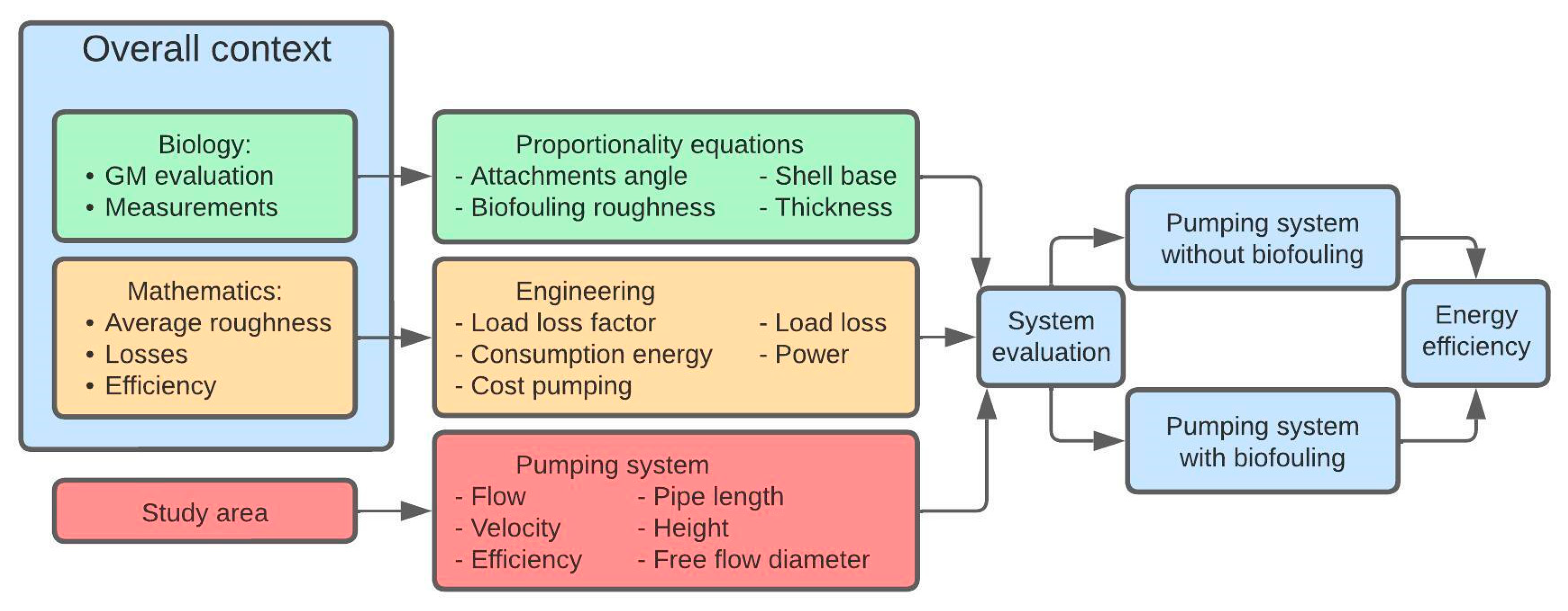
2.1. Overview
This study includes an assessment of the loss of energy efficiency in a pumping system of a known pumping station under the golden mussel (GM) biofouling hypothesis. Some biological information from the GM, constructive data from the target station, and some mathematical engineering parameters were used, all of which influence the performance of the pumping system (e.g., load loss). This set of information was necessary for the construction of new equations, as well as for the improvement of existing equations and to obtain results on the economic indicators that validate the loss of energy efficiency. An overview of the methodology is presented in
Figure 1, and details of the procedures are reported throughout this section.
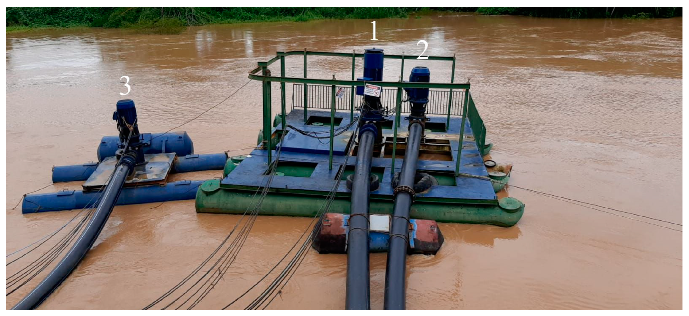
2.2. Local Characterization
To calculate the impacts of biofouling on raw water pumping systems, the Elevated Pumping Station (EPS) II Rio Branco, Acre, Brazil [
36], was used as an example. The extant coordinates of the site are 10° 0′35.95″ S/ 67°50′38.08″ W. A view of the pumping system of the pumping station is shown in
Figure 2. This pumping system is composed of 3 vertical Francis-type centrifugal pumps and a radial rotor that operates 12 h per day, with an average flow rate of 1100 L/s. It has the capacity of vertical mobility by means of floating surfaces, to be able to adjust to the variations in the water levels of the river. The station characteristics considered were flow rate (Q), efficiency (ɳ), power (P), free flow diameter (D), length suction and discharge pipe (L), velocity (V), and height (H) (
Table 1 and
Table 2).
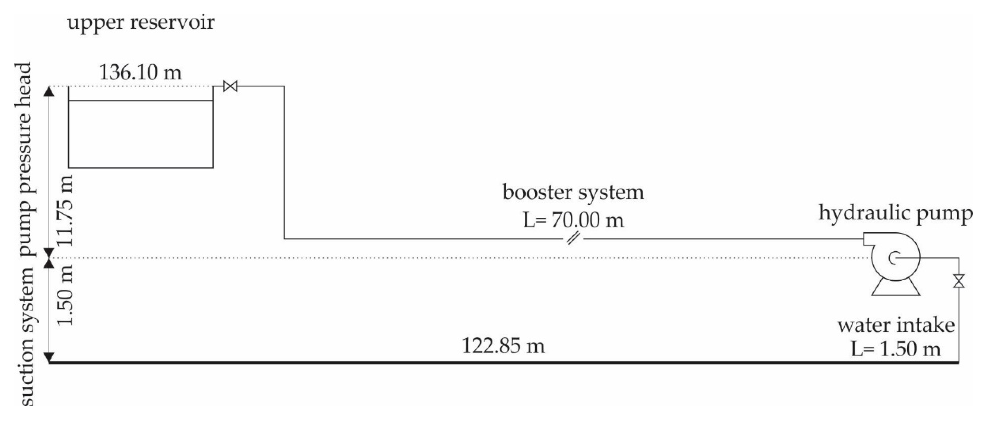
The
EPS that was studied follows the simplified model of a water pumping system (
Figure 3). In this study, calculations were performed considering the weighted average of the river’s elevation quotes. This resulted in a weighted average of 122.85 m and an average gradient of 13.25 m.
2.3. Growth Curve of the Golden Mussel
The growth curve as a function of time and the GM was obtained through data from the literature (
Table 3). It was taken into account that the geometric shape and the location of the attachment in the environment did not have a significant effect on the shell growth of the mussel [
37].
2.4. Determination of the Angle of Attachment and the Proportional Relation between Golden Mussel Individuals
Golden mussels (GMs) were collected in the Itaipu hydroelectric power plant (HPP), which is located in Brazil and Paraguay, 25°24′28″ S, 54°35′24″ W. The GM decomposes rapidly after being removed from the water; accordingly, it was decided to work with dried and sterilized shells. The measured parameters and the angle of attachment were as described by Mackie and Claudi (2010) [
41] and Froés et al. (2012) [
42], with modifications.
The sample of dried shells containing 1000 specimens of GM went through quartering separation, according to the recommendations of the Brazilian Technical Standard ABNT NBR 10007 [
43]. This sample was subdivided into 7 classes, separated according to the shell length of the bivalve, as follows: 0–5 mm, 5–10 mm, 10–15 mm, 15–20 mm, 20–25 mm, 25–30 mm, and >30 mm. Three subsamples, containing 5 individuals in each class, were separated to take the measurements, as shown in
Figure 4. After measuring the individuals, the angle of attachment was determined (
Figure 4). Then, the rest of the dry shells were artificially attached to surfaces with glue (ASTM-A36 steel), with different materials used in different parts of the HPPs, as reported and used by Simeão (2011) [
44]. These artificial attachments were based on the angles of attachment, reproducing the GM attachments that occur in the field. The ASTM-A36 steel surfaces to which shells were artificially attached were photographed for further analysis (see below).
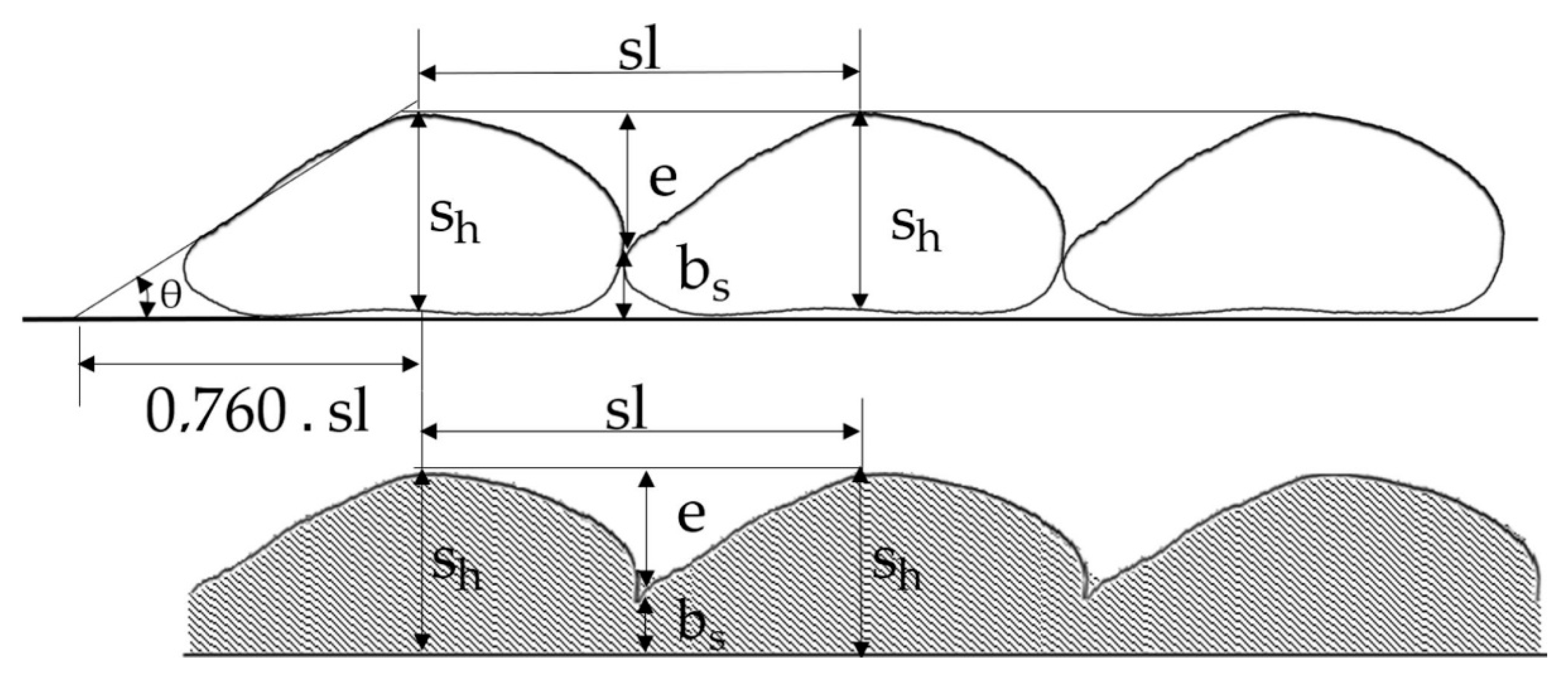
The three previously separated subsamples were examined and their dimensions were surveyed and composed a database containing the dimensions shell length (sl), base shell (bs), shell height (sh) and the angle detachment (θ) for each individual. Thus, it was possible to develop Equations (1)–(4) (new equations). From these data, using the Excel spreadsheet, we obtained a curve that relates the angle “θ” with the “sl” and then adjusted Equation (1), which had a coefficient R² = 0.9935. It was observed by measuring GM husks that the dimension formed between the vertex of the triangle and the top of the bark has a constant ratio of “0.76 · sl” (
Figure 4). Thus, it was obtained from trigonometric relation Equation (2), which provides the dimension “sh”. Dimension “bs,” also obtained by measuring GM shells, corresponds to 38% of shell length “sh” and can be calculated by Equation (3). The “e” corresponds to 62% of the dimension “sh” and can be calculated by Equation (4).
sl: shell length (mm);
: attachment angle (degree);
sh: shell height (mm)
bs: shell base (mm);
e: roughness (mm).
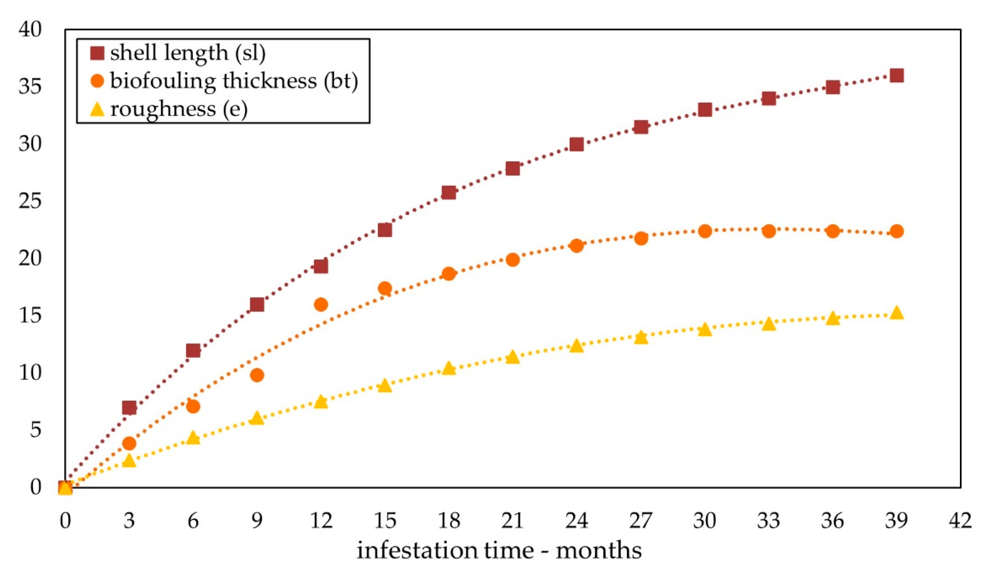
The criteria to determine the thickness of the biofouling were created based on the roughness (Equation (4)) of the surface and calculated without considering the hydrodynamic drag detachment of specimens from the pumping system. This detachment, in turn, was derived from the decrease in the free flow diameter, which was caused by the thickness of the biofouling and the elevation in the velocity flow in the pipe. Thus, using Equation (4), it was possible to determine a characteristic roughness curve as a function of bioinfestation time, allowing for the evaluation of the new flow-free diameters.
2.5. Mathematical Analysis: Calculation of the Thickness of the Biofouling in Pipelines of Average Roughness
With the determination of the shell height using Equation (2), it was possible to calculate the thickness of the biofouling, according to the hydrodynamic drag detachment. However, it is important to consider the interference of flow velocity in the progression of biofouling in pipelines. Based on the studies of Castro (2013) [
45], it is assumed that the velocity effect gradually increased the detachment of the mussels. A detachment of 20% of the thickness of the biofouling is seen between the speed ranges 2.0 m/s and 2.5 m/s. Thereafter, a detachment of 40% is found between 3.0 m/s and 3.5 m/s, advancing to 60% between 3.5 m/s and 4.0 m/s, and to up to 80% at velocities above 4.0 m/s. When the velocity reaches 4.5 m/s, all new specimens become detached.
Based on the information above, the thickness of the biofouling was calculated related to percentage of detachment, after the beginning of the formation of the second layer of the GM (Equation (5)).
bt: thickness of the biofouling;
: percentage of detachment of the GM.
We assume that, once the value of the thickness of the biofouling exceeds the value of the average roughness of the surface, the second layer of biofouling starts to form.
This creates a pattern for the growth of the layers and makes it possible to estimate the thickness of the biofouling for any time period of infestation. It should be considered that the growth of the GM is not uniform and that the colonies have specimens of various sizes. This leads the average roughness to be affected by the diversity of these specimens.
The parameter chosen to obtain the roughness caused by biofouling was the average roughness (
), which is a parameter applied in most engineering processes [
46,
47]. To determine the Ra using Equation (6), photographs of the surfaces (ASTM-A36 steel) with artificially attached dried shells were used (see
Section 2.4). On each surface (nine), a midline was drawn (from the mussel fixation base), through which measurements were made between peaks and valleys, as described in Han et al. (2019) [
48].
: average roughness (mm);
: number of measurements taken;
2.6. Load Loss
Since biofouling occurred on the entire inner surface of the pipe, the free flow diameter (D) in the pipe was decreased by twice the value of the thickness of the biofouling.
The velocity flow inside the pipes was obtained from the data of the EPS studied [
36]. The reduction of the diameter was based on the thickness of the biofouling and was calculated by using the equation of continuity, Equation (7) [
49].
Q: flow rate (m³/s);
A: area of the pipeline ().
In order to calculate the load loss factor (
), a function was defined, using Equation (8), Buzzelli’s Equation [
50]. This equation contains two roots:
obtained using Equation (9), and
Equation (10), obtained as a function of
(average roughness), D (free flow diameter), and the Reynolds number (Re), which was obtained from Equation (11) [
49]. All calculations were carried out considering two scenarios: a pumping system without biofouling and a pumping system with biofouling. The value of the roughness of the pipe surface (ASTM-A36 steel), was considered as
[
17], which was the value considered for the system without biofouling.
f: load loss factor;
B1: root 1;
B2: root 2;
Re: Reynolds number;
D: free flow diameter (m);
: kinematic viscosity of water, .
With the values obtained above, the load loss was calculated using the Darcy–Weisbach equation, Equation (12) [
51].
: load loss (mca);
L: pipe length (m);
g: gravity acceleration —.
To determine the total height of the elevation, or the total load loss of the pumping system, Equation (13) was used [
51].
: total height of the elevation (mca);
: the average geometric gradient to be compensated for (mca);
: sum of the load loss due to suction and the discharge pipe (mca).
The load loss due to suction and the discharge pipe was calculated using Equation (14) [
51].
The methodology used here to calculate the load loss was also described by Mataix (2009) [
49].
2.7. Energy Efficiency
The pumping power needs to be known for the calculation of the economic cost of pumping. Equation (15) [
51], shown below, considers the yield of the pumps as described by Mataix (2009) [
49] and the water working fluid at atmospheric pressure.
P: pumping power (kW);
: water-specific weight ();
: efficiency.
The consumption, of the pumping system without bioinfestation, taking into account the potency obtained for said system was obtained using Equation (16) [
49].
: consumption of the pumping system without bioinfestation (kWh);
: power calculated for the pumping system without bioinfestation (kW);
: number of operating hours of the pumping system in hours, days, or years.
The consumption of the pumping system with bioinfestation, taking into account the potency obtained for said system, was obtained using Equation (17), [
49].
: consumption of the pumping system with bioinfestation (kWh);
: power calculated for the pumping system with bioinfestation.
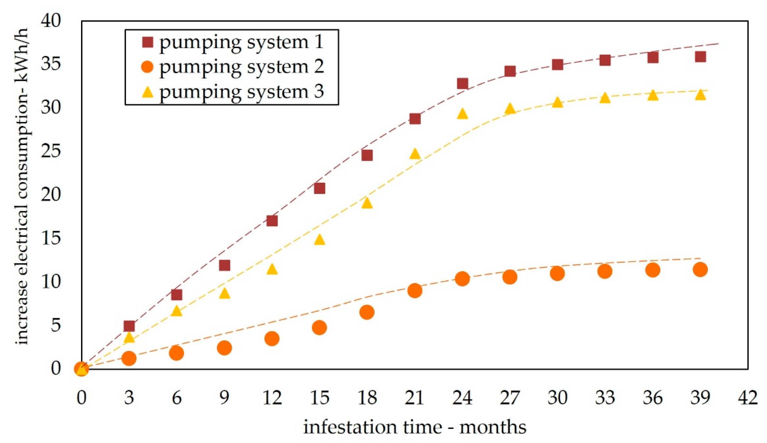
The increase in energy consumption by hour is the value of the difference in power between the systems with and without biofouling, multiplied by the pumping operation time. This calculation is given as Equation (18) (improved equation) [
49].
The costs of the pumping system per cubic meter without bioinfestation were obtained via Equation (19) [
49], in view of the consumption of the pumping system and of the volume that was pumped
: cost of pumping per cubic meter before infestation (USD/m³);
: volume that was pumped (m³);
Price: price per kWh (USD/kWh).
The cost of the pumping system per cubic meter with bioinfestation was obtained by using Equation (20) [
49], in view of the consumption of the pumping system with bioinfestation and of the volume that was pumped.
: cost of pumping per cubic meter after bioinfestation (USD/m³).
4. Conclusions
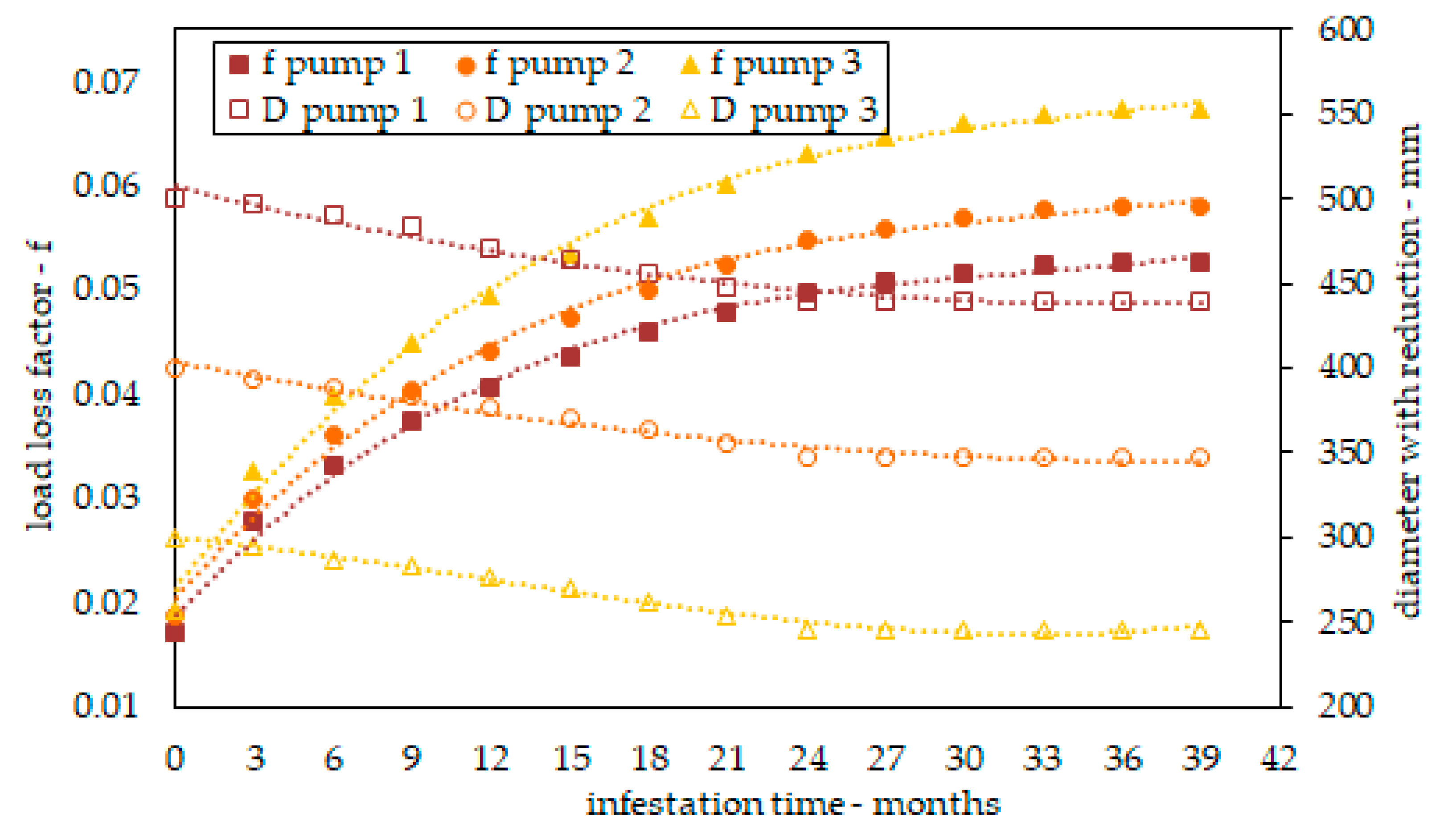
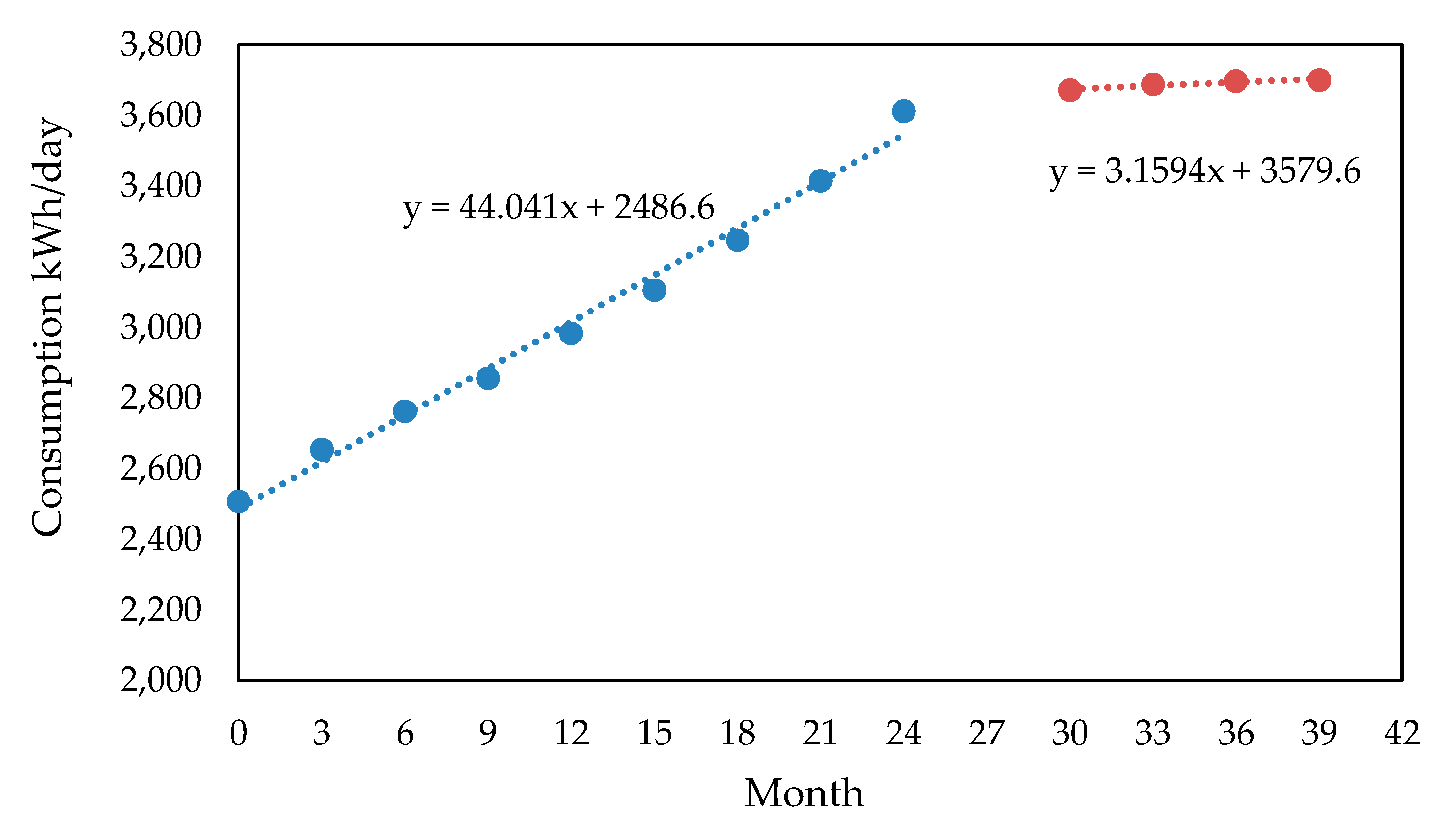
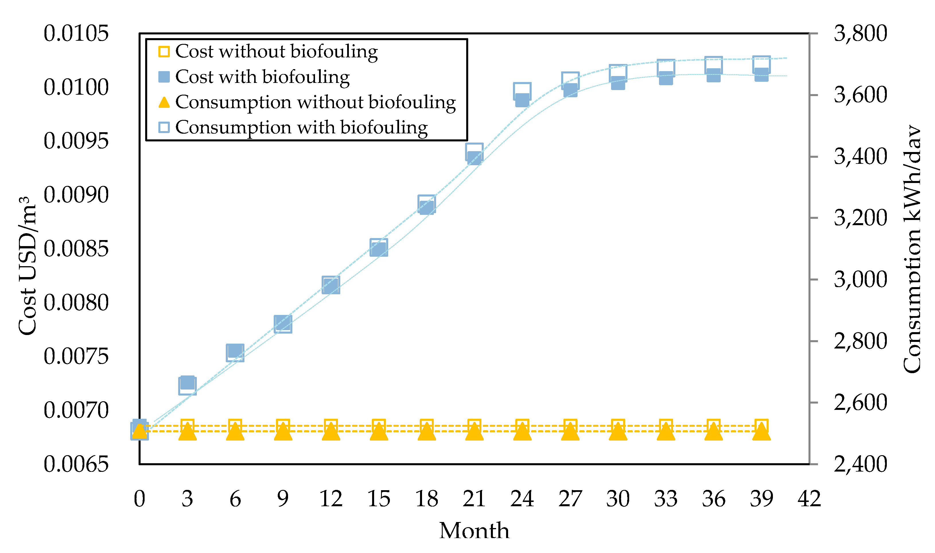
The methodology used was appropriate for the analysis of energy efficiency related to the presence of the golden mussel (GM) in a water pumping system. The complexity of the methodology, including the use of classical equations and the construction of new ones, allowed all of the objectives of this work to be achieved, even without the analysis of all the variables commonly used in the calculation of energy efficiency. Shell growth increases in the first year, and after that period, it suffers reductions in growth rate of 50% per year, stabilizing after the third year of life. This growth rate was corroborated by data from the literature and provided validation for the methodology of proportional relations between the measures performed in the target GMs. This was the starting point for the construction of new equations (three new equations), which allowed for the construction of roughness and thickness curves for biofouling, proving for the first time the relationship between the three elements (shell growth, roughness, and thickness of biofouling). The interference of hydrodynamic drag (flow velocity) was fundamental for the above conclusion, since it causes the detachment of individuals, interfering with the progression of GM fixation (biofouling thickness). In fact, the thickness of the biofouling suffers velocity interference, and this has also been pointed out in the literature. In this study, we show that velocities above 3.8 m/s prevented increased biofouling thickness. This is important for the definition of mussel control and management strategies in pumping systems by controlling flow velocity. Another relevant point was that the size of the individuals did not directly interfere with the increase in roughness, but rather, with the formation of colonies (increased density, number of individuals/cm2). This was especially the case for pipes of smaller diameter, where the increase in density represented a large increase in the load loss factor, proving that bioinfestation (an increase in biofouling thickness) causes a reduction in the efficiency of the pumping system by decreasing the flow diameter. This reduction in diameter causes an increase in energy consumption so that the same flow is achieved. We consider the cost of biofouling for other industrial plant systems, for example, to be much higher than that presented here (almost 46% for 30 months of infestation), since the calculations were made for only one water treatment plant, with simple mechanical fluid systems (when compared with an HPP, for example) and without taking into account localized losses, which would cause an even greater increase in the costs of pumping. As an alternative to the problem presented, performing stops during the operation of the pumping system for corrective maintenance would be the first option, avoiding an increase in operational costs. Another option could be adopting selective pumping criteria, which prioritize pumps and systems with larger diameters, since these are less impacted by GM biofouling. The application of this strategy in our case study could have meant a reduction in the operation time of Pump 3, since this pump is connected to a pipe with a smaller diameter (300 mm) than the other two pumps studied. To compensate, Pumps 1 or 2 could stay activated for a longer time. This way, the pump that was most affected by the bioinfestation, Pump 3, could serve as a backup. Measures such as regular pumping system inspections reduce the advancement of GM bioinfestation, preventing an increase in operational costs. Considering that this study focuses on the water supply and distribution sectors of the Amazon region, we call attention to the negative impacts of GM bioinfestation and provide possible ways to deal with this situation. Linked to these characteristics, bioinvasion would be very harmful for this type of pumping system, due to the morphology of the uptake and the difficulty of maintenance. Here, we provide results that demonstrate the energy efficiency of pumping systems impacted by the golden mussel.

 ,
, 


