Article

Numerical Analysis of Aerodynamic Thermal Properties of Hypersonic Blunt-Nosed Body with Angles of Fire

1
College of Mechatronic Engineering, North University of China, Taiyuan 030051, China
2
Key Laboratory of Aerospace Thermophysics of Ministry of Industry and Information Technology, School of Energy Science and Engineering, Harbin Institute of Technology, Harbin 150001, China
*
Author to whom correspondence should be addressed.
Energies 2023, 16(4), 1740; https://doi.org/10.3390/en16041740
Submission received: 26 December 2022 / Revised: 25 January 2023 / Accepted: 7 February 2023 / Published: 9 February 2023
(This article belongs to the Special Issue Numerical Simulation on Heat Transfer Technique)

Abstract

:
A hypersonic electromagnetic railgun projectile undergoes severe aero-heating with an increase in altitude. The purpose of this study was to investigate the characteristics of the shock layer flow field as well as the thermal environment of the blunt body wall of a hypersonic electromagnetic railgun projectile at different launching angles. The two-temperature model considers the thermal nonequilibrium effect and is introduced into the Navier–Stokes (N-S) equation, and it is solved using the finite volume method (FVM). The reliability of the calculation model in terms of thermal properties and composition production was verified against a blunted-cone-cylinder–flare (HB-2) test case. The surface temperature of the hypersonic blunt projectile was simulated using a radiation balance wall boundary. The thermal characteristics at the emission angles α = 60° and α = 45° were checked within an altitude range of 0–70 km, including the nonequilibrium effect, reaction heat release, aerodynamic heat flux, and wall temperature. The results show that the translational rotational temperature is higher than the vibrational electronic temperature, and the thermal nonequilibrium effect increases with an increase in altitude. Comparing the two launching angles, the nonequilibrium degree and reaction heat release at α = 60° were higher than those at α = 45°. The rates of exothermic reaction decreased with an increase in altitude. The heat flux along the wall of the generatrix decreased sharply from the stagnation point. With an increase in altitude, the heat flux dropped sharply from 7 MW/m2 at H = 0 km to approximately 2 MW/m2 at H = 70 km. The wall temperature distribution was similar to the heat flux distribution; however, the surface temperature decreased less rapidly than the heat flux.

1. Introduction

An electromagnetic launch (EML) is a technology that uses electromagnetic energy to accelerate and launch projectiles [1,2]. Devices that use EML technology to launch projectiles are generally referred to as electromagnetic guns. The most important application of electromagnetic guns in the military are line-of-sight armor-piercing weapons and long-range suppression weapons [3]. At present, the direct kinetic energy penetration of high-speed projectiles is the main method to strike solid defense targets. An electromagnetic gun fires a projectile at a much higher initial velocity than that of a conventional gun. Not only does it improve the armor-piercing ability, but also considerably reduces the mass and volume of ammunition and improves the carrying capacity of weapon systems [4]. In addition, electromagnetic guns can achieve several times the speed and range of conventional guns.
The projectile of an electromagnetic gun is launched at hypersonic initial conditions (>Mach 5). The US Naval Surface Warfare Research Center conducted a series of experiments with an electromagnetic railgun [5]. The aluminum bullet, weighing 3.35–3.36 kg, was launched with 10.68 MJ export kinetic energy, the export speed was 2.5 km/s, and the kinetic energy was 10 MJ. Subsequently, the US Navy announced that it had successfully conducted a new round of electromagnetic gun tests, with a projectile mass of 10.4 kg, muzzle velocity of 2.5 km/s, and kinetic energy of 33 MJ [2]. In the 2015 US Navy plan, it was pointed out that the electromagnetic railgun performance accelerates the 20 kg projectile to 2.5 km/s.
When the electromagnetic projectile flies at a hypersonic speed, the temperature of the surrounding gas rises sharply, forming a high-temperature flow field due to the viscous stagnation of the gas and the compression of the shock wave. The vibration excitation of gas molecules occurs in the high-temperature environment of aerodynamic heating, accompanied by a series of complex physical and chemical processes such as dissociation, chemical reaction, ionization, etc. [6]. The flow around shows the characteristics of the thermochemical nonequilibrium effect [2,3], which makes the aerodynamic thermal environment of hypersonic vehicles more complex. The velocity of hypersonic projectiles is large, often reaching 2000 m/s and above. At such a high flight velocity, there is a very serious aerodynamic heating phenomenon on the surface of the projectile. Aerodynamic heating causes the surface temperature of the projectile body to rise, and even ablation occurs on the surface of the projectile body after reaching a certain temperature [7]. The thermal ablation effect may cause a change in the projectile configuration of the electromagnetic track gun. Furthermore, the change in hypersonic projectile geometry may not only increase the resistance, but also cause non-design forces and moments affecting the stability, which has a certain impact on the precise strike of the projectile [8]. Therefore, the aerodynamic thermal prediction and thermal protection technology of hypersonic projectile surfaces has become one of the key technologies in the development of this kind of projectile.
After the projectile leaves the acceleration electromagnetic railgun at a hypersonic speed, the flight trajectory is determined by the initial velocity, initial inclination, gravity, and aerodynamic drag [9]. For an electromagnetic railgun with a fixed launching capacity, the initial kinetic energy of the projectile is constant, which means that the initial velocity is a fixed value. For a projectile with a fixed configuration, a difference in the initial launching angle causes an obvious difference in trajectory. The existing numerical studies on the aerodynamic and thermal properties of electromagnetic rail gun modeling are mostly based on the single-temperature model in thermodynamic equilibrium state. Most work focus on the influence of aerodynamic configuration by numerical analyses considering one or several typical calculation points. For example, Shen et al. [10] applied the steady computational fluid dynamics (CFD) simulation method to obtain the characteristics of the electromagnetic gun projectile flow field at different Mach numbers, and used them to optimize the aerodynamic shape of the projectile in hypersonic conditions. Kasahara et al. [11] studied the geometric effect of electromagnetic rail projectile under stable flight conditions in thermal equilibrium states. Rahman et al. [12] used the single-temperature CFD method of steady compressible flow to simulate the density, pressure, and temperature flow fields of an electromagnetic projectile at different Mach numbers (5~10).
At present, the aerodynamic and thermal properties along the flight trajectory are seldom studied. The thermal nonequilibrium effect of the gas in the shock layer should not be ignored for a hypersonic vehicle with an increase in flight altitudes. As the altitude increases, the density of the atmospheric environment drops and the free path of molecules increases sharply [13]. This means that the thermodynamic equilibrium state of air species requires a certain relaxation time to reach. At present, the aerodynamic numerical calculation of electromagnetic railgun projectile mostly assumes that the high-temperature gas is in a thermodynamic nonequilibrium state. Under the action of high-speed inflow, chemical reactions such as the dissociation and recombination of gas also experience a chemical nonequilibrium state at a high temperature. Sarma [14] pointed out that a high-speed flow experiences different flight corridors under different combination conditions of speed and altitude to prevent severe aerodynamic thermal effects. Niu et al. [15] also found that hypersonic flows under different flight conditions show typical thermodynamic nonequilibrium characteristics and affect the thermal behavior of the shock layer. Therefore, the aerodynamic and thermal characteristics of projectiles with different launch angles are calculated based on the thermochemical nonequilibrium two-temperature model.
Due to the high cost of flight test and ground wind tunnel test, effective test data are relatively scarce. Therefore, numerical simulation is an indispensable tool in the basic research of hypersonic flow. It is necessary to simulate the thermal state of electromagnetic railgun projectiles at different angles of fire by numerical methods. From the point of view of the selection of electromagnetic railgun parameters, the objective of this study is to examine the thermal properties of the corresponding exterior ballistics of the projectile at different angles of fire, including nonequilibrium effect, reaction heat release, aerodynamic heat flux, and wall temperature. The remainder of this paper is organized as follows: Section 2 provides the descriptions of the thermal effect of the blunt body. Section 3 introduces the numerical models for the thermal properties of hypersonic flow. Section 4 presents the validation of the numerical models. Section 5 provides the computation details, and Section 6 analyzes and discusses the thermal properties of the electromagnetic railgun projectile. Finally, the last section presents the concluding remarks.

2. Thermal Effect of Blunt Body

For hypersonic projectiles, the body is typically designed as a slender blunt cone. For flight stability, tail wings are symmetrically distributed along the axis and installed at the tail of the projectile body. The projectile configuration is shown in Figure 1. The projectile was launched on an electromagnetic railgun, and its wingspan was the same as that of the launch caliber. The projectile drags were wrapped outside as they were required to accelerate the launch of the rail. To achieve the universality of weapons and equipment, projectiles can be accelerated in the same fixed-caliber barrel to adapt to different launch platforms. To design the projectile configuration, it is necessary to consider the aerodynamic heating effect of the projectile corresponding to the blunt cone configuration of the projectile body. In addition, the projectile launched by the electromagnetic railgun can have not only a straight or parabolic trajectory, but also an approximate vertical trajectory. This implies that hypersonic projectiles may experience different flow states during flight. The environmental atmospheric characteristics were significantly different under different flow conditions. An interesting problem in engineering applications is the question of the thermal characteristics of the projectile and the flow field around the projectile change when different blunt cones fly at a particular altitude.

3. Physical Model and Numerical Method

3.1. Governing Equation

In the three-dimensional Cartesian coordinate system, the conservative integral form of the compressible Navier–Stokes equation can be written as [16,17]:
t Ω Q d Ω + Ω F j F v , j d S = Ω ω ˙ d Ω
where Ω is the control volume and ∂Ω is its elemental area. Q is the conservative variable, and Fj and Fv,j are the components of convective and viscous fluxes in the jth direction, respectively. ω ˙ is the source term.
For the thermochemical nonequilibrium gas, vectors above can be expressed based on Park’s two-temperature model [17] as follows:
Q = ρ 1 ρ N s ρ u i E E v e ,   F j = ρ 1 u j ρ N s u j ρ u u j + p δ i j E + p u j E v e u j , F v , j = ρ h 1 D 1 y 1 x j ρ h N s D N s y N s x j τ i j τ i j u i q t r , j + q v e , j h s D s y s x j q v e , j e v e , s D s y s x j , ω ˙ = ω ˙ 1 ω ˙ N s 0 0 ω ˙ v e
where Ns is the maximum number of species s. ui is the macroscopic flow velocity components in the ith direction. ys and Ds are the mole fraction and diffusion coefficients of the species s. hs is the enthalpy of the chemical species s. δij is the Kronecker delta. E and Eve represent the total energy per unit volume and the vibrational–electronical energy per unit volume of the mixture, respectively.
The mixture pressure p can be calculated by Dalton’s law of partial pressures [18]:
p = s = 1 N s ρ s R M s T t r + ρ e R M e T v e
where R represents the universal gas constant. In the two-temperature model, the temperature can be characterized by the translational–rotational temperature Ttr and the vibrational–electronical temperature Tve. M is the molecular weight of species.
The thermal flux from the translational–rotational energy and the vibrational–electronical energy in the j direction are described by qtr,j and qve,j:
q t r , j = η t r T t r x j   and   q v e , j = η v e T v e x j
where η is the thermal conductivity coefficient of the mixture.
The viscous stress tensor of a Newtonian fluid, τij, is defined as:
τ i j = μ u i x j + u j x i 2 3 μ β u k x k δ i j
where μ is the molecular viscosity coefficient and β is the bulk viscosity coefficient.

3.2. Source Term

In the governing equation, the vector of the source term as given in Equation (2) includes two terms: one is the chemical reaction source term in the continuity equation, and the other is the energy mode source term in the energy conservation equation for the vibrational–electronic mode. The mass production rate per unit volume for species s has the following form:
ω ˙ s = M s r = 1 N r β s , r α s , r R f , r R b , r
where αs,r and βs,r are the stoichiometric coefficients of species s in the rth reaction for reactants and products, respectively. Nr is the number of reactions related to species s. Rf,r and Rb,r are the forward and backward reaction rates, which can be written as follows:
R f , r = k f , r s = 1 N s ρ s M s α s , r
R b , r = k b , r s = 1 N s ρ s M s β s , r
where kf,r is the rate constants of the forward reaction and kb,r is the rate constants of the backward reaction for the rth reaction.
In the two-temperature model, there is a relaxation process for all kinds of energy to adjust from nonequilibrium state to equilibrium state due to thermodynamic nonequilibrium effects. In the absence of radiation, the exchange of energy is mainly achieved through molecular collisions. Therefore, the internal or vibrational energy source term with the vibrational relaxation time has the following form [17]:
ω ˙ v e = s = 1 ρ i e v e ( T ) e v e , s ( T v e ) τ v e + s ω ˙ s e v e , s
where the average relaxation time τ v e can be calculated by the Milikan–White’s semi-empirical formula [19]. The internal energy per unit of mass e v e , s can be given by:
e v e , s = r = 1 N d g s , r θ v e , s , r exp θ v e , s , r / T v e 1 R M s
where θve is the characteristic vibrational temperature and Nd is the number of degeneracy states.

3.3. Transport Properties

In the two-temperature model, the transmission characteristics of components in each energy mode can be calculated by the Gupta mixing rule [20], including dissipation, viscosity, and heat conduction. The effective mixture diffusion coefficient can be given by:
D s = γ t 2 M s 1 ρ s ρ s = 1 s s N s γ s / D s s
where γs is the molar concentration of species s. Dss’ represents the binary diffusion coefficient between heavy particles s and s’, which can be expressed as:
D s s = k T p Δ s s ( 1 ) ( T )   and   γ t = s = 1 N s γ s
where k is the Boltzmann’s constant. Δ s s ( 1 ) ( T ) is the collision integrals related with collision pairs of particles.
According to the basic theory of molecular motion theory and statistical thermodynamics, the calculation formula of the macroscopic thermal conductivity of each energy mode in the mixed gas can be derived. The translational, rotational, vibrational, and electronic thermal conductivities are defined as ηt, ηr, ηv, and ηe. The thermal conductivities of the mixed gas in two models are given by [16]:
η t r = η t + η r
η v e = η v + η e
where
η t = 15 4 k s = 1 s e N s γ s s = 1 s e N s a s s γ s Δ s s ( 2 ) T t r + 3.54 γ e Δ e s ( 2 ) T v e
η v = η r = k s = m o l . N s γ s r = 1 r e l e c t r o n N s γ r Δ s s ( 1 ) T t r + γ e Δ e s ( 1 ) T v e
η e = 15 4 k γ e s = 1 N s 1.45 γ s Δ e s ( 2 ) ( T v e )
where Δ s s ( 2 ) ( T ) is the modified collision integrals, for which parameters can be seen in Ref. [20].
The mixture viscosity can be expressed as:
μ = s = 1 s e N S m s γ s s = 1 s e N s γ s Δ s s ( 2 ) T t r + γ e Δ e s ( 2 ) T v e + m e γ e r = 1 N s γ s Δ e s ( 2 ) T v e

3.4. Thermodynamic Properties

For high-speed and high-temperature flows, the translational energy, rotational energy, vibrational energy, and electron energy of the molecule are all or partially excited. The internal energy of the excited gas molecules has an effect lagging the equilibrium state for the thermal nonequilibrium gas. In the two-temperature model, it is assumed that the translational energy and the rotational energy of the gas molecules are fully excited at the temperature range of 200–20,000 K. The thermal properties can be expressed in polynomial forms:
C p , s R = k = 1 5 A k s T k 1
h s R T = k = 1 5 A k s T k 1 k + A 6 s T
G s R = A 1 1 ln T k = 2 5 A k s T k 1 k 1 k + A 6 T A 7
where Cp,s is the specific heat of species s at constant pressure, hs is the specific enthalpy of species s, Gs is the free energy of species s at standard pressure, and A1A7 are constants which have been tabulated in Ref. [20] for various temperature ranges.
The contribution of these temperatures is different depending on the number of atoms in a molecule. For 7 species air, e-, N, NO, NO+, N2, O, and O2, the thermodynamic properties can be divided into two types. Due to no rotational degree of freedom for atoms, the contribution of translational–rotational temperatures is 5R/2 for atoms and 7R/2 for diatomic molecules [20].
For atoms:
C p , s , t = 5 2 R ,   C p , s , r o t = 0 , h s , t = 5 2 T R + A 6 R ,   h s , r o t = 0
For diatomic molecules:
C p , s , t = 5 2 R ,   C p , s , r o t = R , h s , t = 5 2 T R + A 6 R ,   h s , r o t = T R
The vibrational–electronical part of the specific heat at constant pressure and enthalpy can be written by [18]:
C p , s T v e = C p , s T v e C p , s T t C p , s T r o t
h s T t r , T v e = h s T v e + C p , s , t + C p , s , r o t T v e + T r e f + h s , 0
where T is the integral variable and Tref is the reference temperature of 298 K. hs,0 is the enthalpy of species s, which are provided in Refs. [21,22].

3.5. Chemical Reaction Model

In most cases, the equilibrium rate constants are obtained in the thermodynamic equilibrium, which is expressed as a function of temperature T. However, under the condition of low density and high energy, the assumption of thermodynamic equilibrium is not valid. Comparing the characteristic time chemical reaction with the vibration relaxation time, it is advised to introduce the coupling effect between these characteristic times into the controlling temperature. In thermal nonequilibrium conditions, the assumption of a single rate-controlling temperature is made for certain classed of reactions. For dissociative reactions, the rate controlling temperature, Tc is written as:
T c = T a T v e b
where a and b are the power law coefficients.
For ionization reactions of electron impact, the controlling temperature is the vibrational–electronical temperature Tve. The rate constants of the forward and backward reaction, kf,r and kb,r in Equation (7), are determined by the Arrhenius relationship [23]:
k f , r = A f , r T c n f , r exp E f , r / k T c
k b , r = A b , r T c n f , r exp E b , r / k T c
where A represents the frequency factor, which is obtained from normalization on the thermal reaction rate. Tc is the controlling temperature, n is the temperature exponent, E is the activation energy, and k is the Boltzmann constant (1.38054 × 10⁻²³ J/K).
In the present study, a 7-species chemical kinetics reaction borrowed from the Park 93 [24] model is used. Forward chemical kinetic rate coefficients are shown in Table 1, where M1, M2, and M3 represent the third body. In dissociation reactions, the third body can be any species in the reaction system, which are provided in Ref. [24].
In the present study, the forward rates in electron impact dissociation are determined by the vibrational–electronic temperature. For the backward rate in the electron impact dissociation reactions, the use of a geometric average expression is widely accepted. The reaction type and the weight factors of the forward and backward rates are listed in Table 2.

3.6. Turbulence Model

In the present work, Favre averaging was used with the governing equation to evaluate turbulent fluctuations. A two-equations standard k-ε turbulence model was used to calculate the hypersonic flow field in this paper. This turbulent model has good robustness and reasonable accuracy, and has been widely used. It is based on turbulent flow energy k and dissipation rate ε. The compressible modified turbulence model is used in the real gas model to consider the turbulence effect. Turbulence kinetic energy and inverse time-scale transport equation are written as [25]:
ρ k t + x j ( ρ k u j ) = x j μ + μ t σ k k x j + G k G b ρ ε ϕ
ρ ε t + x j ( ρ ε u j ) = x j μ + μ t σ e ε x j + C 1 e ε k G k + C 3 e G b C 2 e ρ ε 2 k
where Gk is the turbulent kinetic energy generated by the average velocity gradient. Gb is the turbulent kinetic energy generated by buoyancy. ϕ is the contribution of wave expansion to total dissipation rate in compressible turbulence. C, C, and C are constants, whose values are 1.44, 1.92, and 0.09, respectively. σk and σε are the turbulent Prandtl number for turbulent flow energy k and dissipation rate ε, which are assigned as 1 and 1.3, respectively.

3.7. Computational Method

The governing equations were discretized with the finite volume method (FVM) [26] based on multi-block structured grids. To capture the supersonic shock layer accurately, Yee’s Symmetric Total Variation Diminishing (STVD) scheme [27] was used for the treatment of the convective flux, which has a good performance in stability and the accuracy for the solution of hypersonic flows. Note that a non-physics result may exist when the Jacobian matrix has a very small eigenvalue. Harten’s entropy correction functions [28] are thus applied to add some dissipation. The vector of the viscous flux is calculated by the center difference scheme [29].

4. Validation of Numerical Models

To verify the hypersonic calculation model in predicting thermal characteristics, a test case blinded cone cylinder plane designed HB-2 [30] was used as a validation study. The force and heat transfer of the HB-2 test model under different free flow conditions were carried out in various test facilities, such as the Japan Aerospace Exploration Agency (JAXA) and Arnold Engineering Development Center (AEDC). The geometric dimensions of the HB-2 test model are shown in Figure 2a.
To accurately capture the heat transfer and pressure on the surface, a sufficiently fine computational grid is required. The accuracy of heat transfer prediction near the wall depends largely on the quality of the grid and the clustering near the wall. The number of transverse and longitudinal grids is 100 × 200, respectively, and the Reynolds number of the first grid near the wall is less than 2. In Figure 2b, the grid distribution of the computational domain required for numerical calculation is shown. The free stream boundary conditions used for this test case are supersonic inflow and exit. On the wall, the slip-free isothermal surface T = 300 K is specified, and the normal and transverse velocity components of the wall are zero. The symmetry condition is applied along the cone axis. These conditions are derived from the experimental data obtained from the VKF and JAXA test facilities.
Figure 3 shows the comparison between the calculated values and the experimental measurements of the characteristic parameters along the surface. Figure 3a,b show the pressure and heat flux distributions respectively, and their corresponding parameters are dimensionless using the stagnation point values. The results show that the calculated values of the current numerical model are in good agreement with the experimental data. Additionally, nitrogen and oxygen molecules dissociate to form nitrogen and oxygen atoms, respectively. Oxygen molecules are almost completely dissociated to form oxygen atoms in a high temperature. In addition, oxygen and nitrogen atoms combine to form NO molecules. Figure 4a,b show the comparison of the temperatures along the hysteresis line and the main air-dissociated components between the numerical calculation results and reference data [31], respectively. The results verify the reliability of the current calculation model in the prediction of species and thermal properties.

5. Design of Numerical Experiment and Computation Details

5.1. Geometry of Blunt Body

Referring to the configuration of the hypersonic projectile adopted by the US Navy’s electromagnetic railgun, a projectile approximate to its configuration was used as the research object of this paper. The projectile was about 660 mm long and the wingspan of the tail was 155 mm. The projectile was suitable for various launching platforms of 155 mm caliber barrel, and the diameter of the rear end of the projectile was 120 mm. Except for the tail fin, the projectile was designed as a blunt cone. We considered that the most serious thermal effect is in the front section of the blunt body during flight. Therefore, this paper only focuses on the flow field and wall thermal effect in a certain distance from the front of the blunt body, as shown in Figure 5. According to the configuration of the electromagnetic projectile, the nose radius of the blunt cone concerned in the numerical calculation was 5 mm, the half cone angle was 4.8°, and the length of the precursor was 0.1 m.

5.2. Mesh and Boundary Conditions

At zero angle of attack, the axisymmetric domain can be used to calculate the flow field of the blunt cone. The computing domain grid was divided by the commercial software ANSYS-ICEM, and the grid distribution is shown in Figure 5. The number of radial and axial grids in the grid is 85 × 175, and they were structural quadrilateral grids. The Reynolds number of grids is widely used to ensure the accuracy of wall heat flow prediction in high-speed flow. Previous studies have shown that the grid spacing perpendicular to the wall direction should ensure that the grid Reynolds number is less than 2. In this paper, the size of the first layer of the grid near the wall, namely the size of the smallest cell, was 1 × 10⁻⁶ mm.
Four boundary conditions are required for flow field calculation, including inlet, the axis of symmetry, outlet, and wall boundary conditions. Among them, the inflow boundary specifies uniform inflow velocity, pressure, and temperature parameters, and the inflow parameters corresponding to different ballistic calculation points are shown in Section 5.3. Given the projectile is hypersonic, the exit boundary of the computational domain can be derived from the upstream supersonic flow field parameters. The wall was designated as a radiation equilibrium boundary condition without slip, catalysis, and ablation effects.

5.3. Computational Cases

Assuming that the projectile launched by the electromagnetic railgun meets the 43 resistance law, the ideal trajectory of projectile flight can be obtained under the following simplified conditions: (1) the shape and mass distribution of the projectile are axisymmetric bodies, and the angle of attack is zero, (2) the flight environment is a standard meteorological condition, (3) the influence of Coriolis inertial force and the change in gravity acceleration with latitude are ignored, and (4) the change in gravity acceleration with altitude is ignored. Based on the above assumptions, the exterior ballistic equations can be established.
Taking the electromagnetic railgun with a 64 MJ muzzle kinetic energy as an example, it was assumed that the conical high-speed rotating projectile was used with a weight of 9 kg, an initial velocity of 3000 m/s, and a shape coefficient of 0.6. In this paper, two firing angles of 45° and 60° were considered. Based on these conditions, the fourth-order Runge–Kutta method was used to solve the trajectory equations. The parameters required for calculating the external ballistic equations are shown in Table 3.

6. Results and Discussions

6.1. Thermal Nonequilibrium Effect of Shock Layer

The altitude concerned in this paper was below 70 km, and the fluid Knudsen number (Kn = λ/L is the ratio of the average free path of the gas molecule to the flow characteristic length) was less than 0.001. This means that the fluid satisfied the continuity assumption. The high-speed incoming flow transformed part of the kinetic energy around the projectile into the internal energy of the air, which made the temperature in the flow field increase to several thousand Kelvins. For high-speed reactive flows, a local thermal nonequilibrium state occurs when the relaxation time of molecular vibration energy is comparable to the flow time in magnitude. In this case, the physical model needed to describe the thermal nonequilibrium effect was different from the single-temperature model. Differently, the multi-temperature model was needed to describe the internal energy conversion and relaxation process between molecules. In this paper, the two-temperature model was used to calculate the flow field parameters, and the flow field temperature was characterized by the translational–rotational temperature and the vibrational–electronic temperature. The difference between the two temperatures can reflect the degree of the thermodynamic nonequilibrium of the flow field, which has the following expression forms:
ϕ = T t r T T v e T
Figure 6 shows the contours of the translational–rotational temperature and the vibration–electron temperature at altitudes of 10 km, 30 km, and 60 km with a α = 60° angle of fire. It can be seen from this figure that the level and distribution of the two temperatures varied significantly with altitudes. Figure 7 shows the two temperature curves along the stagnation line corresponding to representative altitudes. The translational–rotational temperature was higher than the vibrational–electoral temperature, and the thickness of the detached shock wave was also different for two temperature modes. Figure 8 shows the variation curve of the nonequilibrium degree of the flow field parameters along the stagnation line as a function of the altitude of the large value. The degree of thermal imbalance increased with the increase in altitude. This is because the collision probability between molecules decreases with an increase in altitudes, and the molecular vibration needs to be completed through the collision with time history. In addition, the degree of nonequilibrium at α = 60° is higher than that at α = 45°. This is because the freestream velocity at α = 60° is higher than that at α = 45° at the same altitude. In this case, the temperature around the bow shock increased dramatically with the increase in flight speed, and the intermolecular vibration and electronic energy excitation became more significant.

6.2. Reaction Heat Release of Shock Layer

For a hypersonic projectile, the surrounding air is strongly compressed to form a strong bow shock wave. The viscous effect converts the huge kinetic energy in the flow into gas internal energy, which makes the air temperature rise sharply. At high temperatures, the air of the shock layer undergoes a series of complex physical and chemical processes such as dissociation and ionization, accompanied by heat release, component generation, molecular vibrational–rotational transition, electronic excitation transition, etc. The initial temperature of molecular vibration energy excitation is about 800 K. O2 molecules begin to decompose at 2000 K, and O2 is completely decomposed at 4000 K. At this temperature range, N2 molecules begin to decompose. When the temperature rises continuously, most N2 molecules decompose into N atoms, and a small amount of NO molecules form with O atoms. This series of physical and chemical reactions and the degree of gas reaction in the shock layer can be characterized by the content of NO formation to a certain extent. In addition, the chemical reaction process releases or absorbs energy with the breaking and recombination of chemical bonds. For the thermal characteristics in the shock layer, the heat released from the chemical reaction of the reaction system can be used to characterize it.
According to Arrhenius’s expression, the generation of NO depends on the control temperature and collision frequency. The literature [32,33] points out that NO is mainly produced by neutral exchange reactions N2 + O ↔ NO + N and NO + O ↔ O2 + N. In these reactions, O2 (or N2) dissociates to produce high-density O (or N) atoms, and then NO is produced between O and N atoms and N2 or O2 due to the above reactions. Influenced by the temperature of the flow field, the mole fraction of NO is mainly distributed in the shock layer region. Figure 9 shows the distribution of NO along the stagnation line corresponding to the six ballistic points. The mole fraction of NO reached the order of 10−10 at H = 10 km. It can be seen from the figure that the concentration of NO along the stagnation line at 10 km in the case of α = 60° was three orders of magnitude higher than that in the case of α = 45°. The content of NO was extremely low at other altitudes, which is related to a low inflow velocity and flow field temperature.
In order to examine the change in heat of different chemical reaction models during the formation of components, the distribution curve of chemical reaction heat in unit volume along the stagnation line is shown in Figure 10. It can be observed that the reaction heat release corresponding to the two angles of fire was significantly different. The reaction heat release at α = 60° was higher than that at α = 45°. The heat release of the reaction decreased with the increase in altitude. This is because the reaction heat release is related to the vibrational–electoral temperature distribution trend, which affects the chemical reaction rate coefficient and the control temperature. These two parameters thus affect the generation of chemical reaction heat release.

6.3. Aero-Heating Effect of Blunt Body

The heating heat flux of the high-temperature flow field towards the projectile surface includes convection heat flux, component diffusion heat flux, and gas radiation heat flux. In this paper, the radiant heat flux of gas is ignored, and the convective heat flux and component diffusion heat flux are included in the flow field calculation. Aerodynamic heat includes heat flux in translational–rotational and vibrational–electronic modes. Figure 11 shows the wall heat flux distribution curve along the external contour of the blunt body at typical ballistic points. It can be seen from the figure that the wall heat flux distribution was the highest at the stagnation point at two selected angles of fire. From the stagnation point, the heat flux along the generatrix of the blunt body decreased sharply. Starting from a position 1.5 times the nose radius downstream of the stagnation point, the heat flux decreased slowly. The heat flux at α = 60°and H = 10 km was up to 8 MW/m2. However, the heat flux was about 3 MW/m2 at α = 45°and H = 10 km. Accordingly, the heat fluxes at α = 60° were higher than those at α = 45° at other altitudes. This is because the free stream velocity is higher at α = 60° than that at α = 45°.
Figure 12 shows the curves of maximum heat flux versus altitude at two launch angles of α = 45° and α = 60°. It can be seen that the maximum heat flux decreased sharply in magnitude under the two angles of fire. The heat flux decreased sharply from 7 MW/m2 at H = 0 km to about 2 MW/m2 at H = 70 km. In addition, the maximum heat flux at α = 60° was higher than that at α = 45°, and the former was about 2 times higher than the latter in the range higher than 20 km. This is because there were significant differences in the inflow conditions corresponding to the two different trajectory calculation points, which inevitably lead to different thermodynamic parameters of the flow field.

6.4. Surface Temperature of Blunt Body

The aerodynamic heat caused by high-speed incoming flow heats the wall, and the heat flux at the wall reaches a balance. In this paper, the radiative wall boundary condition is adopted. The aerodynamic heat flux on the wall mainly consists of convection, dissipative heat flux, and radiant heat flux from the wall to the fluid. Figure 13 shows the wall temperature distribution corresponding to six representative ballistic points at two angles of fire. In this figure, x/Rn = 0 indicates the stagnation point of the blunt body. It can be seen that the wall temperature gradually decreased along the surface of the blunt body in the axial direction, and the temperature was the highest at the stagnation point. The distribution of wall temperature was similar to that of the heat flux. However, the decreasing rate of the surface temperature was not as rapid as that of the heat flux but was relatively slow. By comparing the wall temperature at α = 45° and α = 60°, it can be seen that the temperature difference between two angles at a fixed altitude was basically the same. With the increase in the altitude, the wall temperature difference caused by the angle of fire decreased gradually. For example, the temperature difference is 400 K, 200 K, and 110 K at H = 10 km, 30 km, and 60 km, respectively.
Figure 14 shows the variation curve of the stagnation point temperature with altitudes at two angles of fire. It can be seen from this figure that the maximum temperature decreased significantly with the increase in altitude. Wall temperature at α = 60° was about 20% higher than that at α = 45°. The temperature difference decreased with the increase in altitude. This is due to the comprehensive result that the aerodynamic heat flux on the wall was in balance with the radiant heat flux towards the fluid under two angles of fire, and the freestream velocity was also different at the same altitude.

7. Conclusions

In the current study, the thermal characteristics of hypersonic electromagnetic railgun projectiles at launch angles of 60° and 45° were calculated based on a thermochemical nonequilibrium reaction flow field calculation model. The altitude range of the calculated trajectory point was 0–70 km. The nonequilibrium chemical flow parameters and wall thermal characteristics at different ballistic points were analyzed, including the thermal nonequilibrium effect, reaction heat release, aerodynamic heat flux, and wall temperature. The numerical results revealed the following:
(1)
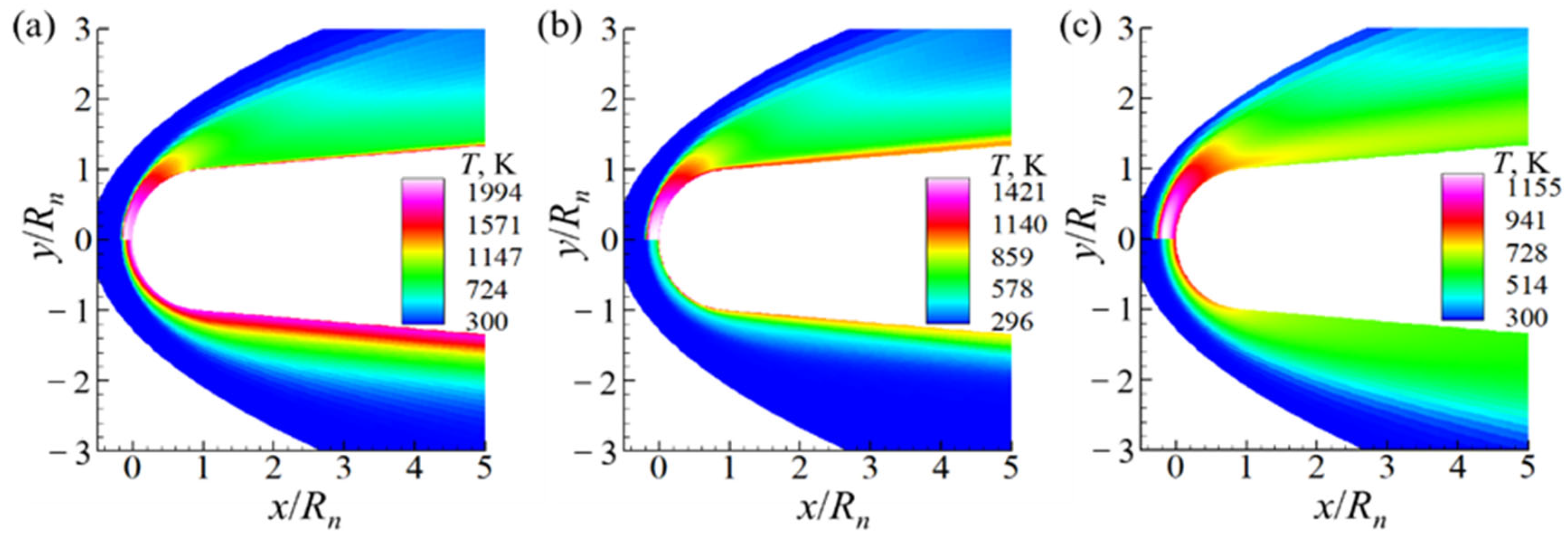
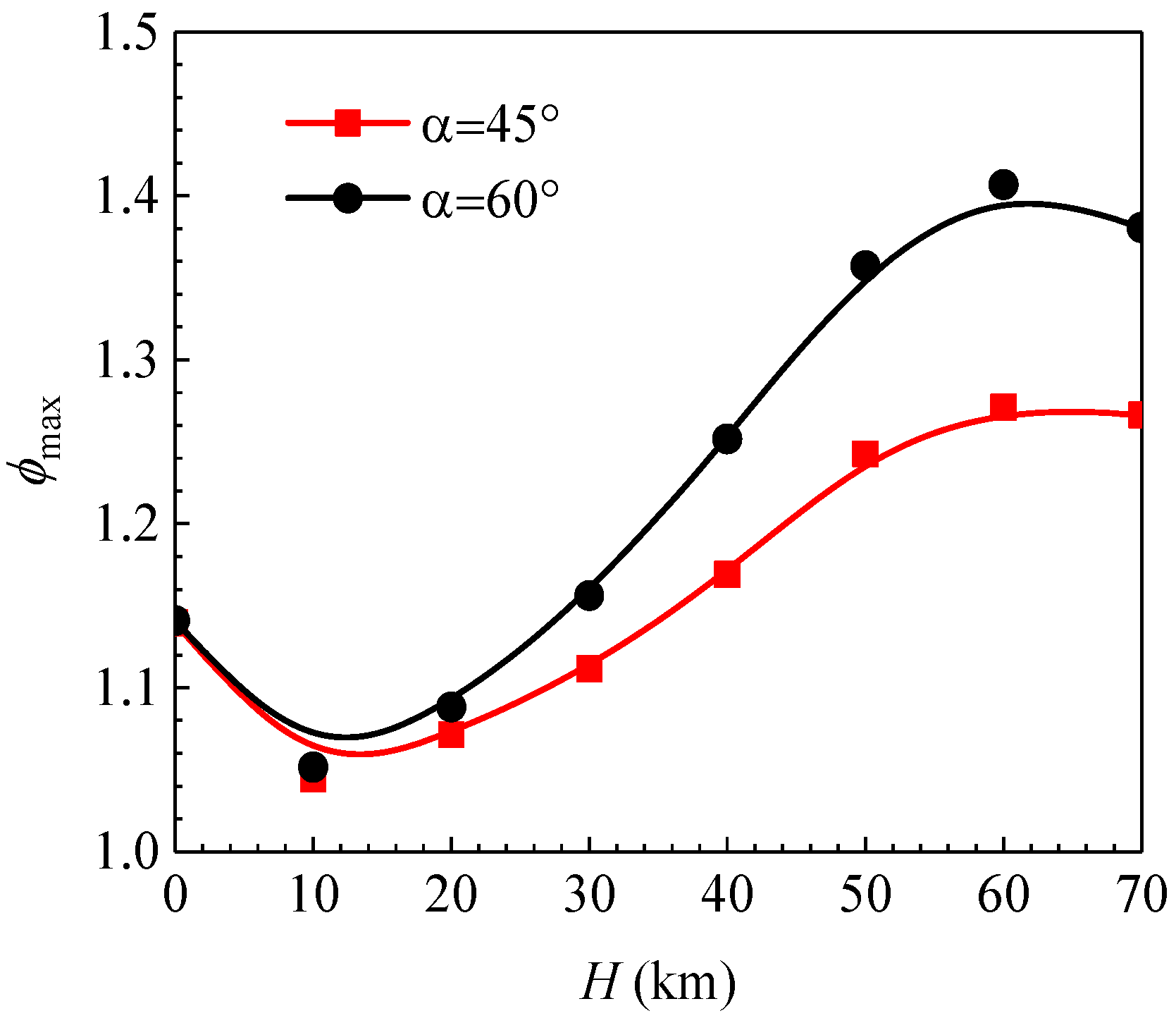
The level and distribution of the translational rotation temperature and vibrational electron temperature along the stagnation line varied significantly according to the altitude. The translational rotation temperature was higher than the vibration selection temperature, and the thickness of the separated shock wave was different under the two temperature modes. The degree of thermal imbalance increased with the altitude. At α = 60°, the maximum thermal nonequilibrium degree was 1.4, which is higher than 1.25 at α = 45°.
(2)
The reaction heat release at α = 60° was higher than that at α = 45°. The reaction heat decreased with increasing altitude. At low altitudes, the NO concentration along the hysteresis line was more than three orders of magnitude higher than that at high altitudes.
(3)
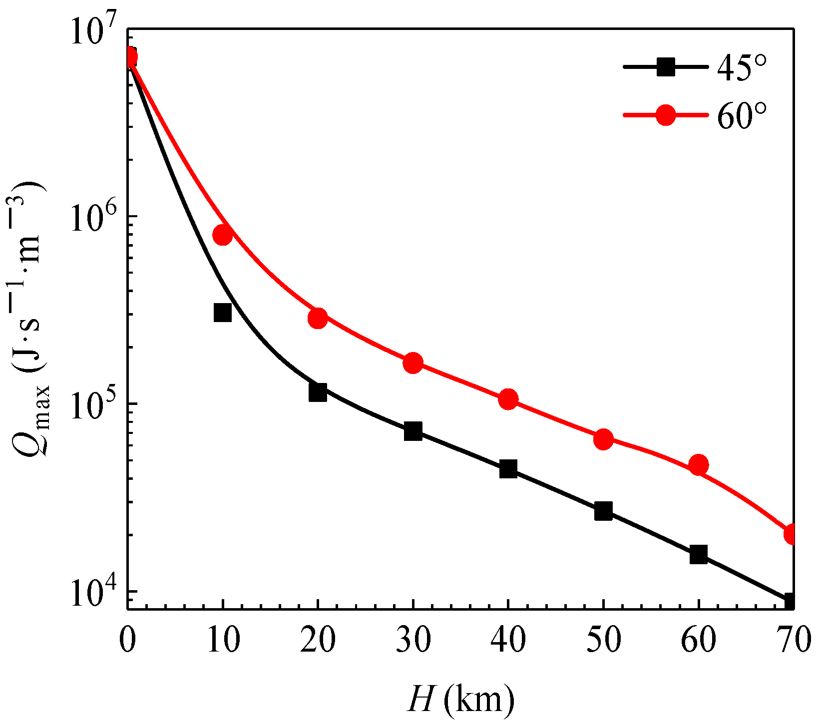
At the two launch angles, the magnitude of the maximum heat flux decreased sharply. The heat flux dropped sharply from 7 MW/m2 at H = 0 km to approximately 2 MW/m2 at H = 70 km. In addition, the maximum heat flux at α = 60° was higher than that at α = 45°. The heat flux was approximately twice as high as that at an altitude of 20 km. The wall temperature distribution was similar to that of the heat flux distribution, and the surface temperature decreased less rapidly than did the heat flux.

Author Contributions

Investigation, W.G.; methodology, S.D.; validation, W.G.; writing—original draft preparation, P.Z.; writing—review and editing, Q.N.; supervision, Q.N.; funding acquisition, Q.N. All authors have read and agreed to the published version of the manuscript.

Funding

This research was funded by the National Nature Science Foundation of China, grant number U22B2045.

Data Availability Statement

Not applicable.

Acknowledgments

The authors gratefully thank the anonymous reviewers for their constructive comments for improving the presentation. All authors have agreed to the listing of authors.

Conflicts of Interest

The authors declare no conflict of interest.

References

  1. Lunan, D.A. Waverider, A Revised Chronology. In Proceedings of the 20th AIAA International Space Planes and Hypersonic Systems and Technologies Conference, Glasgow, Scotland, 6–9 July 2015. [Google Scholar]
  2. Fair, H. Advances in electromagnetic launch science and technology and its applications. IEEE Trans. Magn. 2009, 45, 225–230. [Google Scholar] [CrossRef]
  3. Wang, X.; Li, Y.; Shi, Z.; Cao, B.; Cao, Y.; Zhao, H.; Gong, X. Research on Vehicle-Mounted Electromagnetic Ejection Remote Fire Extinguishing System. Math. Probl. Eng. 2022, 2022, 2129942. [Google Scholar] [CrossRef]
  4. Ma, W.; Lu, J.; Liu, Y. Research progress of electromagnetic launch technology. IEEE Trans. Plasma Sci. 2019, 47, 2197–2205. [Google Scholar] [CrossRef]
  5. Dumm, J.; Murray, K. Electromagnetic propulsion systems: Multipurpose platforms of the future. In Proceedings of the Ninth Annual Freshman Conference, Pittsburgh, PA, USA, 4 April 2009. [Google Scholar]
  6. Miró, F.M.; Beyak, E.S.; Mullen, D.; Pinna, F.; Reed, H.L. Ionization and dissociation effects on hypersonic boundary-layer stability. In Proceedings of the 31st Congress of the International Council of the Aeronautical Sciences, Belo Horizonte, Brazil, 9–14 September 2018. [Google Scholar]
  7. Si, W.; Huang, G.; Zhu, Y.; Chen, S.; Lee, C. Hypersonic aerodynamic heating over a flared cone with wavy wall. Phys. Fluids 2019, 31, 051702. [Google Scholar]
  8. Yazdani, N.M.; Olyaei, M.H. Optimization of Electromagnetic Railgun and Projectile’s Trajectory by Genetic Algorithm. Majlesi J. Telecommun. Devices 2022, 11, 27–32. [Google Scholar] [CrossRef]
  9. Fair, H.D. Progress in electromagnetic launch science and technology. IEEE Trans. Magn. 2006, 43, 93–98. [Google Scholar] [CrossRef]
  10. Shen, J.; Fan, S.; Ji, Y.; Zhu, Q.; Duan, J. Aerodynamics analysis of a hypersonic electromagnetic gun launched projectile. Def. Technol. 2020, 16, 753–761. [Google Scholar] [CrossRef]
  11. Kasahara, H.; Matsuo, A. The effect of shape on the aerodynamic and thermal performance of hypersonic projectiles launched by a ground-based railgun. In Proceedings of the 2018 AIAA Aerospace Sciences Meeting, Kissimmee, FL, USA, 8–12 January 2018. [Google Scholar]
  12. Rahman, F.; Srinivas, G. Aerodynamic performance enhancement of electromagnetic gun projectile using numerical techniques. J. Adv. Res. Fluid Mech. Therm. Sci. 2021, 80, 136–152. [Google Scholar] [CrossRef]
  13. Justus, C.G. The NASA/MSFC Global Reference Atmospheric Model_1995 Version (GRAM-95); National Aeronautics and Space Administration, Marshall Space Flight Center: Alabama, AL, USA, 1995.
  14. Sarma, G. Physico–chemical modelling in hypersonic flow simulation. Prog. Aerosp. Sci. 2000, 36, 281–349. [Google Scholar] [CrossRef]
  15. Niu, Q.; Yuan, Z.; Dong, S.; Tan, H. Assessment of nonequilibrium air-chemistry models on species formation in hypersonic shock layer. Int. J. Heat Mass Transf. 2018, 127, 703–716. [Google Scholar] [CrossRef]
  16. Gnoffo, P.A.; Cheatwood, F.M. User’s Manual for the Langley Aerothermodynamic Upwind Relaxation Algorithm (LAURA); National Aeronautics and Space Administration, Langley Research Center: Hampton, VA, USA, 1996.
  17. Park, C. Nonequilibrium Hypersonic Aerothermodynamics; Wiley-Interscience: Hoboken, NJ, USA, 1989. [Google Scholar]
  18. Dutton, F.B. Dalton’s law of partial pressures. J. Chem. Educ. 1961, 38, A545. [Google Scholar] [CrossRef]
  19. Millikan, R.C.; White, D.R. Systematics of vibrational relaxation. J. Chem. Phys. 1963, 39, 3209–3213. [Google Scholar] [CrossRef]
  20. Gupta, R.N.; Yos, J.M.; Thompson, R.A.; Lee, K.-P. A Review of Reaction Rates and Thermodynamic and Transport Properties for an 11-Species Air Model for Chemical and Thermal Nonequilibrium Calculations to 30,000 K; National Aeronautics and Space Administration, Marshall Space Flight Center: Alabama, AL, USA, 1990.
  21. Lees, L. Hypersonic flow. J. Spacecr. Rocket. 2003, 40, 700–735. [Google Scholar] [CrossRef]
  22. Hayes, W. Hypersonic Flow Theory; Elsevier: Amsterdam, The Netherlands, 2012. [Google Scholar]
  23. Logan, S. The origin and status of the Arrhenius equation. J. Chem. Educ. 1982, 59, 279. [Google Scholar] [CrossRef]
  24. Park, C. Review of chemical-kinetic problems of future NASA missions. I-Earth entries. J. Thermophys. Heat Transf. 1993, 7, 385–398. [Google Scholar] [CrossRef]
  25. Myong, H.K.; Kasagi, N. A new approach to the improvement of k-ε turbulence model for wall-bounded shear flows. JSME Int. J. Ser 2 Fluids Eng. Heat Transf. Power Combust. Thermophys. Prop. 1990, 33, 63–72. [Google Scholar] [CrossRef]
  26. Bertolazzi, E.; Manzini, G. A triangle-based unstructured finite-volume method for chemically reactive hypersonic flows. J. Comput. Phys. 2001, 166, 84–115. [Google Scholar] [CrossRef]
  27. Yee, H.C. On Symmetric and Upwind TVD Schemes; Technical Memorandum 86842; National Aeronautics and Space Administration, Marshall Space Flight Center: Alabama, AL, USA, 1985.
  28. Harten, A. High resolution schemes for hyperbolic conservation laws. J. Comput. Phys. 1997, 49, 357–393. [Google Scholar] [CrossRef]
  29. Blazek, J. Computational Fluid Dynamics: Principles and Applications; Joe-Hayton: Sankt Augustin, Germany, 2015. [Google Scholar]
  30. Adamov, N.P.; Vasenev, L.G.; Zvegintsev, V.I.; Mazhul, I.I.; Nalivaichenko, D.G.; Novikov, A.V.; Kharitonov, A.M.; Shpak, S.I. Characteristics of the AT-303 hypersonic wind tunnel. Part 2. Aerodynamics of the HB-2 reference model. Thermophys. Aeromech. 2006, 13, 157–171. [Google Scholar] [CrossRef]
  31. Tissera, S. Assessment of High-Resolution Methods in Hypersonic Real-Gas Flows. Ph.D. Thesis, Cranfield University, Bedford, UK, 2010. [Google Scholar]
  32. Luo, H.; Kulakhmetov, M.; Alexeenko, A. Ab initio state-specific N2 + O dissociation and exchange modeling for molecular simulations. J. Chem. Phys. 2017, 146, 074303. [Google Scholar] [CrossRef] [PubMed]
  33. Andrienko, D.; Boyd, I.D. Simulation of O2-N Collisions on ab-initio Potential Energy Surfaces. In Proceedings of the 54th AIAA Aerospace Sciences Meeting, San Diego, CA, USA, 4–8 January 2016. [Google Scholar]
Figure 1. Hypersonic projectile fired by an electromagnetic railgun.
Energies 16 01740 g001
Figure 2. Geometry size and grid of HB-2 test model.
Energies 16 01740 g002
Figure 3. Comparison of surface properties between computational and experimental data [30].
Energies 16 01740 g003
Figure 4. Comparison of flow parameters along the stagnation line between computational and reference data [31].
Energies 16 01740 g004
Figure 5. Computational domain and grid of blunt body.
Energies 16 01740 g005
Figure 6. Contours of translational–rotational temperature and vibration–electron temperature at (a) 10 km, (b) 30 km, and (c) 60 km.
Energies 16 01740 g006
Figure 7. Temperature curves along the stagnation line at α = 60°.
Energies 16 01740 g007
Figure 8. Maximum thermal nonequilibrium effect for α = 45° and α = 60° cases.
Energies 16 01740 g008
Figure 9. Mole faction of NO along the stagnation line.
Energies 16 01740 g009
Figure 10. Reaction heat release along the stagnation line.
Energies 16 01740 g010
Figure 11. Heat flux profiles of blunt body surface in representative cases.
Energies 16 01740 g011
Figure 12. Maximum heat flux of surface with altitudes in two launching angles.
Energies 16 01740 g012
Figure 13. Surface temperature profiles of blunt body for representative cases.
Energies 16 01740 g013
Figure 14. Maximum surface temperature with altitudes in two launching angles.
Energies 16 01740 g014
Table 1. Forward reaction rate coefficients in air-chemistry models (cm3/mole/s).
ReactionPark 93
N2 + M1 → N + N + M13.0 × 1022 T−1.6 exp(−1.132 × 10⁵/T)
O2 + M2 → O + O + M22.0 × 1021 T−1.5 exp(−5.95 × 10⁴/T)
NO + M3 → N + O + M35.0 × 1015 exp(−7.55 × 10⁴/T)
N2 + O → NO + N6.4 × 1017 T−1.0 exp(−3.84 × 10⁴/T)
NO + O → O2 + N8.4 × 1012 exp(−1.945 × 10⁴/T)
N + O → NO+ + e-8.8 × 10⁸ T1.0 exp(−3.19 × 10⁴/T)
N2 + e- → N + N + e-1.2 × 1025
Table 2. Weight factors of the controlling temperature.
ReactionForwardBackward
abab
Dissociation0.50.51.00.0
Neutral exchange1.00.01.00.0
Associative ionization1.00.00.01.0
Charge exchange1.00.01.00.0
Electron impact dissociation0.01.00.50.5
Table 3. Free stream conditions at representative altitudes.
H, kmρ, kg/m3T, KP, PaU,45°, m/sU,60°, m/s
01.2250288101,32530003000
100.413522326,50017372041
200.0725216552915001741
300.0184226119714091637
400.004025028713251575
500.00102717912361505
600.00032472211681450
700.0000672205.210991350
Disclaimer/Publisher’s Note: The statements, opinions and data contained in all publications are solely those of the individual author(s) and contributor(s) and not of MDPI and/or the editor(s). MDPI and/or the editor(s) disclaim responsibility for any injury to people or property resulting from any ideas, methods, instructions or products referred to in the content.

