Application of the Temperature Oscillation Method to Laminar Flow in Straight Horizontal and Curved Minichannels

Abstract

This work deals with the application of the temperature oscillation method to measure local values of the heat transfer coefficient in laminar flow in a straight horizontal pipe and in a pipe with a bend. This method, applied here for the first time in such experimental conditions, uses a time-varying heat flux as a boundary condition, which is a condition of the third kind. Since an analytical solution for such conditions could not be identified in the existing literature, a numerical study of this problem is applied here. Experimental data for a straight horizontal pipe confirm the numerical results within a reasonable level of error. Experimental measurements on a straight horizontal tube are consistent with predicted results in the literature for both total and local heat transfer coefficient values. The measurements on bent tubes show a very significant influence on the local values compared to the straight tube and in the overall values this change appears as an increase in the heat transfer coefficient.

1. Introduction

One of the most commonly used devices in process engineering is the heat exchanger, a device used to transfer heat between a hot and a cold fluid in order to preheat or cool process streams. However, heat exchangers are also integral part of other apparatuses, such as chemical reactors, to remove the reaction heat of exothermic processes. Heat exchangers in process industry are most often designed as convective heat exchangers, where a solid wall separates two flowing media at different temperatures. The basic equation for calculating heat transfer using convection is Newton’s law of cooling:

$$\dot{Q}=hS\Delta T$$

(1)

where h represents the heat transfer coefficient, S the heat transfer area and $\Delta T$ the temperature difference between the very distant fluid and the surface temperature of the wall. $\dot{Q}$ represents the heat power that was transferred in the exchanger and is usually the basic parameter when designing a heat exchanger. The temperature difference is usually also entered in process engineering as a process condition (maximum wall temperature due to material degradation, etc.). Thus, the engineering task usually leads to the determination and calculation of the heat transfer coefficient and the necessary heat transfer area.

Over the last decades, academia and industry developed apparatus which contains microstructures to intensify the transfer of heat and mass. Such microstructured equipment is used in process industry as compact heat exchanger or as chemical reactor (see Schubert et al. [1] or Jensen [2]). Several microstructured designs are proposed which have been recently reviewed by Naqiuddin et al. [3]. The equipment itself is usually formed by a system of parallel flow channels in the millimeter and submillimeter range [4]. In consequence of the small size, such devices operate usually in the laminar regime in contrast to the conventional devices.

In the literature we can find a relatively large number of papers on the topic of heat transfer in similar geometries and even in multiphase flows, so it is clear that there is considerable interest in this topic. Zhang et al. [5] have experimentally measured the values of the heat transfer coefficient on the wall of square and rectangular microchannels during the flow of a liquid–gas mixture. They used the heat balance of the system with heating to determine the heat transfer while observing the shape and velocity of the interfacial interface in the transparent channel. Li and Hrnjak [6] prepared an analytical model to predict the heat transfer and pressure drop in two-phase flow in the interstitial ring, which is one of the special flows in liquid–gas mixtures. Huang and Thome [7] experimentally measured heat transfer during boiling of refrigerants in rectangular mini-channels at the scale of micro-electronics heat sinks.

Today, the heat transfer coefficient is most often calculated using numerical simulations (see [8,9]) or experimental measurements. Although numerical simulation is faster and can be significantly cheaper compared to the experiment, it is still necessary to verify the numerical results using experiments, so measuring the heat transfer coefficient is still a topical issue.

The heat transfer coefficient depends on many quantities (thermophysical properties of the fluid, flow regime, solid wall shape, wall surface treatment, direction and size of the local velocity, etc.) and so its determination is relatively difficult. Over the years, many methods and procedures have emerged to determine this coefficient (whether local or average).

Static methods are based on Newton’s law of cooling (Equation (1)) and, with knowledge of the heat transfer surface S, allow direct measurement of the heat transfer coefficient h (either by fixing the temperature difference and measuring the heat output or vice versa). Static methods are very accurate, but very time consuming (until thermal equilibrium of the system is achieved) and require very precise temperature measurements and perfect thermal insulation of the experiment.

Kupčík [10] prepared an experiment measuring the heat transfer coefficient on the wall and bottom of a cylindrical vessel with a mixer (various types). For his measurements, he used thermally insulated vessels with a constant temperature (provided by a thermostat) and determined heat losses to the surroundings of 1–2%, so these were neglected. The vessel walls and bottom were heated with an electrical resistance wire of known power and after the system stabilized, the temperatures of the liquid and of the vessel walls as well as the power in the thermostat, which maintained a constant temperature, were read.

Han and Park [11] prepared experimental measurements of local values of the heat transfer coefficient in a square channel with and without ribbing on the wall. The channel model was created with plexiglass, on which was a very thin stainless steel foil heater. The experiment also contained a total of 90 thermometers to obtain local coefficient values. The authors calculated the deviation of this measurement to 8%. However, when comparing the experimental results with the well-known Dittus Boelter correlation, they found deviations of 5–15%.

Wiberg and Lior [12] measured the heat transfer between the finite size cylinder and the flowing air using a static method and thermochromic crystals (TLCs). The cylinder was made of polystyrene for its very small heat conduction coefficient (and thus a very high Biott number) and minimal heat loss to the cylinder. They applied a heater film with a TLC layer on its surface. The electrical input to the heater was recorded and after stabilizing the thermodynamic equilibrium, the object was photographed by a camera. The local cylinder surface temperature was then subtracted from the TLC calibration curve. The heat transfer coefficient was calculated from the temperature difference and the power dissipation in the heater film.

Ingole and Sundaram [13] used a very similar method to measure the heat transfer between a flat plate and an inclined impinging air jet. However, they did not use TLC for the measurement, but an IR temperature sensor, which was moved to different positions to obtain local values of the heat transfer coefficient.

Dynamic methods of measuring the heat transfer coefficient are based on monitoring the system’s response to a sudden change (usually a change in heat flux). These methods are very fast and efficient, but they require more expensive measurement techniques and very accurate time synchronization of signals. In general, they are less accurate than static methods, but they allow large amounts of data to be measured in a very short time and do not require the system to stabilize in thermodynamic equilibrium.

Debab et al. [14] measured the overall values of the heat transfer coefficient in an agitated reactor with non-Newtonian type of fluid. The cylindrical vessel was equipped with a duplicator with flowing water and from the temperature records (four temperatures in total) the coefficient was calculated according to a relatively simple equation:

$$\overline{h}=\frac{m{c}_p}{S\Delta T}\frac{\mathrm{d}T}{\mathrm{d}t}.$$

(2)

The measuring system is therefore based on monitoring the temperature change in the batch based on the change in water temperature in the duplicator jacket.

Nebuchinov et al. [15] as well as Jainski et al. [16] and others dealt with a very interesting dynamic and optical method. By combining two methods—particle image velocimetry and planar laser induced fluorescence—they were able to monitor the velocity and temperature fields in their experiments and to determine the thickness of the boundary layer and thus calculate local values of the heat transfer coefficient. The stated inaccuracy of temperature measurement was below 5% and the velocity field even below 2%.

Other dynamic methods are, for example, based on 1D semi-infinity body derivation, where it is possible to fix boundary conditions. Yi et al. [17] used this method to cool a very hot plate using an impinging air jet and used thermographic phosphorus to measure the surface temperature of the plate.

There are other specific methods with an oscillating change of one of the parameters, but we discuss these methods in Section 2.

Comparative methods are based on the measurement of another transfer phenomenon (most often mass transfer) and are then converted to heat transfer coefficients by analogy between heat and mass transfer. These are very interesting methods that offer different measurement speeds as well as different measurement accuracies.

Probably the best known comparative method is the electro-diffusion method; Cudak and Karcz [18] used this to measure the heat transfer between the wall and the bottom of an agitated cylindrical vessel. The method is based on measuring the electric current between the anode and cathode in a conductive environment. The magnitude of the measured current is proportional to the magnitude of the mass transfer coefficient. If we use more than one measuring probe, we can also measure local values.

An interesting work was Nusselt [19], which calculated the convective coefficient based on the rate of combustion of coal in an oxygen stream. The measured burnt coal losses were used to calculate the combustion rate and led to the determination of the convective coefficient. The dependence of the convective coefficient and the ambient oxygen velocity proved to be very similar to the literature and so it was confirmed that it is possible to determine the heat transfer coefficients using the measured mass transfer coefficient.

In the literature, we can find a large number of simulation works on the topic of heat transfer, whether it is a multidimensional heat conduction problem or just convective transfer. Although simulations are already of very high quality today, numerical models still require experimental verification.

We can also find a lot of very interesting articles on heat transfer measurements in nanofluids [20] or porous media [21] and so we can judge that this topic is still valid and of interest.

It is not usual in the literature to state the values of the heat transfer coefficient directly. Usually, we encounter its dimensionless value in the form of a Nusselt number:

$$\mathrm{Nu}=\frac{h{L}_{CH}}{k}.$$

(3)

The dimensionless value has the great benefit that the dependences of the Nusselt number are the same for all geometrically similar systems. The Nusselt number is then used to relate to Reynolds number:

$$\mathrm{Re}=\frac{\overline{u}{D}_H}{\nu }=\frac{\overline{u}{D}_H\varrho }{\mu }$$

(4)

and Prandtl number:

$$\mathrm{Pr}=\frac{\nu }{a}=\frac{k}{\varrho c_p}$$

(5)

to a typical power dependence:

$$\mathrm{Nu}=C{\mathrm{Re}}^m{\mathrm{Pr}}^n.$$

(6)

C represents the geometric constant of the experiment and m and n are the exponents of the Reynolds and Prandt numbers. The typical exponent values for the Prandtl number are 1/3 for cooling or 0.4 for heating of the fluid and the typical exponent values for the Reynolds number are 1/2 and 1/3 for laminar flow and 2/3 to 4/5 for turbulent flow.

Laminar flow can appear in geometries (with other conditions being equal) with very small dimensions of the flow cross-section. Typically, when cooling water, in a tube with an internal diameter of $d_i=1$ mm, we encounter a laminar flow even for an average volume velocity of $\overline{u}=2$ m/s.

When studying heat transfer in laminar flow in a pipe, we come across two basic boundary conditions, namely the condition of the first type $T=\mathrm{const}.$ (represents heat transfer during a phase change, which is isothermal) and a condition of the second kind $q=\mathrm{const}.$ (represents the condition of heating the pipe by passing an electric current). For these two basic conditions, relations are derived for local and average values of the heat transfer coefficient (resp. Nusselt numbers).

At the same time, in laminar flow, the shape of the velocity profile that enters the measuring section of the pipe is very important (especially whether it is hydrodynamically developed). In our experiments, we limited ourselves only to measurements with a hydrodynamically developed velocity profile, so it is not necessary to list the relations valid for the newly developing velocity profile. In the publication Heat Atlas [22], we can find

$${\mathrm{Nu}}_{x,T}=1.077{\left[\mathrm{Re}\mathrm{Pr}(d_i/x)\right]}^{1/3}$$

(7)

at the entrance of the measuring section where the temperature profile begins to develop and

$${\mathrm{Nu}}_{x,T}=3.66$$

(8)

for very distant measurement points of the tube, where the temperature and velocity profile is already stable. We can also find very similar dependencies for the boundary condition of the second kind

$${\mathrm{Nu}}_{x,T}=1.302{\left[\mathrm{Re}\mathrm{Pr}(d_i/x)\right]}^{1/3}$$

(9)

at the entrance of the measuring section where the temperature profile begins to develop and

$${\mathrm{Nu}}_{x,T}=4.354$$

(10)

for very distant measurement points of the tube, where the temperature and velocity profiles are already stable.

We can also find correlations for the average values of the Nusselt numbers for both boundary conditions

$${\overline{\mathrm{Nu}}}_T=1.615{\left[\mathrm{Re}\mathrm{Pr}(d_i/L)\right]}^{1/3}$$

(11)

and

$${\overline{\mathrm{Nu}}}_q=1.953{\left[\mathrm{Re}\mathrm{Pr}(d_i/L)\right]}^{1/3}.$$

(12)

The method we used (temperature oscillation method) does not satisfy even one of the mentioned boundary conditions (it uses a boundary condition of the third kind—Cauchy’s), so in this article we investigate this problem numerically and experimentally.

This paper deals with the application of the dynamic method of temperature oscillations for the measurement of local heat transfer coefficient values in straight and curved tubes. Straight and bent pipes are a very common engineering problem in the design of heat exchangers. Very small tubes can provide a relatively large heat transfer area at a very small place and offer large heat outputs at the same time. A simulation of this problem with a non-standard boundary condition is prepared before measurements and numerical results are verified experimentally. Further measurements are focused on the effect of pipe bending and the change of both local and overall values of the heat transfer coefficient and Nusselt number. Pressure losses for the determination of thermal enhancement factors were not monitored.

2. Temperature Oscillation Method

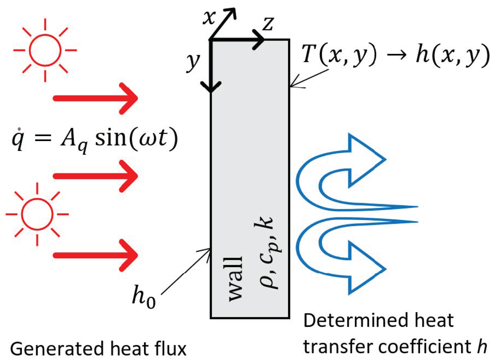
The temperature oscillation method is a dynamic method of measuring local values of the heat transfer coefficient. The method determines this coefficient by sensing the surface temperature (in our case by an IR camera) in time, which is affected by a periodical change in the magnitude of the generated heat flux (we use radiative heat flux). A certain delay can be found between the transmitted heat flux signal and the surface temperature record, which is directly related to the value of the heat transfer coefficient on the reverse side of the wall. A simplified scheme of the thermal oscillation method can be seen in Figure 1.

The method assumes a homogeneous wall of relatively high conductivity (generally metallic materials) with a thickness in the order of millimeters so that there is no excessive thermal resistance and the body does not begin to behave as semi-infinite. In this case, the time-temperature dependence in the body can be described using the Fourier equation and if we neglect the effect of lateral conduction in the plate (the first two partial derivatives on the right side of the equation) we obtain:

$$\frac{\partial T}{\partial t}=a\left(\underset{=0}{\underbrace{\frac{{\partial }^{2}T}{\partial x^2}+\frac{{\partial }^{2}T}{\partial y^2}}}+\frac{{\partial }^{2}T}{\partial z^2}\right)=\frac{k}{\varrho c_p}\frac{{\partial }^{2}T}{\partial z^2}$$

(13)

By adding two boundary and one initial conditions, it is then possible to solve this partial differential equation, on the left side:

$$k{\left.\frac{\partial T}{\partial z}\right|}_{z=0}=A_{q}sin\left(\omega t\right)-h_0{T|}_{z=0}$$

(14)

on the right side:

$$k{\left.\frac{\partial T}{\partial z}\right|}_{z=\max }{=hT|}_{z=\max }$$

(15)

and the initial condition is selected as:

$${T|}_{t=0}=T_0=T_{\mathrm{w}}$$

(16)

The overall derivation of the method has already been mentioned, for example, in Wandelt and Roetzal [23] or in the Ph.D. thesis by Freund [24]. This partial differential equation can be solved analytically using the Laplace transform and leads to the solution

$$T(z,t)=A\left(z\right)sin(\omega t-\phi (z\left)\right)$$

(17)

where $\phi$ is the phase delay between the two signals. This phase delay can be converted into a heat transfer coefficient on the reverse side of the measured wall. In the derivation, there is also a heat transfer coefficient $h_0$, which takes into account the formation of natural convection on the illuminated (heated) side of the wall. It is necessary to know this for a correct calculation; however, the sensitivity analysis of the method shows that the effect of this factor is practically negligible; a much more significant effect is on the thermophysical properties of the wall.

From the same derivation, it is also possible to measure the heat transfer coefficient on the opposite side of the wall using the amplitudes of the temperature signal. Such a measurement requires knowledge of the size of the incident heat flux and a very accurate reading of the surface temperature. This measurement was not used in this work.

The original idea of the possibility of measuring the heat transfer coefficient using thermal oscillations was from Hausen in the 1930s. This idea was then further studied by his students, such as Glaser [25], Langhans [26], Kast [27], Stang and Bush [28] and also Roetzel [29]. Another author was Freund at the beginning of the new millennium ([24,30,31]) and then our research team ([32,33,34]).

The method proved to be functional for various types of measurements from simple geometries to very complex systems, but it was never used for measuring heat transfer coefficient in laminar flow. For the experiments, we chose a geometry with an inner diameter $d_i=1\mathrm{mm}$ and a measuring zone length $L=80\mathrm{mm}$. In front of the measuring zone, a settling zone with a length of $200\times d_i$ was prepared for the stabilization of the velocity profile and was provided with thermal insulation to guarantee the formation of the temperature profile starting only at the beginning of the measuring zone.

3. Numerical Study

As elaborated in the Introduction, only boundary conditions of the first and second kind are usually studied in laminar flow. We do not see the possibility of an analytical solution for our problem with this type of time-dependent boundary condition and so we have prepared a numerical study of this problem in ANSYS Fluent software.

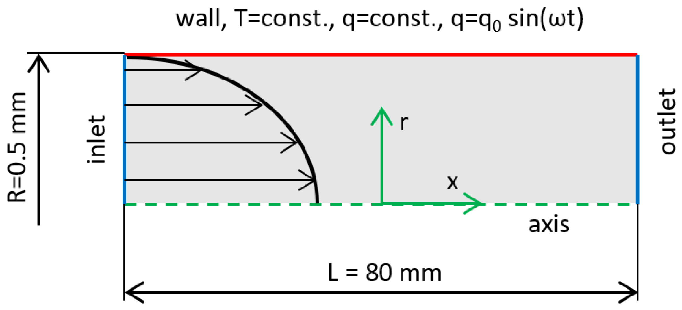
We prepared a 2D axisymmetric geometry that corresponds to the experimental measurement ($d_i=2R=1\mathrm{mm}$ and $L=80\mathrm{mm}$); details and boundary conditions of the numerical solution are shown in Figure 2.

As an input boundary condition, the UDF (used-defined function) of the parabolic velocity profile is chosen, which corresponds to the analytical solution of the pressure-driven flow of a viscous Newtonian fluid in a circular geometry:

$$u_x\left(r\right)=2\overline{u}\left[1-{\left(\frac{r}{R}\right)}^2\right]$$

(18)

$u_x\left(r\right)$ represents the velocity profile along the radial coordinate, $\overline{u}$ the mean volumetric velocity, r the radial coordinate and R the inner radius of the tube. The outlet boundary conditions are set according to

Table 1. Momentum and thermal boundary conditions for numerical calculations. The angular frequency was varied for different calculations. The results are presented for $\omega =0.1047\mathrm{rad}/\mathrm{s}$, corresponding to the period $T=60\mathrm{s}$ (same as in the experiments).

Boundary	Momentum	Thermal
inlet	UDF parabolic	T = 300 K
outlet	pressure outlet	-
wall	stationary, no slip	T = 310 K or q = 25 kW/m2 or q = 25 + 1 sin($\omega t$) kW/m2
axis	axisymetric	axisymetric

and all calculations are set as axisymmetric. For the two basic boundary conditions, the calculation is performed as steady-state and by the SIMPLEC method. Viscous behavior modeling is set to laminar and heat equations are turned on. The thermophysical properties of water were taken from the Fluent database and assumed as constant.

Boundary conditions for calculation are listed in the Table 1.

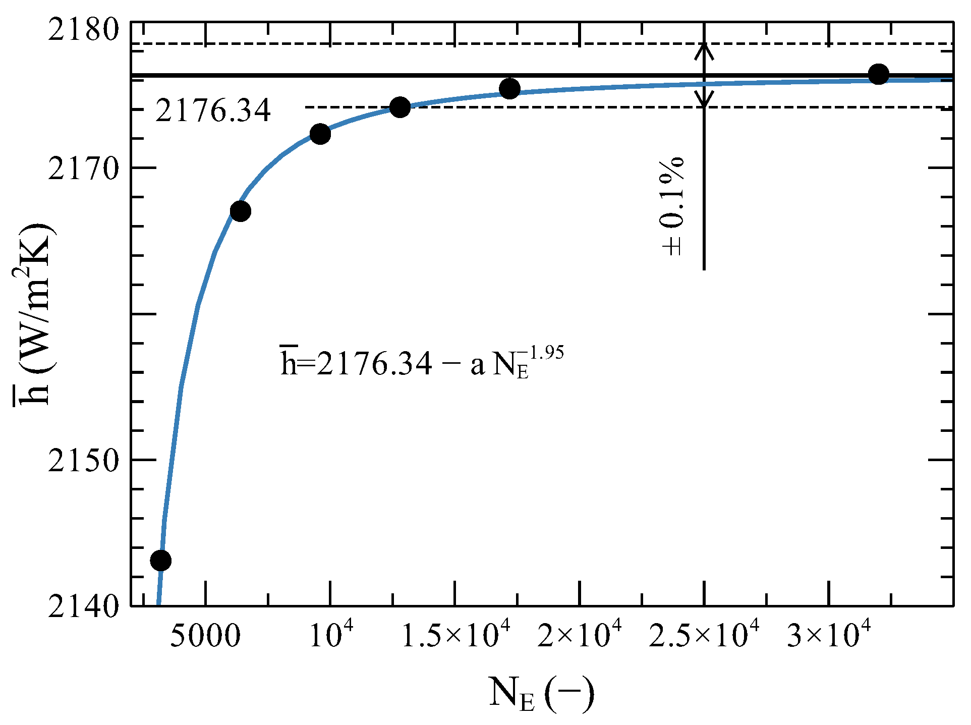
The computational mesh of the task is divided into 320 points along the axis (corresponding to a physical size of 0.25 mm) and a varying number of mesh points in the radial direction. Towards the wall, the mesh was refined with a bias function with a bias setting of 15. The calculation was performed for different mesh densities and the average value of the heat transfer coefficient was monitored as the main parameter. The results of the grid independence study can be seen in Figure 3—this is actually the dependence of the main parameter on the number of mesh elements.

From the results we can see that the computational network with a number of elements greater than 12,000 meets the commonly used condition that the results do not differ by more than 0.1%. However, the task is very simple and the computation times are not long for any computational mesh, so that the finest mesh with the number of elements of 32,000 was chosen.

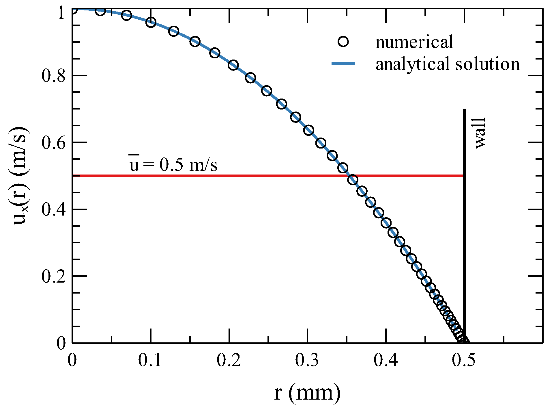
From the numerical solution, the output velocity profile (see Figure 4) was checked to see if it also corresponds to the analytical solution. The input velocity profile is given by the function, so it is not necessary to check it.

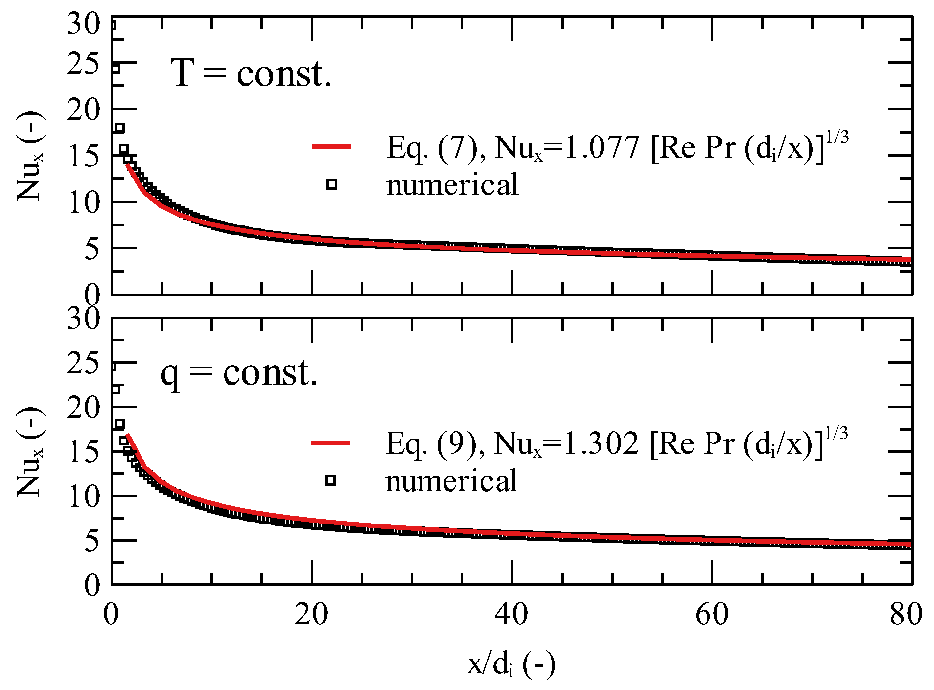
Before the actual calculation with the time-dependent Cauchy boundary condition, calculations were performed with two basic boundary conditions ($T=\mathrm{const}.$ and $q=\mathrm{const}.$) to verify the resulting heat transfer coefficients (resp. Nusselt numbers).

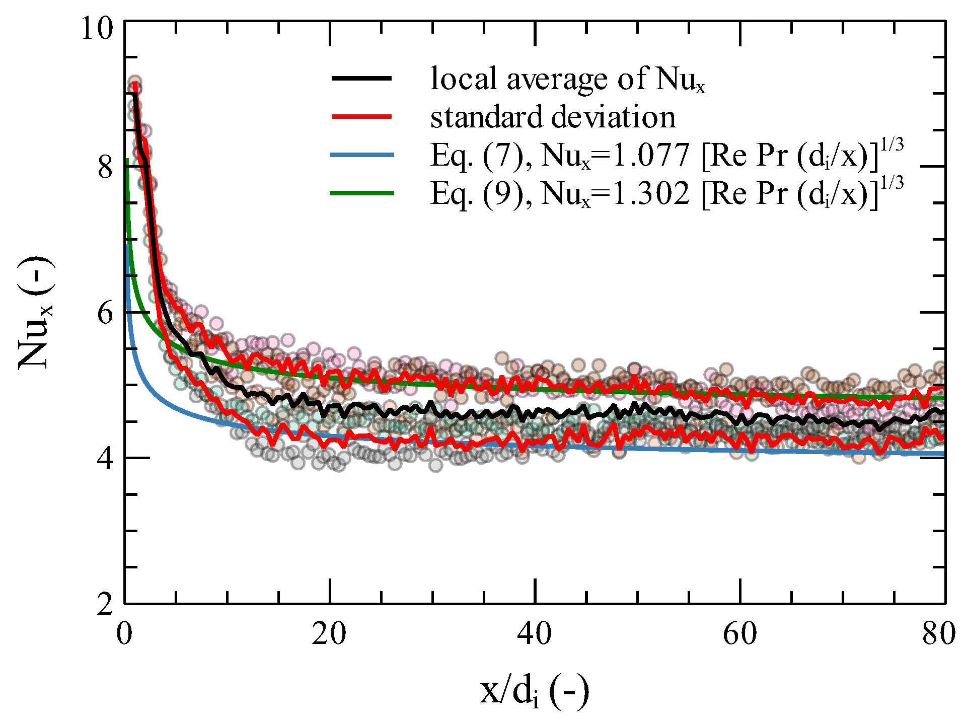
In Figure 5 we can see a comparison of the numerical results of the local values of Nusselt numbers from the beginning of the measuring zone with the analytical solution according to Equations (7) and (9).

From the results, we can judge that the setting of the numerical model is set satisfactorily and the calculation meets both basic boundary conditions. Deviations from the analytical solution are minimal and we consider the results to be sufficient. For further calculations, the solution setting was changed to transient and the boundary condition was changed to

$$q\left(t\right)=q_0+q_{A}sin\left(\omega t\right),$$

(19)

which corresponds to the TOIRT method. The first 2000 iterations were performed without changing the heat flux density; after the calculation of the velocity field in the entire task, the calculation was switched to a new, time-dependent boundary condition.

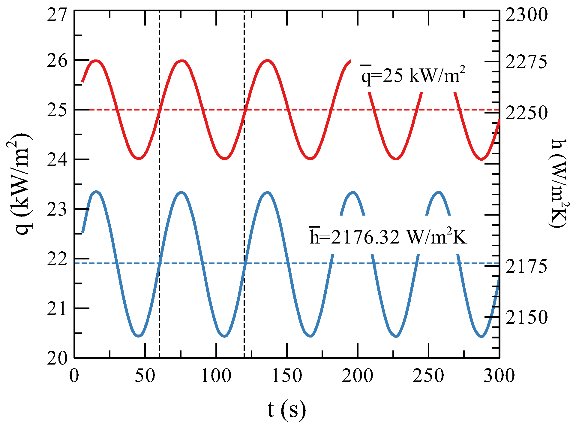
Due to the fact that the heat flux on the wall changes, the heat transfer coefficient also changes partially with the same frequency, so it is necessary to evaluate the time average values of the heat transfer coefficient. A study was conducted on this effect and it was found that if the ratio of the amplitude and the time average value of the heat flow is not greater than 15%, the ratio of the amplitude and time average in the heat transfer coefficient is less than 5%, which we consider an acceptable deviation for time averaging. One of the solutions can be seen in Figure 6.

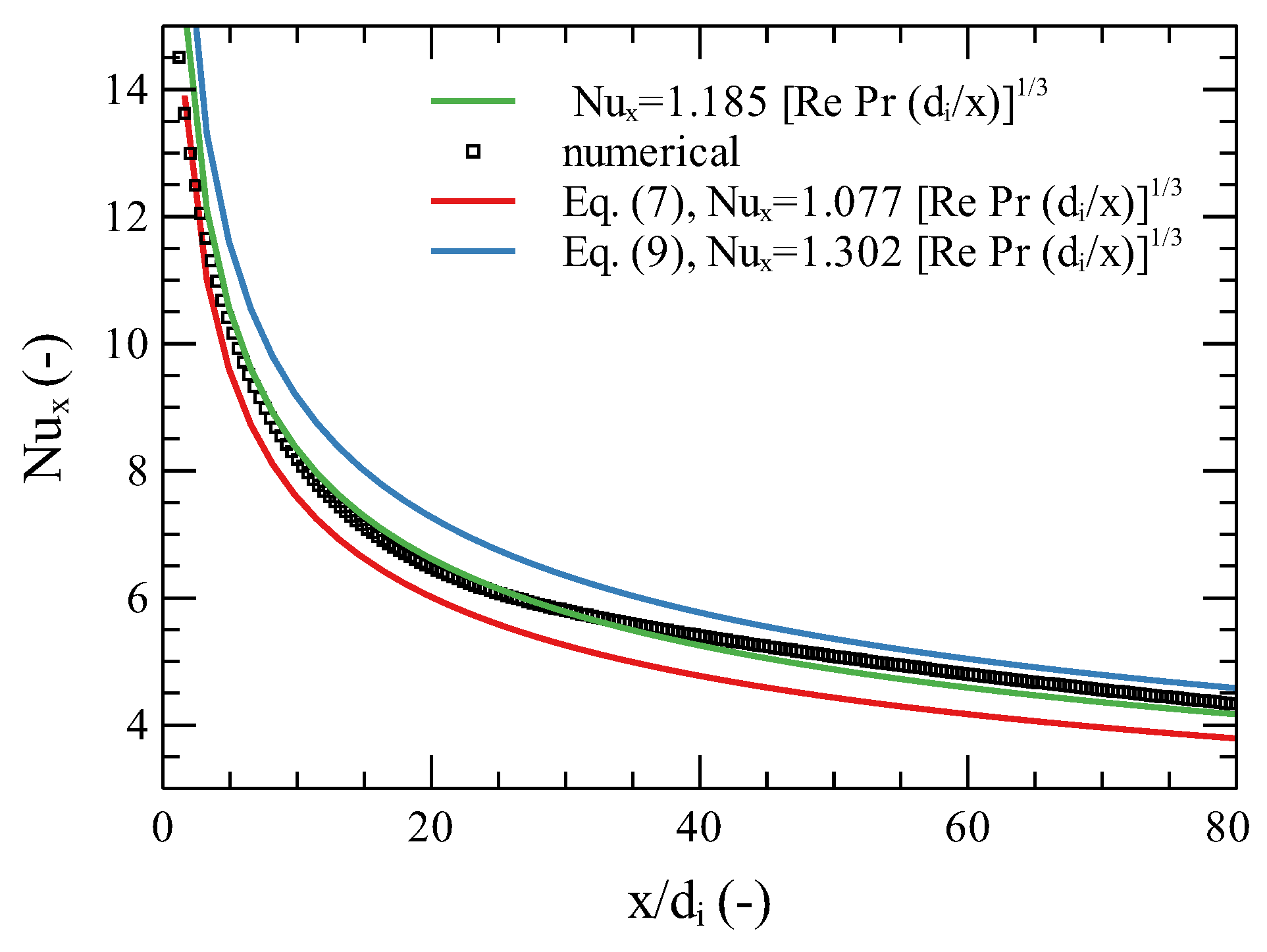
During numerical simulations, no dependence of the shape of the heat transfer coefficient on the amplitude or frequency (or period) of the heat flux signal was discovered. However, the shape of the course of the heat transfer coefficient is slightly different from the shapes for boundary conditions of the first and second type; see Figure 7.

This deviation can result from a change in the heat flux q on the wall of the task, which slightly changes the value of the heat transfer coefficient. The average deviation of the numerically calculated points from the correlation is 1.4%, so we assume that the influence has no major effect on the result.

Although this numerical study is only very simple and certainly does not affect all aspects, we can judge that the time-varying boundary condition slightly changes the profile of the heat transfer coefficient from the entrance of the measuring zone. The results of the numerical study show that with this boundary condition we can expect results approximately in the middle between the two basic boundary conditions. Many more numerical simulations are required for further conclusions.

4. Experiment

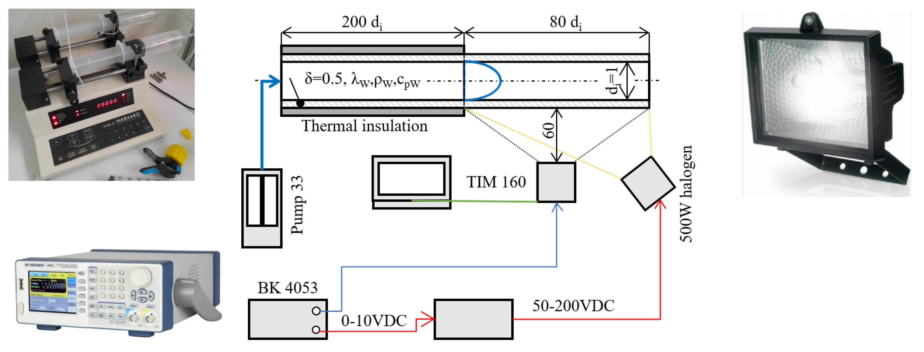
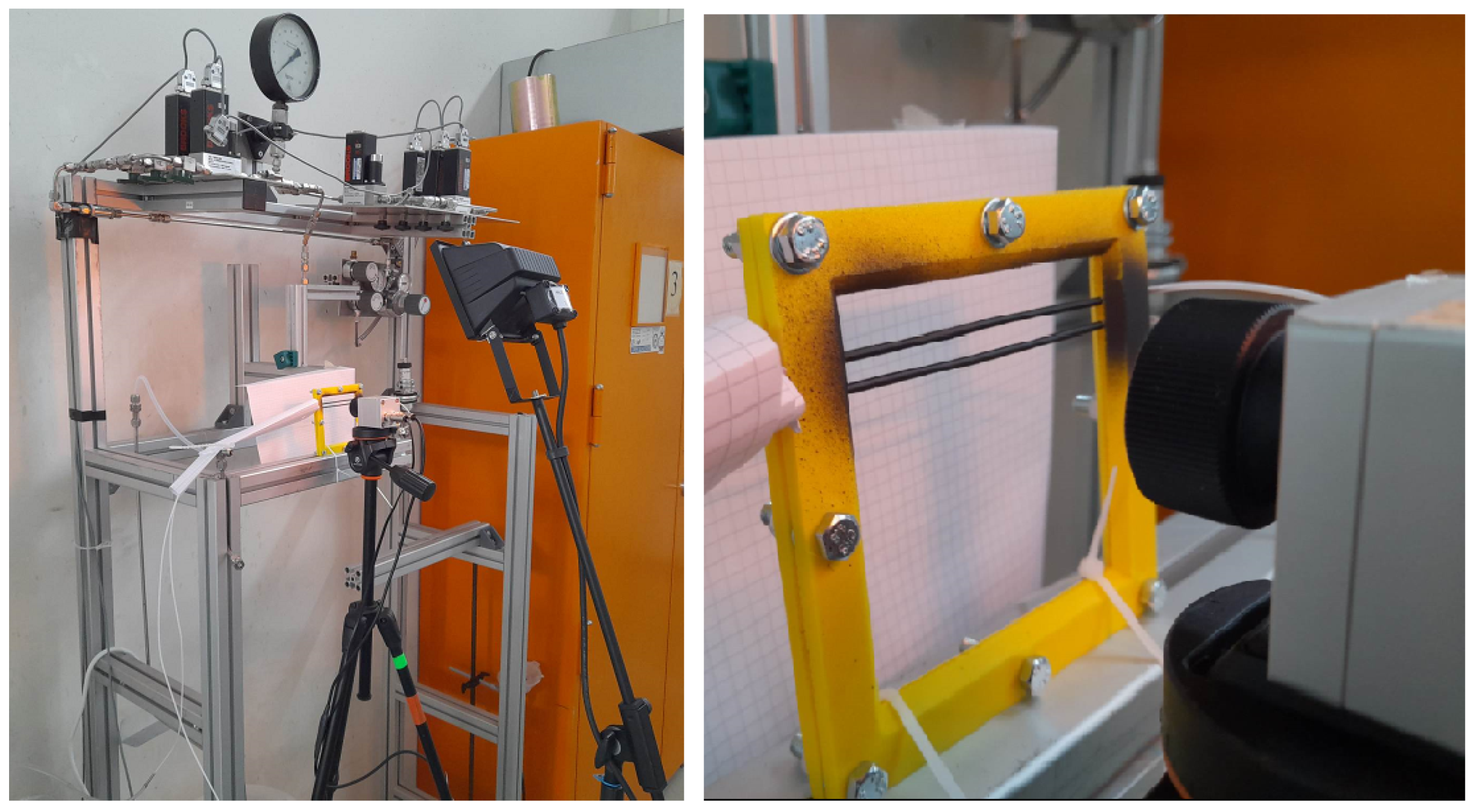
In order to fulfill the prerequisites for the method, especially the perfect synchronization of the signals of the generated sinusoidal heat flux and the timing of the IR camera capture, we used a very precise two-channel laboratory functional source BK 4053 (BK Precision, stated accuracy for our setup 2 ms between channels). In the first channel, we generated a 1–10 V DC sine wave that was sent to voltage sources (1.5 kW max) and they supplied an amplified 50–200 V DC function to the halogen lights. We used 500 W halogen lights due to their very poor efficiency, so most of the supplied energy was converted into heat, sending a radiative heat flux to the wall. The second channel was used to generate a 0–1 V DC step function that controlled the triggering of the IR camera TIM 160 (MicroEpsilon, 46 degrees optics, spatial resolution 160 × 120 points, max scanning frequency 120 Hz, sensitivity 80 mK). The details, photos and connection of the experiment can be seen in Figure 8 and Figure 9.

The poly-tetra-fluoro-ethylene (PTFE) tube was fixed in a prismatic holder and the whole holder was fixed to the structure. In front of the measuring section itself, there is a settling zone for the possibility of developing a velocity profile with a length of $200\times d_i$, but this part was thermally insulated to ensure that the temperature profile starts to form only at the beginning of the measuring zone. Volumetric flow rate of water was provided by two very precise Harvard Pump 33 syringe pumps (measured range is 5–90 mL/min, Re = 100–2000).

One of the most critical parameters is the choice of the period (or angular frequency) of the transmitted heat flux signal. It is chosen based on the equation of dimensionless thickness:

$$\xi =\delta \sqrt{\frac{\omega }{2a_W}}<0.5,$$

(20)

where $\delta$ represents the physical thickness of the wall, $\omega$ the angular velocity of the transmitted heat flux signal and $a_W$ the thermal diffusivity of the wall. Ref. [24] writes that if the dimensionless wall thickness $\xi$ is less than 0.5, the effect of lateral conduction in the wall can be neglected and the whole task can be taken as 1D heat conduction through the wall (prerequisites of the method). The minimum operating signal period results for the PTFE material used (${\rho }_W=2200\mathrm{kg}/{\mathrm{m}}^3$, $k_W=0.23\mathrm{W}/\left(\mathrm{m}\mathrm{K}\right)$ and $c_{pW}=960\mathrm{J}/\left(\mathrm{kg}\mathrm{K}\right)$) and a wall thickness of 0.5 mm is 29 s, we chose a period of 60 s for our experiments.

There is also a certain phase delay of the measuring apparatus itself (mainly the inherent thermal capacity of halogen lamps). This systemic delay must be considered; otherwise, the method evaluates incorrect results. We have already measured the system delay several times with various methods in our previous articles and it is in the order of hundreds of milliseconds (545 ms to be exact).

A thermocouple was installed behind the measuring section to monitor the temperature. This temperature was then used to determine the thermophysical properties of water and subsequent calculations.

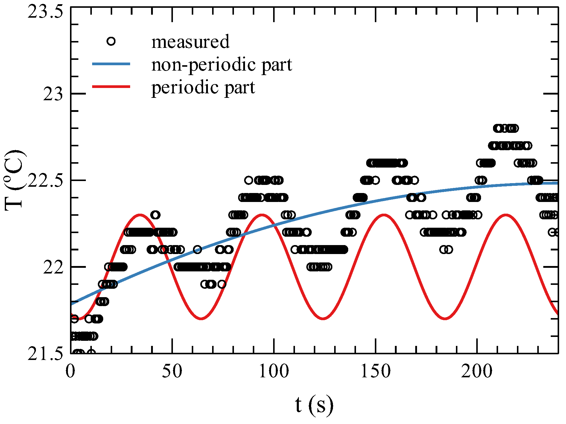
For sensing the surface temperature, we used an IR camera with a frequency of 2 Hz, which is sufficient time resolution for these experiments. The time recording of the surface temperature has two basic components, periodic and non-periodic. The periodic component is the one that is evaluated after the measurement, but first the non-periodic component must be subtracted from the record. The phase is subtracted from the periodic part using non-linear regression or fast Fourier transformation and compared with the phase of the transmitted signal; see Figure 10. The phase difference is then directly related to the heat transfer coefficient.

For the method, it is necessary to know the thermophysical properties of the wall as well as the heat transfer coefficient on the illuminated side, but the sensitivity analysis showed that it is practically negligible (this value is set to $5\mathrm{W}/\left({\mathrm{m}}^2\mathrm{K}\right))$.

For curved tube measurements, the PTFE tube was bent into the desired shape and firmly mounted to the measuring stand. The parts of the pipes that were not part of the measuring section were thermally insulated. Within that article, the change in the heat transfer coefficient between the geometry of a straight horizontal tube and 90 and 180 degree tube bends was monitored. Even for these experiments, the principle of velocity field stabilization with a minimum length of $200\times d_i$ was observed. Curved pipes were developed flat for comparison with a straight horizontal pipe.

For the measurements, we chose those radius values for a 90 degree pipe bend (10, 14 and 18 mm) and three radius values for a 180 degree bend (22, 30 and 38 mm—at smaller radii the pipe was deformed; this problem did not appear with 90 degree bending).

5. Results

For straight horizontal pipes, we performed 10 times repeated measurements and then several measurements for a larger range of Reynolds numbers. The local values of the Nusselt numbers correspond relatively well to the theoretical assumption; however, we can see a larger deviation at the beginning of the measurement zone, where the gradient of the heat transfer coefficient is large; see Figure 11.

From the results, we can judge that the averaged value at the individual points would correspond to the results from the numerical simulation and that the results with the boundary condition of the third kind will lie between Equations (7) and (9). To judge whether this boundary condition changes the profile of the dependence of the Nusselt number on the distance, however, the TOIRT method is not sensitive enough, so this conclusion cannot be confirmed. At the same time, we must considered that this dynamic method with such heat transfer intensities will have an uncertainty of around $\pm 15\%$.

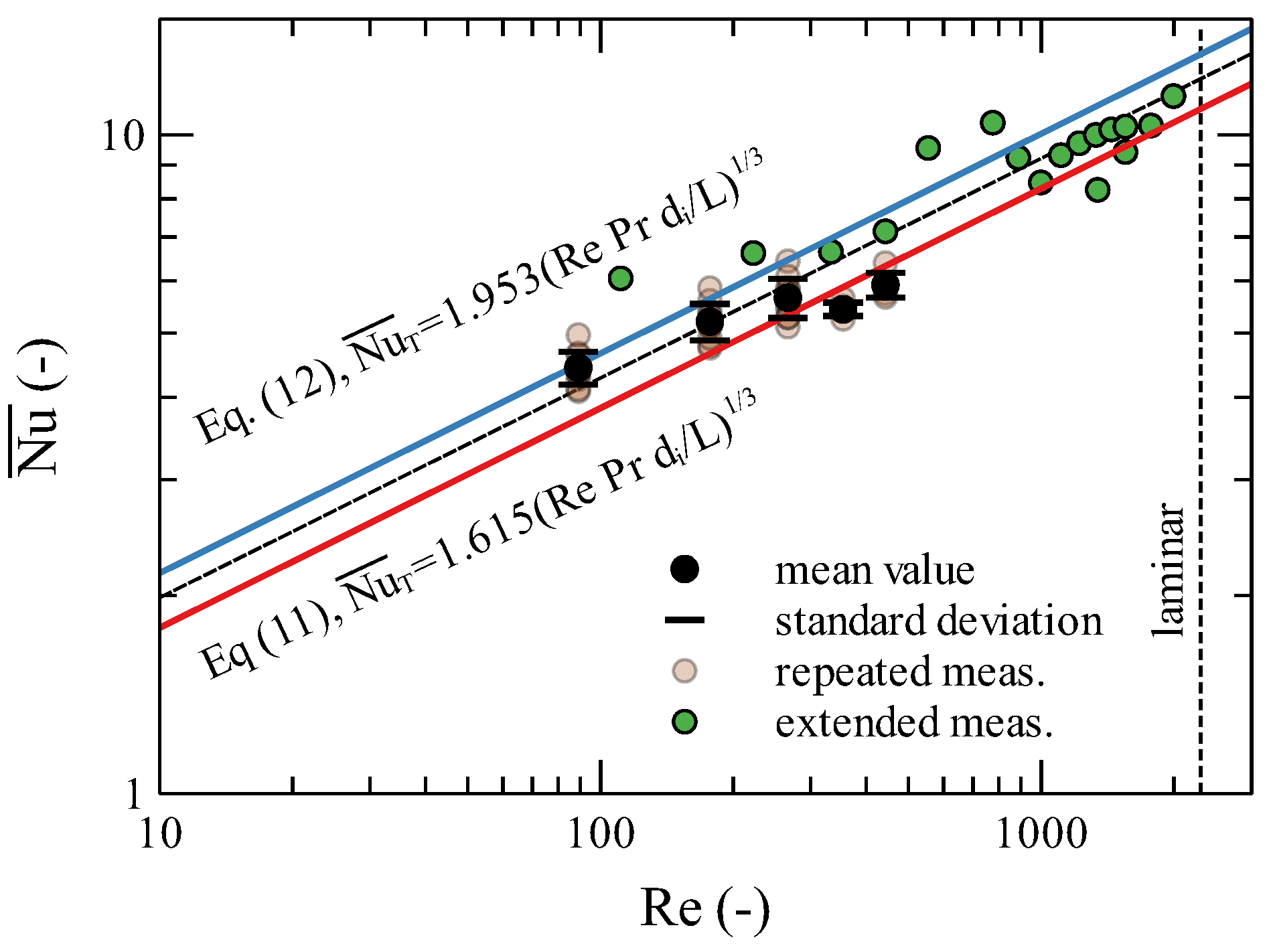
When comparing the average values of Nusselt numbers $\overline{\mathrm{Nu}}$ depending on the Reynolds number, we can judge that the experimental method measures relatively good values compared to Equations (11) and (12); see Figure 12.

From the comparison, we can see that the measured values correspond very well to the theoretical assumptions both in the repeated area and in the extended area of measurement. From all the measured values, we can evaluate the regression in the same functional dependence as Equations (11) and (12) and obtain

$${\overline{\mathrm{Nu}}}_{\sin }=1.843{\left[\mathrm{Re}\mathrm{Pr}(d_i/L)\right]}^{1/3}[R^2=0.9743]$$

(21)

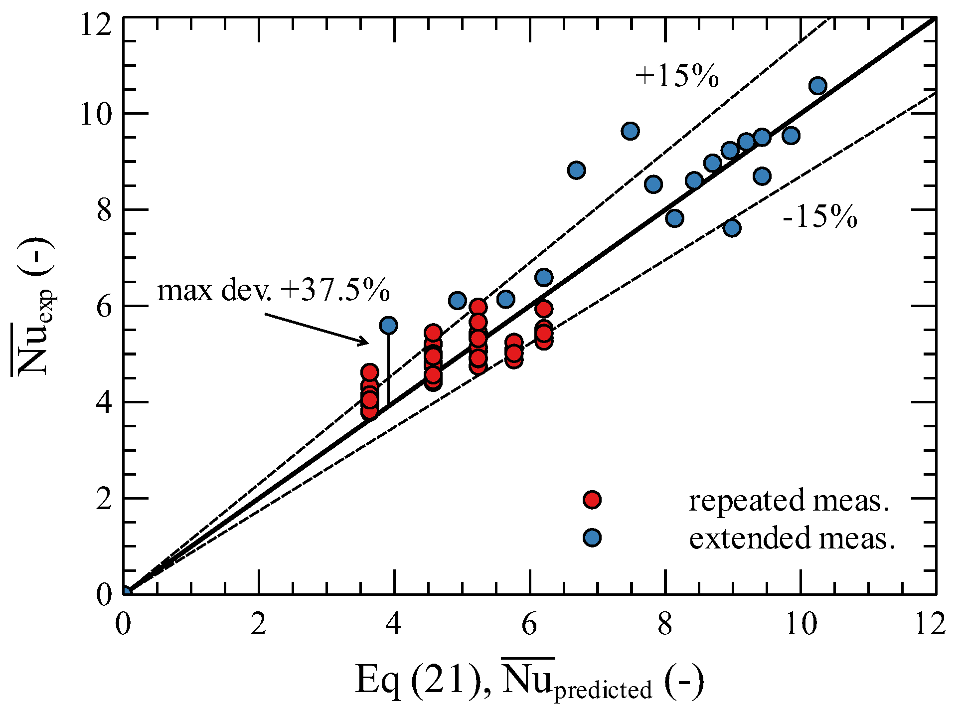
The measured values compared to the established correlation for ${\overline{\mathrm{Nu}}}_{\sin }$ (see Equation (21)) can be seen in Figure 13. The maximum deviation of one point is 37.5%, the average deviation of all points is below 15%. The deviation of the data corresponds to the estimated accuracy of the method.

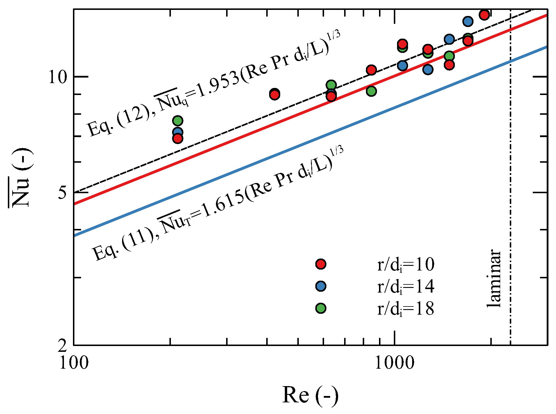
When measuring bent pipes, the procedure was such that the measured data of the new experiments were compared with the data and correlations for straight horizontal pipes. The area-averaged values of Nusselt numbers depending on the Reynolds number can be seen in Figure 14.

It can be seen that the average values of the Nusselt number are higher than in the case of a straight horizontal pipe. However, practically no difference or dependence on the bending radius of the tube can be seen. Therefore, only one regression is performed for all measured values of the pipe bend radius and the result is:

$${\overline{\mathrm{Nu}}}_{\sin ,90}=2.201{\left[\mathrm{Re}\mathrm{Pr}(d_i/L)\right]}^{1/3}[R^2=0.8750]$$

(22)

If a two-parameter regression is performed (the second parameter would be the exponent) on all measured data with 90 degree band, the resulting correlation would be:

$${\overline{\mathrm{Nu}}}_{\sin ,90}=2.895{\left[\mathrm{Re}\mathrm{Pr}(d_i/L)\right]}^{0.293}[R^2=0.8571]$$

(23)

we see that there is a slight deviation of 1/3 of the exponent value compared to the theoretical estimate. The deviation is not fundamentally significant, so it is possible to use the correlation with the original exponent.

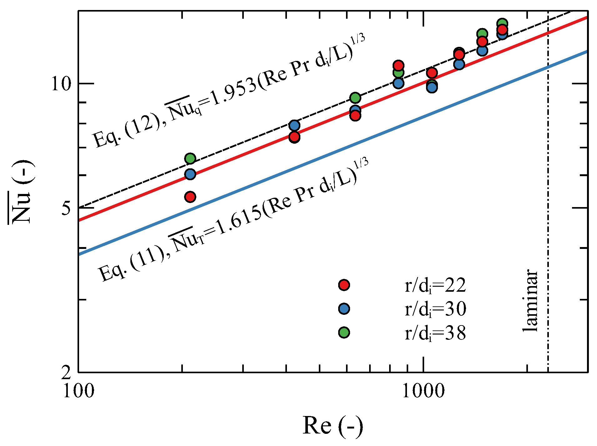
We can perform a similar procedure for measured data with a pipe bent by 180 degrees. The dependence of the average Nusselt numbers on the Reynolds number is shown in Figure 15.

We can see that the measured Nusselt numbers are again higher than for a straight horizontal pipe and even a little higher than for a 90 degree bend in the pipe. However, again, we cannot see any dependence on the bend radius. We obtain a one-parameter regression with a fixed exponent:

$${\overline{\mathrm{Nu}}}_{\sin ,180}=2.153{\left[\mathrm{Re}\mathrm{Pr}(d_i/L)\right]}^{1/3}[R^2=0.8571]$$

(24)

and if a two-parameter regression is performed:

$${\overline{\mathrm{Nu}}}_{\sin ,180}=1.674{\left[\mathrm{Re}\mathrm{Pr}(d_i/L)\right]}^{0.366}[R^2=0.8333]$$

(25)

Again, we see that the exponent deviates very slightly from the theoretical value of 1/3, but again it is not a fundamental deviation, so we will use one-parameter regression.

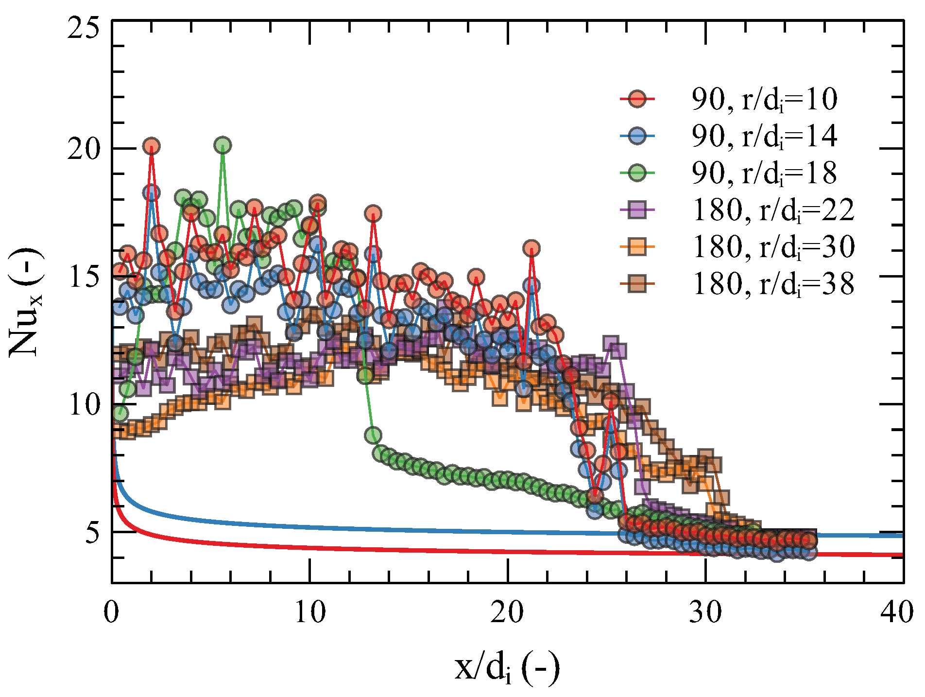
The local values of Nusselt numbers from the entrance to the measuring section are also compared and the results can be seen in Figure 16. From Figure 16, we can see that the bends fundamentally distort the shape of the local values of the Nusselt numbers. Both bending geometries along the heat exchange surface gradually settle back to the values predicted for straight horizontal pipes.

6. Dicussion

The first task was a numerical study of laminar flow with a time-varying Cauchy boundary condition. For that task, the analytical solution was not available and therefore the numerical calculation of this problem was chosen. It follows from the solution that most probably the oscillating heat flux partially deforms the shape and that the resulting values of the Nusselt number lie between the two boundary conditions of the first ($T=\mathrm{const}.$) and second ($q=\mathrm{const}.$) kind.

Experiments performed on a straight horizontal pipe confirmed these results. The measured data after repeated experiments and their averaging corresponded to this solution. However, it is not possible to decide on the deformation of the Nusselt number profile from the beginning of the measurement zone and it is necessary to choose a measuring method that is at least an order of magnitude more accurate and sensitive. At the beginning of the measurement zone, a partial deviation from the already known equations for determining the local Nusselt number can be seen; it is also an area where a large derivation of values occurs. Freund [24] wrote about such gradients indicating that the error of the method increases here and so this inaccuracy is most likely related to this phenomenon.

By comparing the regressions with a fixed value of the exponent at 1/3 of the theory, we can calculate the deviations from the behavior in a straight horizontal pipe. For a 90 degree pipe bend, this change is +16.5% and for a 180 degree bend the change is 16.8%.

The average values of the Nusselt numbers depending on the Reynolds number turn out to be reasonable both in the region of repeated measurements (Re = 100–700) and in extended region (Re = 100–2000). From this dependence, a correlation with the same functional prescription as for boundary conditions of the first and second kind was derived. Even in average values, this correlation lies in the region between the two functions. The deviations from the predicted correlation are significant, which can be expected for a dynamic method with intense heat transfer. The estimated inaccuracy of the method for this application is $\pm 10$ to $\pm 15\%$. The largest deviation from the prediction was 37.5%, but the vast majority of measured data has a deviation smaller than 15%.

In experiments with bent tubes, a disruption of the laminar flow is evident, which results in a change in the heat transfer coefficient. Local values show fundamental differences from straight horizontal pipes. Very similar behavior was observed in [34], where flow turbulizers were installed in a squared tube with turbulent flow.

The increase in the values of the heat transfer coefficient is due to the disturbance of the boundary layer that has formed at a sufficiently long settling length. This boundary layer represents the diffusive thermal resistance in direct relation to its thickness. Bending of the pipe or any other obstacle (e.g., turbulizer) distorts the boundary layer and reduces its thickness, thereby increasing heat transfer.

Other sources have reported on the dependence of the heat transfer coefficient on the radius of rounding and the Reynolds number, with numerical simulations registering similar increases; see Patro et al. [9]. In our experiments, the dependence on the Reynolds number was clearly verified, but the dependence on the turning radius was not evident. This is most likely caused by insufficient sensitivity of the measuring method.

Changing the values of the heat transfer coefficient and therefore the Nusselt number, does not change the nature of the flow inside the pipe in its fold. If the character of the flow were to change in a fundamental way (e.g., a vortex in the flow were to break off), this would be evident in the change in the exponent of the Reynolds number. A typical value of the exponent for a fully developed internal flow in pipe is 4/5. This change was not observed and the experimental results are consistent with the exponents predicted by the analytical solution (exponent of the Reynolds number 1/3).

The dependence of the Prandtl number for correlations tends to be the same for laminar flows (and in some cases also for turbulent flows), if they are of the Newtonian type. In the literature, correlations can be found for a wide range of Prandtl numbers; e.g., Taler [35] presented a modified Gnielinski correlation for a large number of fluids and for a range of Prandtl numbers 0.1–1000.

7. Conclusions

In this work, numerical and experimental measurements of laminar water flow in a pipe with a non-standard boundary condition, i.e., oscillatory heat flux at the pipe wall, have been carried out. The numerical study showed that the solution of such a problem is found in the interval between two standard boundary conditions, namely the first kind T = const. and the second kind q = const. However, we propose a much broader and more thorough numerical analysis to draw deeper conclusions concerning this problem.

The experimental results confirm the numerical ones, the measured values on the plane tube show the same tendency of the average values of the Nusselt number on the Reynolds number and the same is the case for the local values from the beginning of the measuring zone. The deviations from the established correlations are approximately the same as the inaccuracy of the dynamic measurement method used, the consistency of the local data is at a very good level and the repeatability of the experiment is also good.

In the experiments with bent tubes, we observed a significant change in the value of the heat transfer coefficient, but the changes as a function of the bending radius are relatively small and below the resolution of the method. We therefore decided to run a regression on all the data measured for a given bend (90 or 180 degrees) and the $R^2$ values show that there is no fundamental problem. In order to determine the dependence of the change in the heat transfer coefficient on the bending radius of the pipe, it is necessary to use other measurement methods with higher resolution.

From the measured data we can see a fundamental distortion in the shape of the local heat transfer coefficient values from the beginning of the measurement zone. The fundamental distortion of this shape can be seen at the fluid inlet of the measuring section, but after a certain distance we can observe that this distortion reduces its impact on the results and returns back to the values predicted by the correlations for the plane tube.

All measured results have been converted into correlation form and are presented in the

Table 2. Determined correlations for individual geometries and their limitations.

Channel Geometry	Nu Number Correlation	${\mathit{R}}^2$ Value	Limitations
straight	$1.843{\left[\mathrm{Re}\mathrm{Pr}(d_i/L)\right]}^{1/3}$	0.9743	Pr = 7, Re = 50–2300
bend 90	$2.201{\left[\mathrm{Re}\mathrm{Pr}(d_i/L)\right]}^{1/3}$	0.8571	Pr = 7, Re = 50–2300, $r/d_i$ = 10–18
bend 90	$2.895{\left[\mathrm{Re}\mathrm{Pr}(d_i/L)\right]}^{0.293}$	0.8571	Pr = 7, Re = 50–2300, $r/d_i$ = 10–18
bend 180	$2.153{\left[\mathrm{Re}\mathrm{Pr}(d_i/L)\right]}^{1/3}$	0.8571	Pr = 7, Re = 50–2300, $r/d_i$ = 22–38
bend 180	$1.674{\left[\mathrm{Re}\mathrm{Pr}(d_i/L)\right]}^{0.366}$	0.8333	Pr = 7, Re = 50–2300, $r/d_i$ = 22–38

with $R^2$ values and usage limits:

There are several findings from the study that will be part of further investigation:

• The numerical simulation shows that it is possible to use the temperature oscillation method to measure heat transfer coefficient values even in laminar flow with sufficient accuracy.
• The experimental results confirm the results from the numerical simulation. The Nusselt number correlations for the studied problem are very similar to those analytically derived for standard boundary conditions. The shape of the local values of the heat transfer coefficient at the entrance of the measuring section looks very similar.
• The resulting correlation of the Nusselt number for the straight pipe and for the oscillatory heat flux as boundary condition reproduces the dependencies of the standard boundary conditions, the correlation constant being between the values of the constants of the standard boundary conditions.
• Any bending of the pipe results in a distortion of the boundary layer and a change in its thickness, which results in a fundamental change in the heat transfer coefficient. This change is not permanent and the local heat transfer values along the flow axis return to the original values.