Optimal Energy Management System of Isolated Multi-Microgrids with Local Energy Transactive Market with Indigenous PV-, Wind-, and Biomass-Based Resources

Abstract

The availability of sustainable, efficient electricity access is critical for rural communities as it can facilitate economic development and improve the quality of life for residents. Isolated microgrids can provide a solution for rural electrification, as they can generate electricity from local renewable energy sources and can operate independently from the central grid. Residential load scheduling is also an important aspect of energy management in isolated microgrids. However, effective management of the microgrid’s energy resources and load scheduling is essential for ensuring the reliability and cost-effectiveness of the system. To cope with the stochastic nature of RERs, the idea of an optimal energy management system (EMS) with a local energy transactive market (LETM) in an isolated multi-microgrid system is proposed in this work. Nature-inspired algorithms such as JAYA (Sanskrit word meaning victory) and teaching–learning based optimization algorithm (TLBO) can get stuck in local optima, thus reducing the effectiveness of EMS. For this purpose, a modified hybrid version of the JAYA and TLBO algorithm, namely, the modified JAYA learning-based optimization (MJLBO), is proposed in this work. The prosumers can sell their surplus power or buy power to meet their load demand from LETM enabling a higher load serving as compared to a single isolated microgrid with multi-objectives, resulting in a reduced electricity bill, increased revenue, peak-average ratio, and user discomfort. The proposed system is evaluated against three other algorithms TLBO, JAYA, and JAYA learning-based optimization (JLBO). The result of this work shows that MJLBO outperforms other algorithms in achieving the best numerical value for all objectives. The simulation results validate that MJLBO achieves a peak-to-average ratio (PAR) reduction of 65.38% while there is a PAR reduction of 51.4%, 52.53%, and 51.2% for TLBO, JLBO, and JAYA as compared to the unscheduled load.

1. Introduction

Access to sustainable, reliable, and affordable energy services is vital for developing and rural communities’ viable growth and achieving universal, sustainable energy access by 2030. The desire for electricity and energy is not an extravagance but a necessity now in this global world [1]. Although the share of people with access to electricity grew over the past decade, more than 759 million people still lack this basic need to achieve United Nation’s Sustainable Development Goal #7 aiming at access to affordable electricity [2]. The residential sector is the largest electricity consumer, which accounts for 39% of total electricity consumption in the USA in 2021 [3]. Much electricity in homes and buildings is lost because of the absence of an energy management system (EMS), either due to the negligence of the owners or due to the cost associated with this technology. Innovative automatic electricity management solutions can help reduce overall energy costs, flatten the load curve, and shift the peak loads to off-peak hours while maintaining a tolerable discomfort level [4].

In the current era of sustainable energy, it has been a great challenge for the government to provide electricity due to technical and economic infeasibility, and alternative solutions must be sought. The excessive cost associated with the transmission infrastructure required to provide access to electricity for off-grid communities far exceeds the revenue generated by selling electricity [5]. The inclusion of distributed energy resources (DER) and the inclination toward renewable energy resources (RER) lead to a smaller local distribution system known as microgrids (MG). Microgrids have several advantages, such as increases in the system’s reliability and flexibility of the grid for future expansion [6]. It can be connected in either a grid-connected topology or an isolated mode. A distinct characteristic of MGs is to have well-defined boundaries with adjustable loads and multiple generation options to account for the uncertainty of the energy output from renewable energy resources (RER), i.e., photovoltaic (PV) and wind energy [5,6,7].

The benefit of local generation at the consumer’s premises leads to reduced energy bills, reduced cost of distribution as no transmission infrastructure is needed, and less stress on the utility grid if it is a grid-connected configuration as it can cover the load demand of both the consumer and the utility needs. The decentralized isolated microgrid (IMG) topology has several benefits compared to its contemporary, the traditional centralized power grid, such as more reliability, flexibility, self-sufficiency, being self-automatic, and intelligence [8]. Other intelligent technologies further assist MG in incorporating control management, such as demand-side management (DSM) for rescheduling the load when the generation is insufficient. Electricity generation is not always available to meet the load demand, so it must include an energy storage system (ESS) to meet the extra demand that the generation sources cannot provide, thus reducing the cost of electricity and consumer discomfort [8,9].

The clustered arrangement of MGs, often regarded as multi-microgrids (MMG), can be more efficient and comparatively have better techno-economic benefits with more adaptability and resilience than a single MG. Some focused research areas associated with MMG are frequency control, protection, and system stability. Several control strategies have been adopted to mitigate the impact of varying energy output from RER, such as DSM and demand response (DR). The authors of [10] used a similar approach for isolated microgrids, which used the frequency-based DR strategy for thermostatically controllable loads (TCLs) to provide primary frequency control. The hybrid TCL-based DR approach resulted in higher RER penetration with better frequency regulation. A novel combination of adaptive droop control (ADC) and model predictive control (MPC) is proposed by the authors of [11] for frequency regulation in IMG, along with a genetic algorithm for parameter tuning. An optimal and robust adaptive-droop-control-based approach is used for frequency and active power regulation after a disturbance in the system for IMMG [12].

Currently, the available literature focuses on the control strategies for isolated and grid-connected MMG, while some methods focus on the constraints-based and protection design for MMG configurations. The fault current in MG with high penetration of RER comes with the issue of slow inertial response to faults resulting in fault currents that far exceed the power electronic converter (PEC) ratings if not dealt with promptly. A state-of-the-art differential fault detection and fault phase identification method is proposed in [13] for IMG, which uses edge computing features at both nodes for fault detection rather than the differential current with high accuracy and swift response. In [14], a grounding and protection strategy is proposed to focus on maintaining a significant level of grounding coefficient (COG) and overvoltage ratio in case of phase fault but lacks a practical proof of concept. A novel EMS approach accounting for second-to-second power fluctuations in RER is proposed in [15]. The bulk dynamic simulations for frequency regulation reduced operation and computational cost while achieving a wider range of frequency regulation security levels. However, due to the linear nature of equations, the computation cost increases significantly with the system’s size. Authors in [16] proposed an optimal design of isolated microgrids based on mixed-integer linear programming (MILP) with multiple DER and with a constraint on energy security and the effective use of electrical and thermal energies. This paper aimed to design integrated microgrids with the optimal mix of RER, size, and placement of DER while concurrently reducing the operation cost and energy security risk. However, RERs were not included in the optimized dispatch model, thus limiting the effectiveness of this approach to the traditional DER.

Various methods have been proposed considering load management, cost optimization, and optimal storage sizing. In [17], an energy management system with a semi-local market mechanism based on an MPC strategy for a grid-connected MMG was proposed with a focus on the energy regulation and the economic effect of rescheduling MG components in a grid fault condition. In [18], a multilevel design approach for the optimal size of ESS for a single grid-connected MG based on an advanced grey wolf particle swarm optimizer (AGWPSO) was proposed with the objective of reduced load shedding, cost, and payback period. In [19], a multistage EMS for an MMG connected to the utility grid focuses on energy cost reduction with minimum load interruptions based on day-ahead and real-time energy trading. In the first stage, resources are scheduled to minimize the cost, while the energy trading algorithm optimizes ESS use in the second stage. The authors of [20] proposed a hierarchical electrical power market framework for interconnected intelligent buildings to reduce the peak-to-average ratio (PAR), user discomfort, and electricity cost in grid-connected configurations. The proposed model was compared with different case studies, including electrical vehicles (EV), and showed reduced PAR and price compared to the base case.

In addition to the above mention studies, some studies use a combination of energy trading and EMS for MMG. Most of these incorporate a semi-local power market where the prosumer has the choice of either selling extra electricity to the grid at a reduced price or by the effective use of ESS during peak hours to refrain from buying expensive electricity. The opportunity of trading electricity at cheaper unit rates with neighboring grids reduces the economic stress and encourages the deregulated power market mechanism in isolated multi-microgrid (IMMG). Much research work has been done using different heuristic and meta-heuristic techniques to optimize revenue and reduce the cost of electricity. A day-ahead predictive framework based on a cascaded MPC is proposed for peer-to-peer energy trading in [21]. Amr et al. [22] proposed mixed-integer nonlinear programming (MILNP) based on an optimized planning and sizing approach for a hybrid AC/DC configuration to reduce the levelized investment cost. A popular heuristic algorithm is the grey wolf optimization technique (GWO) which gives accurate results and fast convergence of a slow dynamic response [23]. Another commonly used algorithm for economic scheduling is particle swarm optimization (PSO) [24]. Although PSO gives a computational speed advantage, the inability to solve discrete optimization problems associated with it limits its application.

Improved optimization results are obtained using a hybrid algorithm inspired by nature, such as the hybrid Genetic Algorithm (GA)–Simulated Annealing (SA), which uses load scheduling and is optimized using GA. The parameter tuning is done through SA [25]; the modified grasshopper optimization algorithm (MGOA) is used for the economic dispatch objective function in [26]. For problems with a high number of input variables, modern artificial-intelligence-based methods are used for system stabilization with a high injection of RER. A novel salp swarm optimization algorithm (SSA) is used for a superior frequency response and power quality optimization during load switching. The dynamic behavior of the grid-tied system is improved with high DER penetration and compared with the grasshopper optimization algorithm (GOA) [27]. Charge scheduling of EV is proposed using an advanced metering infrastructure (AMI)-based artificial neural network (ANN) in [28]. Deep learning (DL) and deep reinforced learning (DRL) methods are used for optimal dispatch in [29]. An Internet of Things (IoT)-based deep learning method is proposed for a group of microgrids with EV and RER for reduced carbon emission and maximum revenue [30].

Although tremendous work has been done in the various aspects of IMG and MG, most research focuses on control and stability in the grid-connected MG mode and isolated mode. The optimization of different objectives with multiple algorithms has been published in current literature. Metaheuristic algorithms such as PSO, GWO, and GA require algorithm-specific parameters and continual performance tuning of parameters. A minute change in any parameter results in a significant difference in the algorithm’s performance. These algorithms suffer from premature convergence and can be stuck in the optimal local solution. Particle swarm optimization (PSO) is known for its robustness and global search capability, but it suffers from parameter tuning. The PSO algorithm has some parameters that need to be set before running the optimization process such as number of particles, inertia weight, cognitive and social coefficients, etc. These parameters have a significant impact on the performance of the algorithm. If the parameters are not set correctly, the algorithm may not converge to the global optimal solution or may converge too slowly. The algorithms such as the aquila optimizer algorithm and whale optimizer algorithm (WOA) both lack the capability of constraint handling and multi-objective optimization and attempted to address the constraint handling issue by incorporating different constraint handling techniques such as the penalty function method, feasible region method, and repair method [31,32]. The merits and demerits of algorithms discussed in the literature are summarized in

Table 1. Literature summary.

Ref	Method	Technologies						System		Advantages	Disadvantage
		PV	Wind	Biomass	Hydro	Diesel	ESS	Islanded	Grid Connected
[9]	KBES	-	√	-	-	√	√	√	-	Fast decision speed and flexible implementation	Complexity, limited knowledge.
[11]	ADC	√	√	-	-	√	√	√	-	Good stability, fast response, simple to implement	Requires advanced genetic algorithm for parameters tuning.
[17]	MPC	√	√	-	-	√	√	√	-	Cost-effective and enhanced energy saving	Complex to design and implement, high computational cost.
[19]	DA, RT	√	√	-	-	-	√	-	√	More flexible, fast response to uncertainties	Complex to implement simultaneously, increase computation.
[20]	JAYA	√	√	-	-	-	√	√	-	Does not require complex parameter tuning, adaptability	can get stuck in local optima and sometime does not converge.
[21]	Cascaded MPC	√	√	-	-	-	√	-	√	Improved performance as compared to MPC	Requires additional tools for parameters tuning.
[22]	MILP	√	√	-	-	√	√	√	-	Global optimization and flexible for variety of solvers	Complexity, Long time for solution and limited to low dimensional problems.
[23]	GWO	√	√	-	-	√	-	-	√	Constraint handling, high convergence rate	High computational intensity, significant parameters tuning.
[24]	PSO	√		-	-	√	√	√	-	Have moderate convergence speed, can be used for complex	Difficult to optimal tune parameters, can trap easily in local optima.
[25]	GA-SA	√	√	-	√	√	-	-	√	Multi-objective and multi-constraint handling	Slow convergence, require additional algorithm for parameters tuning.
[26]	MGOA	√	√	-	-	√		-	√	Improved exploration and fast convergence	Sensitive to method of parameters initialization.
[28]	ANN	-	-	-	-	√	√	-	√	Can manage large number of data and input variables. Trustable predictions	Large training data set and high computational cost.
[30]	DL	√	√	-	√	√	√	√	-	Real time scheduling, improved uncertainty predictions	Expensive computation, extensive training for reinforced learning is required.

.

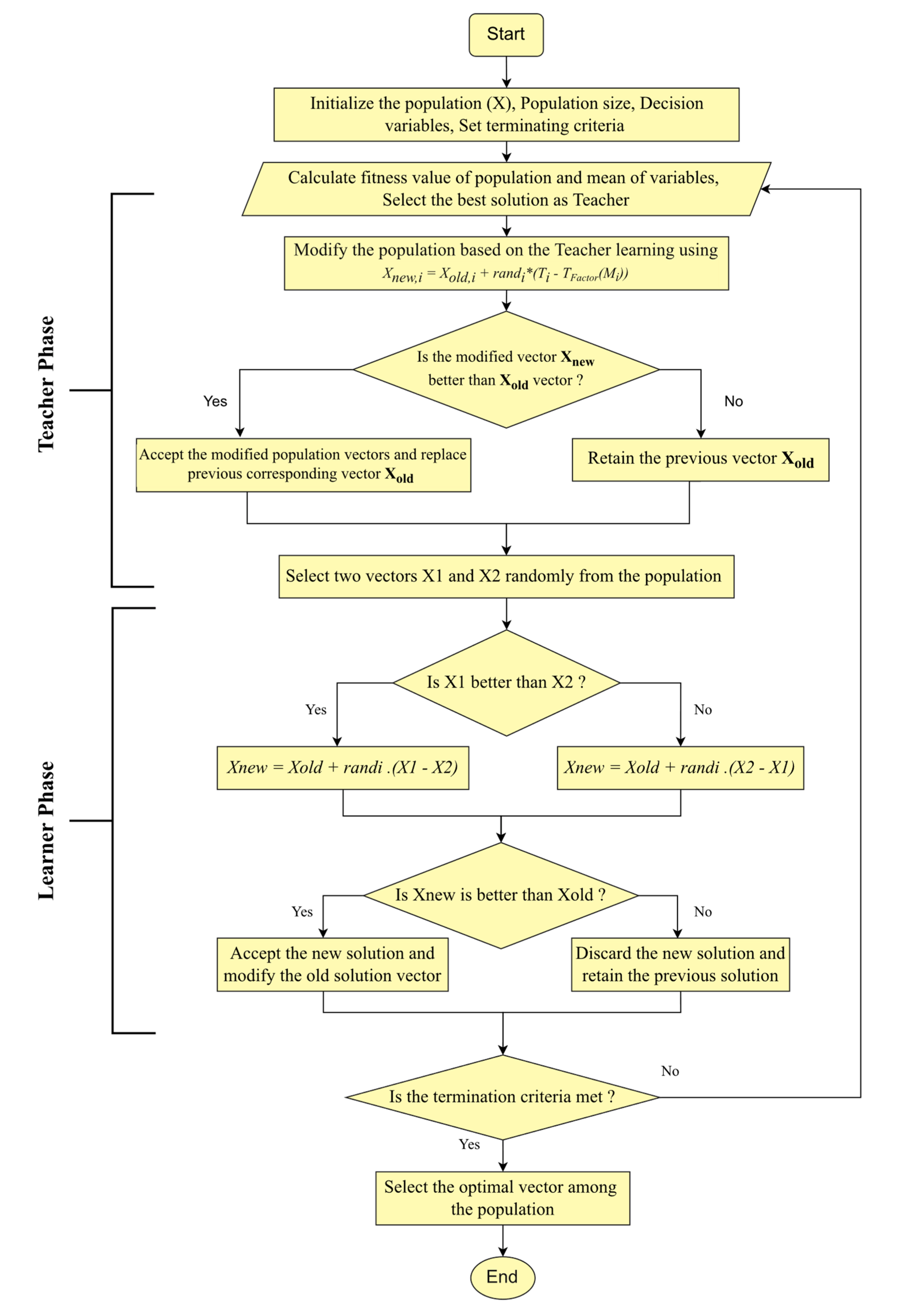
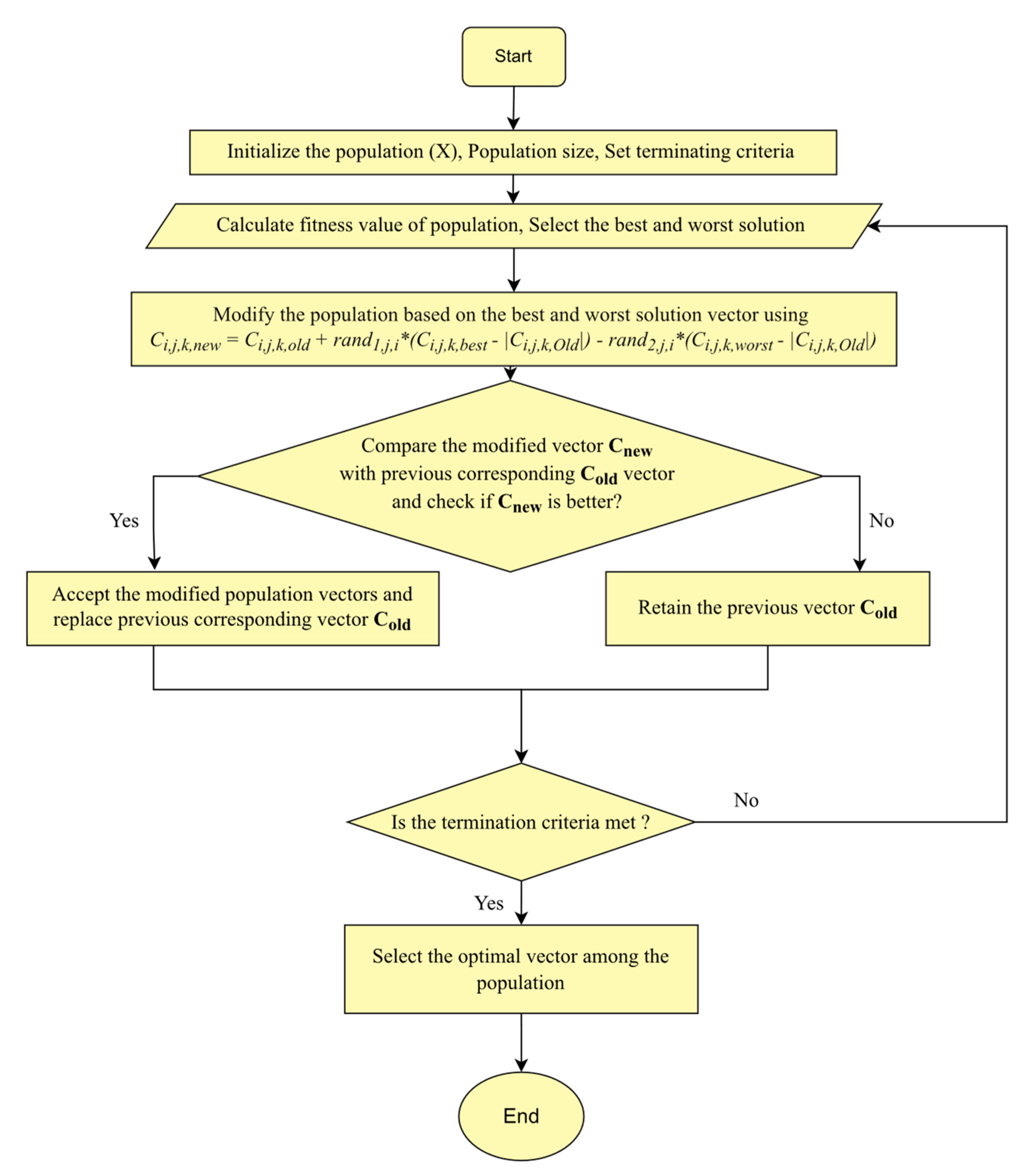
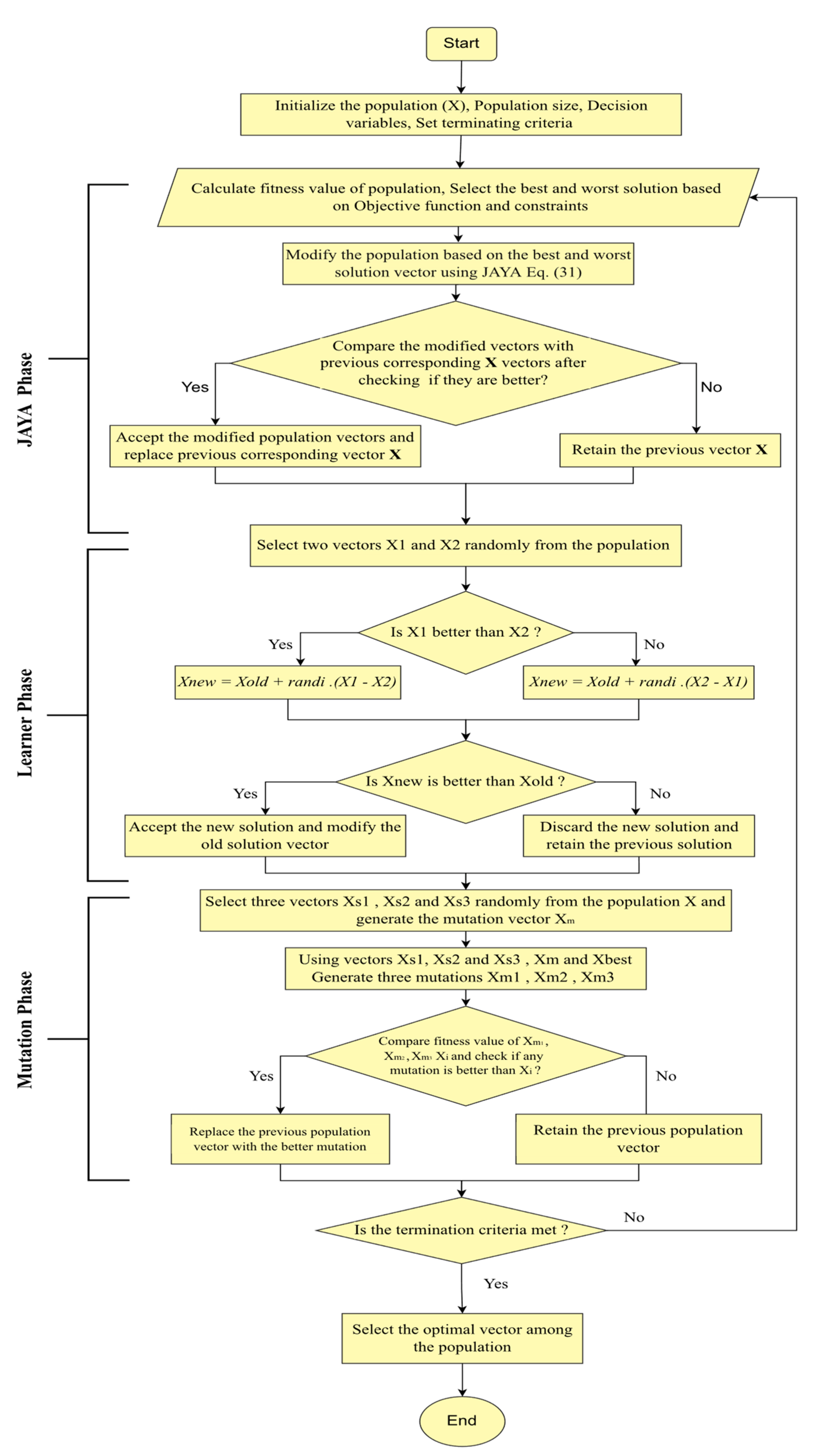
Therefore, algorithms such as JAYA (Sanskrit word for triumph) [33] and teaching–learning-based algorithms (TLBO) [34] have been proposed in recent literature, which do not require parameter tuning. Their input parameters are just the population size and number of generations, making them less complex to implement. Hybrid techniques of these algorithms, such as the JAYA teaching–learning-based algorithm (JLBO), have also been used for the optimal sizing of hybrid RER in a single microgrid [35]. During the learner phase, the JLBO algorithm can get stuck in local minima due to the bad learning of students.

However, to the best of the author’s knowledge, limited literature is available regarding IMMG, and the energy management of IMMG is not contemplated in the literature. Hence, a novel modified JAYA teaching–learning algorithm (MJLBO) is proposed in this work. One of the key advantages of the modified JLBO algorithm (MJLBO) algorithm is its ability to explore the search space effectively and quickly, while avoiding getting stuck in local optima. This is achieved by combining the global search capability of JAYA and the local search capability of TLBO. Additionally, the JAYA-TLBO algorithm can also handle constraints effectively, which is important in the energy management system scenario. The algorithm can balance the trade-off between the objective function and the constraints by adjusting the parameters of the TLBO algorithm and can handle multiple objectives in a multi-objective optimization problem, which is a common feature in the energy management system. This is a novel research topic, as it has not been widely studied yet, and it addresses the specific challenges of providing electricity to rural areas through multiple isolated microgrids.

The following are the contributions of this work:

• An optimal time of use (TOU)-based deregulated power market for IMMG, where each MG can freely participate in the local energy transactive market (LETM) and trade energy with the neighboring grids without including the utility grid.
• An efficient modified JLBO algorithm (MJLBO) is proposed for an optimal microgrid EMS (MEMS) for an objective function comprising multiple objective scheduling problems, such as minimizing the electricity cost, reducing the peak-to-average Ratio (PAR), and maximizing the use of ESS and RES while considering user preference.
• Multi-objective constraints modeling with constraints handling capability for the IMMG energy management system.
• We also considered biomass energy resources and modern loads such as electrical vehicles (EVs) in interconnected MEMS.
• Evaluation and validation of the proposed framework are done against multiple case scenarios.

The remainder of this paper is organized as follows: Section 2 presents the proposed system architecture and components’ modeling. Section 3 presents the objective function along with the constraints of the system components. In Section 4, the proposed algorithm and bench test algorithms are discussed. Section 5 presents the simulation results and discussion. Finally, the conclusions are presented in Section 6.

2. Proposed System Architecture and Component Modeling

2.1. System Setup

The proposed IMMG setup consists of three smart MGs isolated from the main utility grid, as shown in Figure 1. The proposed system consists of the single AC bus architecture with the complete hybrid renewable system (HRES) to accommodate 100% RER where each MG is dominated by solar PV arrays, wind turbine (WT), and biomass (BM) energy sources, respectively. Due to the intermittent nature of renewable energy sources, the system will be unstable as the input power will not be enough to cater to the load demand. Hence, each MG consists of a battery energy storage system (BESS) comprising battery banks to avoid the resultant power mismatch and acts as an energy buffer. Each MG comprises six homes, further subcategorized into three economy classes, i.e., rich, medium, and small, as shown in Figure 2.

All load appliances in each home are equipped with smart energy meters and are connected to the central control unit, which schedules the devices in the appropriate hour windows while respecting the user-provided time horizon. The load appliance’s power rating, scheduled starting and ending time slot, and length of operation for each load are presented in

Table 2. Load appliance parameters.

Subclass	List of Appliances	Power Rating (kW)	Starting Slot	Finishing Slot	OTS
	Washing machine	0.5	47	60	3
	Refrigerator	0.225	1	120	119
	Electrical iron	1.2	35	42	2
	Table fan	0.025	50	100	25
	Ceiling fan	0.1	1	120	90
Low, Medium, Rich	Coffee grinder	0.1	42	45	1
	Water pump	1	1	120	3
	Vacuum cleaner	1	46	55	3
	Lights	0.15	1	120	70
	Laptop	0.25	1	120	20
	TV	0.1	40	120	25
	Dryer machine	3	80	115	3
	Water heater	2	80	100	3
Medium, Rich	Air conditioner 1	1.2	60	80	20
	Air conditioner 2	1.2	100	120	10
	Microwave oven 1	1.5	38	44	2
	Microwave oven 2	1.5	88	102	4
	Electrical stove 1	1.5	40	45	1
Rich	Electrical stove 2	1.5	85	100	2

^{1, 2} Represents the times these loads are scheduled more than once.

. Since some appliances such as coffee grinders do not need to be operated for an hour, each hour is divided into five 12 min time slots; appliances must not start outside the starting and ending slot window. Each appliance can operate more than once, but the user needs to define its different time horizons. Other system components included in the proposed setup are the battery energy management system (BEMS), the home energy management system (HEMS), and the MG energy management system (MEMS).

The proposed approach discusses three power modes: surplus, deficit, and power balance. Each MG participates in energy trading in the proposed deregulated market mechanism so that each MG community’s overall electricity cost and discomfort level are minimal. In surplus mode during daylight, when PV dominates in MG, BESS stores surplus RE generation during peak RER hours, and the remaining power is traded with the other MGs at separate tariffs. Similarly, surplus energy is stored in their BESS when the WT system outputs more power than its respective MG load demand. During the deficit period, MG first utilizes its BESS stored power. The remaining energy is taken from the other two MG at their respective time-of-use (TOU) tariffs. The third biomass-dominated MG acts as a slack bus that outputs constant power throughout the day at its tariff. Later, the devices will be powered by BESS at high electric prices. Thus, each MG can participate in the energy transactive market and sell the surplus electricity produced via RER or BESS to the neighboring MG.

2.2. Modeling of Components

The microgrid architecture under study consists of 100% RER and battery system as energy storage. This section presents the detailed formulation modeling of all resources including RES, BESS, and EV.

2.2.1. Modeling of EV

Many factors affect the exact modeling of EV but, for our study, we focused on electrical prospects, specifically the battery SOC, duration of the plugin, and correlation with the driving distance. We considered the following discrete-time modeling for EV batteries [36,37]:

$$SO{C}_{EVB,i+1 }=\left\{\begin{array}{l}SO{C}_{EVB}^{min} ,\hspace{1em}if \left(SO{C}_{EVB,i}-\frac{d}{Ef{f}_{EVB}\times Q_{EVB}} \right) \le SO{C}_{EVB}^{min}\\ SO{C}_{EVB,i}-\frac{d}{Ef{f}_{EVB}\times Q_{EVB}}\hspace{1em},\hspace{1em} Otherwise\end{array}\right.$$

(1)

where SOC_EVB,i and ‘d’ are the given parameters for the previous state of charge of the battery and distance traveled. Here, the state of charge is lower-bounded to avoid the over-discharging and depletion of the battery. The charging process of EV batteries is governed by Equation (2):

$$SO{C}_{EVB,i+1 }=\left\{SO{C}_{EVB,i}+\frac{P_{EVB,i}\times \Delta t}{Q_{EVB}}\right.\times 100\%$$

(2)

where:

• Eff_EVB—Net drive electric efficiency (km/kWh)
• SOC_EVB,i—State of charge during the plug-out time (%)
• SOC_EVB,i+1—State of charge during the plug-in time (%)
• Q_EVB —EV battery capacity (kWh)
• P_EVB,i—Charging power at any given time (kW)
• $\Delta t$—Duration of each time slot (h)
• $SO{C}_{EVB}^{min}$—Minimum SOC of EV battery (%)

2.2.2. Modeling of BESS

Due to the stochastic nature of the renewable energy sources being employed, an energy buffer is essential for smooth microgrid operation. The purpose of BESS is to act as an energy buffer that can absorb extra energy and can provide stored energy back when needed in the microgrid. This benefits in reducing the peak load demands, reducing the load shedding, and maintaining power balance within the microgrid. Equation (3) governs the SoC of BESS at any ith time interval [38].

$$\left\{\begin{array}{l}Charging:\hspace{1em}SO{C}_{B, i} =\left[SO{C}_{B,i-1}+\left(P_{Bch,i}\times {\eta }_{B,ch} \right)\right]\times \frac{\Delta t}{Q_B}\\ Discharging: SO{C}_{B, i} =\left[SO{C}_{B,i-1}-\frac{P_{Bdis,i}}{{\eta }_{B,dis}}\right]\times \frac{\Delta t }{Q_B}\end{array}\right.$$

(3)

where SOC_B,i is the battery SOC at the ith interval, $\Delta t$ is the time interval of each slot, and $P_{Bch,i}$ and $P_{Bdis,i}$ are the charging and discharging power, respectively. ${\eta }_{B,ch}$ and ${\eta }_{B,dis}$ are the charging and discharging efficiency of battery, and $Q_B$ is the capacity of the battery. For this study, both efficiency values are considered 100% as an assumption of no losses in the process of charging and discharging. The battery can only be in a charging or discharging state in any given time slot.

2.2.3. Modeling of PV

The output power of the PV module is dependent on multiple factors such as the system power rating, solar irradiance, ambient temperature, and cell temperature. The relation between the PV array output power and the aforementioned factors can be described as [35,39]:

$$P_i^{PV}=P_{rated}^{PV}.\frac{S_i}{I_S} \left[1-{\eta }_T\left(T_c-{25}^{°}\right)\right]$$

(4)

It is noteworthy that cell temperature affects the panel efficiency and hence the output power. Therefore, the temperature effect on the PV panel power is considered where T_c is the cell temperature and dependent on ambient temperature (T_amb).

$$T_C=T_{amb}+\left(\frac{NOCT-{20}^{°} }{0.8\left(kW{m}^{-2}\right)} \right).S_i$$

(5)

Here, NOCT is the nominal operating cell temperature defined by manufacturer, and is defined at the conditions when ambient temperature is 20 °C and solar irradiance is 0.8 kWm⁻² with a wind speed of 1 ms⁻². ${\eta }_T$ is the temperature coefficient of the solar cell, S_i is the solar insolation (kWm⁻²) at ith interval, I_s is the standard solar irradiance with a value of 1 kWm⁻², and $P_{rated}^{PV}$ is the manufacturer-provided rated PV power. Due to the unavailability of on-ground data, a generic PV generation profile is taken for this study.

2.2.4. Modeling of WT

The working principal of WT is the law of conservation of energy. The kinetic energy of the air impacting the WT blades is converted into mechanical energy and to electrical energy through the wind turbine generator. The output power of the incoming wind is dependent on the kinetic energy of the wind, specifically the cube of the wind speed as given by Equation (6).

$$P_{Wind}=\frac{1}{2}\rho {\nu }^3$$

(6)

However, the extractable power from this potential is dependent on the design of the wind turbine structure and it cannot exceed the coefficient of power $(c_p=59.3\%)$ at STC conditions. Thus, the maximum power of the ideal WT is given by Equation (7):

$$P_{Wind}=\frac{1}{2}\rho {\nu }^3{c}_p$$

(7)

where $\rho$ is the standard air density valued at $1.226$ kg/m³ at a temperature of 15 °C and air pressure at sea level. Since the instantaneous air speed does not remain the same all the time, the electrical power from WT can be modeled as a piecewise function of wind velocity. A generic mathematical relation of power to instant speed can be described as [40]:

$$P_i^{WT}=\left\{\begin{array}{ll}0& if {\nu }_t < {\nu }_{cutin} or {\nu }_t> {\nu }_{cutout}\\ \left({\alpha }_1+{\alpha }_2.{\nu }_t+{\alpha }_3.v_t^2\right)\times P_{rated}^{WT}& if {\nu }_t>{\nu }_{cutin} and {\nu }_t<{\nu }_{rated}\\ P_{rated}^{WT}& if {\nu }_t>{\nu }_{rated} and {\nu }_t<{\nu }_{cutout}\end{array}\right.$$

(8)

where $P_{rated}^{WT}$ is the rated power of WT provided by the manufacturer; and α₁, α₂, α₃ are the coefficient for the wind turbine model. ${\nu }_t$ is wind velocity at any time instant. ${\nu }_{rated}$ is the rated velocity at which WT output the rated power, ${\nu }_{cutin}$ and ${\nu }_{cutout}$ are the cut-in and cut-out velocities, respectively. A generic generation profile of a 20 kW solar system and 15 kW wind turbine is shown in Figure 3.

2.2.5. Modeling of Biomass Generation System

Biomass is residue and waste from living things including wood dust, cattle dung, human waste, bagasse, and agriculture compost. The decomposition process disintegrates this waste material into gases such as carbon dioxide (CO2) and methane (CH4) without oxygen (O2). Biomass generation works on the principle that this biogas acts as combusting fuel, and the thermal energy is converted to mechanical energy through internal combustion eventually converting into electrical energy through a turbine. The relation between biofuel and output power is described in Equation (9) [41]:

$$P^{BM}=\frac{F_{cons}}{\dot{m}\times \Delta T}$$

(9)

where $P^{BM}$ is the output power of biomass generation, F_cons is the yearly fuel consumption (tons/year), $\dot{m}$ is the fuel consumption rate (kg/kWh), and $\Delta T$ is the annual operating duration in hours. The fuel consumption rate depends on multiple factors such as the low calorific value of the fuel used for combustion and the generator’s efficiency. In this study, the upfront cost of the biomass raw material is negligible and hence assumed to be 0 ($/kW) since it is locally available, but the operation and maintenance cost of the plant is considered.

2.2.6. Modeling of Operating Schedule of Appliances

Initially, each hour is split into five equal time slots and takes 12 min, resulting in 120 time slots in a day. The time slot is made small because some loads do not need to operate for one complete hour to complete their work such as coffee grinder. Therefore, the resolution time slot of 12 min was chosen as the smallest operation time for any appliance in the proposed study. Moreover, each house length of time (LOT) for each appliance can be set to an integer multiple of 12. Hence, the unit of LOT is number slots. We assumed that to round off any operation time of an appliance closer to the integer multiple of 12 equals to the integer multiple; for example, if air conditioner has an operation time of 63 min which is close to 60 min (LOT of 4), the LOT for air conditioner is set to 4. However, this approach would produce some mistakes in the results, but these are small enough to be overlooked and are for only a few minutes. The total power consumption in the combined MMG system is given as follows:

$$P_{A }={\displaystyle \sum }_{a=1}^A{P}_a$$

(10)

$$P_{L, total }={\displaystyle \sum }_{N=1}^{N_G}{\displaystyle \sum }_{i=1}^T{P}_{A,i}^N\times S_a^i$$

(11)

where $P_{a,i}$ represents the power consumption in kWh for appliance ‘a’ for the ith time slot in microgrid ‘N’. $S_a^i$ is the ON/OFF state of that appliance at the ith time slot. The number of appliances is denoted by a = {1, 2, ……$A$}, the number of microgrids is represented by N = {1,2 …… N_G}, and the time slots are denoted by i = {1,2, 3, ……T}.

For any appliance, ${\tau }_{start}^a$ and ${\tau }_{ending}^a$ are the earliest starting and last ending time slot number defined by the consumer. The user also specifies the length of operation time (LOT) slots intended for any appliance defined as ${\mathcal{L}}^a$, such that the load can operate unrestricted within the available operation time slot (OTS) range defined by $\left[{\tau }_{start}^a {\tau }_{ending}^a\right]$. Hence, the appliance can only operate within the given range:

$$P_a=\left\{\begin{array}{l}0\hspace{1em} if {\tau }_{start}^a〈 {\tau }^a 〉{\tau }_{ending}^a-{\mathcal{L}}^a\\ P_a\hspace{1em}if {\tau }_{start}^a\ge {\tau }^a \le {\tau }_{ending}^a-{\mathcal{L}}^a\end{array}\right.$$

(12)

Here, ${\tau }^a$ is the optimal operation time for appliance ‘a’, which means that each appliance consumption is valid only within its proper scheduling time interval.

2.2.7. Modeling of Loads Categorization

Each microgrid is divided into three separate categories to account for the social economy classes, i.e., low, medium, and rich. Based on the load consumption pattern, appliances can be further categorized into two categories, i.e., flexible loads and inflexible loads:

1

Flexible Load:

These types of loads consist of schedulable appliances and are shiftable in nature. These loads have a certain level of flexibility and operate with variable power and time horizons and consist of interruptible loads. The operation time for interruptible loads is determined by the consumer choice of time setting. The washing machine and the cloth dryer are examples of interruptible loads. They can be classified into two types: The first one has the fixed power consumption and flexible starting time (${\tau }_{start}^a)$. These appliances operate with continuous fixed power $P_a$ and can be delayed, being operated at a different time slot within the operating horizon. The second one has variable power during its operating horizon. The second type of appliances are the ones which operate with variable power in the operation time slot $\left[{\tau }_{start}^a {\tau }_{ending}^a\right]$. These appliances vary between a minimum and maximum power depending on the condition of operation. Air conditioner and lights are example of this type. In the current study, fixed appliance power with variable time scheduling was chosen for the sake of simplicity. The power of flexible power loads was taken in the same way as the rated power of appliance.

2

Non-Flexible Load:

These types of appliances are also known as non-scheduling loads since they operate with fixed power and fixed time horizon. These types of loads are considered to be must-run and cannot be interrupted. These types of loads do not participate in demand response. These types of loads are weather-dependent and hence they cannot be shifted to other time slots. The refrigerator, lights, and fans are some examples and cannot be interrupted.

2.2.8. Modeling of Electricity Tariff

In order to reduce the peak power burden on the combined grid network and gain economic benefits through optimal electricity use, a suitable electricity tariff system is needed. Methods such as time of use (TOU) and critical peak pricing (CPP) have been prevalently used for the electricity tariff [20]. Although TOU is simpler to comprehend by consumers, it does not significantly reduce the peak demand. For this study, the peak-valley method is used for shifting peak load demands to the off-peak period thus enabling economic and system stability. The peak–valley method is divided into three parts based on the load demand (peak, intermediate, and valley). Each microgrid caters its own loads at a set of base tariff rates and exports extra electricity to other microgrids at a different tariff rate for different time periods. This is to encourage each microgrid to participate in the local power market while achieving a reasonable profit margin. The bidding and selling prices for each MG corresponding to the peak–valley time-period are listed in

Table 3. Electricity Tariff Rates [42,43].

Parameters	Units	MG#	Peak Tariff	Off-Peak Tariff	Valley Tariff
Time (T)	(hours)		[14:00–19:00] [08:00–09:00]	[19:00–23:00] [09:00–14:00]	[23:00–08:00]
		MG1	10.6	9.8	9.5
Self-catered price (Tself)	(¢/kWh)	MG2	12	11.5	11.35
		MG3	10.5	9.6	9.35
		MG1	11.4	10.8	10.15
Export price (Tout)	(¢/kWh)	MG2	12.7	12	11.7
		MG3	11.5	11.3	9.9

. These import/export prices used in the simulation to assess the effects on the operation costs of the system are considered in this paper.

2.2.9. Modeling of User Discomfort

The electricity price for the next day is assumed to be known by the consumers and the consumer then decides the schedule of the appliances for the next day in response to the tariff prices. The consumer might delay an appliance operation to reduce the cost by giving up his comfort. Consumers must make trade-offs between comfort and cost. The discomfort caused to the consumer by delaying the operation of the appliance is modeled in the following Equation (13) [44]:

$$\partial \left({\tau }_{start,req}^a\right)={\sigma }_a{\left({\tau }_{start,req}^a-{\tau }_{start}^a\right)}^{\beta }$$

(13)

where ${\tau }_{start,req}^a$ is the request starting time slot, and ${\tau }_{start}^a$ is the starting slot of the time horizon window. Here, 0$<\sigma <$1 and $\beta \ge 1$ are the operation characteristics and discomfort coefficient, respectively, of appliance ‘a’, and $\sigma$ = 0.01 and $\beta$ = 2 are randomly chosen for this study.

3. System Objective Function

3.1. Fitness Function

The aim of this paper is to propose an EMS model for isolated interconnected multi-microgrids with high penetration of RERs by enabling a possibility of participation in the local energy trading market (LETM) for them to reliably meet their energy demand and to reduce their operational costs while fulfilling the system constraints such as the operational constraints of devices, consumer discomfort level constraint, and energy constraints. The objective of this paper is to optimize the load schedule and minimize the cost of energy and peak load demand, and concurrently increase the user comfort level under the condition of knowing the day-ahead prediction of load demand, wind, PV, and biomass power as presented in Equations (14)–(16):

$$F_{cost}=\min \left[ {\displaystyle \sum }_{N=1}^{N_G}{\displaystyle \sum }_{i=1}^T{\alpha }_1\left(C_{N_i}+C_{N_i}^B)\right)+\min \left(PAR\right)+{\displaystyle \sum }_{a=1}^A{\alpha }_2\partial \left({\tau }_{start,req}^a\right)D_{N_i}^m \right]$$

(14)

where

$$C_{N_i}=T. \left\{\begin{array}{l}{T}_{self,i} . P_{self,m}\hspace{1em}\hspace{1em}if\hspace{1em}\left( P_m>P_{self }\right)\\ \hspace{1em}\hspace{1em}{T}_{out,i}. P_{LETM,m_i}\hspace{1em}\hspace{1em}if \left(P_{LETM,m }>0\right)\\ T_{out,i}.P_{LETM,m}\hspace{1em}\hspace{1em}if \left(P_{LETM,m }<0\right)\end{array}\right.$$

(15)

$$C_{N_i}^B=T.\left\{\begin{array}{c}{C}_{Bom,i}. P_{B,i}\hspace{1em}\hspace{1em}if \left(P_{B,i}>0\right)\\ -C_{Bom,i}. P_{B,i}\hspace{1em}\hspace{1em}if \left(P_{B,i}<0\right)\end{array}\right.$$

(16)

The installation cost of the system and batteries are not considered in this paper and the O&M cost for each RER is included in the corresponding tariff rate. Here, ${\alpha }_1$ and ${\alpha }_2$ are the tradeoff weightage coefficient between cost and discomfort such that ${\alpha }_1+{\alpha }_2=1$. Moreover, the reduction of the peak-to-average ratio (PAR) is:

$$\min \left(PAR\right)=\frac{\max \left(p_a\right)}{Average\left(p_a\right)}$$

(17)

where:

• $P_{self,m}$—Electricity demand of each individual microgrid
• $P_{LETM,m}$—Electricity power flow between LTEM and microgrid ‘m’
• $C_{N_i}$—Operation cost of each microgrid
• $C_{N_i}^B$—O&M cost of BESS
• $\partial \left({\tau }_{start,req}^a\right)$—User discomfort level

3.2. System Constraints

3.2.1. Load Power Balance Constraints

All the electrical demand within an isolated MG should be supplied by the total amount of power produced by the MG itself and the extra power borrowed from LETM.

$$During Battery Charging:\left(P_{B,i}<0\right)$$

$${\displaystyle \sum }_{i=1}^T{P}_{A,i}+{\displaystyle \sum }_{i=1}^T{P}_{EVB,i}+{\displaystyle \sum }_{i=1}^T\frac{P_{Bch,i}}{{\eta }_{B,ch}}-{\displaystyle \sum }_{i=1}^T{P}_{RES,i}-{\displaystyle \sum }_{i=1}^T{P}_{LETM,i}^m=0$$

(18)

$$During Battery Discharging:\left(P_{B,i}>0\right)$$

$${\displaystyle \sum }_{i=1}^T{P}_{A,i}+{\displaystyle \sum }_{i=1}^T{P}_{EVB,i}-{\displaystyle \sum }_{i=1}^T{P}_{Bdis,i}.{\eta }_{B,dis}-{\displaystyle \sum }_{i=1}^T{P}_{RES,i}-{\displaystyle \sum }_{i=1}^T{P}_{LETM,i}^m=0$$

(19)

3.2.2. RER Generation Constraints

The power generation of RERs depends on environmental factors such as the weather conditions, humidity in the air, and temperature of the air. The PV panel constraint is shown as [40]:

$$P_i^{PV}=P_{rated}^{PV}.{\gamma }^{PV}.{\eta }^{PV}\left[1-0.005\left(T_{air}-{25}^{°}\right)\right]$$

(20)

and for WT:

$$P_{i, min}^{WT}<P_i^{WT}\le P_{i, max}^{WT}$$

(21)

The power from the BM energy source depends on various factors such as the specific heat content of the feedstock and the moisture in feedstock fuel. The behavior of a biomass power plant is similar in nature to a thermal power plant and generates constant power throughout the day.

3.2.3. Storage Constraints

The storage limitation must be considered in order to avoid battery overcharging or overdischarging. At any given time, the interval battery energy level and SOC must remain within the maximum and minimum SOC and energy capacity range as given by Equations (22) and (23).

$$SO{C}_{B,min}<SO{C}_{B,i}\le SO{C}_{B,max}$$

(22)

$$E_{B,min}<E_{B,i}\le E_{B,max }$$

(23)

$$E_{B,i}=P_{B,i }\times T$$

(24)

$E_{B,min}$ and $E_{B,max}$ are the minimum and maximum battery energy capacity. The charging and discharging power limits are given as:

$$\left\{\begin{array}{c}0<P_{Bch,i}\le P_{Bch,max}\\ 0<P_{Bdis,i}\le P_{Bdis,max}\end{array}\right.$$

(25)

Equation (25) indicates the battery charging and discharging power limits. The battery cannot charge and discharge at the same time. The parameters of the storage system are summarized in

Table 4. BESS Parameters.

Symbols	Values	Units
$E_{B,min}$	0.5	kWh
$E_{B,max}$	5	kWh
$SO{C}_{B,max}$	100	%
$SO{C}_{B,min}$	10	%
$P_{Bch,max}$	0.75	kW
$P_{Bdis,max}$	2.25	kW
$C_{Bom }$	0.001	$/kWh

.

3.2.4. EV Constraint

The charging constraint for the EV battery is similar to BESS. The battery capacity during the charging process must remain below the extreme end of the battery charge capacity.

$$\left\{\begin{array}{c}SO{C}_{EVB}^{min}<SO{C}_{EVB,i}\le SO{C}_{EVB}^{max}\\ Q_{EVB,min}< Q_{EVB,i} \le Q_{EVB,max }\\ Q_{EVB,i}= P_{EVB,i }\times T\end{array}\right.$$

(26)

Equation (26) indicates the EV battery charging capacity limits. The charging power limits are given as:

$$0<P_{EVB,i}<P_{EVB,max}$$

(27)

The EV is assumed to be used in the daytime for commuting and charged at night hours [18:00 07:00]. The parameters for the EV battery are presented in

Table 5. EV Battery System Parameters.

Symbols	Values	Units
d	78	Miles
$Q_{EVB,max}$	20	kWh
$Q_{EVB,min}$	2	kWh
$SO{C}_{EVB}^{max}$	100	%
$SO{C}_{EVB}^{min}$	10	%
$P_{EVB,max}$	4	kW
$Ef{f}_{EVB}$	6.25	Km/kWh

.

3.2.5. LETM Power Constraint

All microgrids can participate in LETM; however, at any given time no microgrid can receive and transmit power to the local market at the same time as shown in Equation (28).

$$S_{LETM, i}^N+S_{ i,LETM}^N \le 1$$

(28)

$${\displaystyle \sum }_{N=1}^{N_G}{P}_{LETM,i}^N={\displaystyle \sum }_{N=1}^{N_G}{P}_{N,i}^{LETM}$$

(29)

Equation (29) denotes the total energy balance of energy taken or transmitted to the local power market.

3.3. Market Clearing Price

There are several pricing mechanisms used to charge consumers for electricity to optimize energy usage. These different pricing schemes help balance demand and supply and hence maintain the system reliability. Different types of tariff schemes are used for different types of end users. From the power market perspective, two kinds of market clearing process are used for the bidding process; however, the two types of MCP that are commonly used are single-price MCP and Pay-as-Bid MCP. In single-price MCP, all the bidders with the extra electricity and all the purchasers with remaining demand sell and buy, respectively, at the clearing price (CP). All those sellers with higher prices than CP will sell at CP and all the buyers who bid lower than CP will buy electricity at CP. In the pay-as-bid mechanism, each winning bidder gets the same value as what it bid on. This can be a disadvantage for inexperienced firms which bid higher than the cut-off guess price and will have to buy at a higher price than cut-off. Therefore, in this research a single price MCP is used, where each MG bids at a certain price for peak, off-peak, and valley time periods as shown in Table 2. The MG with extra electricity to sell will bid at a certain amount and the proposed system will set the MCP at which the MG will buy/sell electricity to each other.

4. Methodology across Various Algorithms

The goal of this research is to use non-algorithmic specific techniques for scheduling end loads while optimizing the cost and user comfort while simultaneously reducing stress on the electrical network in the stochastic nature of RER. The optimization problem is solved using three different algorithms, namely, JAYA, TLBO, and modified hybrid version MJLBO.

4.1. Teaching–Learning-Based Optimization (TLBO)

TLBO is a nature-inspired efficient algorithm which does not require algorithm-specific parameters. It is a population-based method in which there is a group of students. It uses the population of solutions to achieve the global best solution. Its concept is based on a teacher–student learning mechanism. A teacher is assumed to have the best fitness value in class. It is divided into two phases: the first phase is “teacher learning”, meaning the class learns from the teacher, and the second phase is the “learner phase”, meaning the students learn by interacting with each other. A teacher cannot increase the knowledge of the class to his level, but to some extent, depending on the capability of the class itself; therefore, it is a random process depending on many factors.

Let M_i be the mean value of the class and let T_i be the value of the teacher for the ith iteration. The row represents the learner and the column represents the grade obtained by the learner. The best learner with the best fitness value in a population is chosen as the teacher “T_i”. The algorithm now tries to improve the learner’s knowledge towards the teacher by improving the mean of the class. The modified solution vector is obtained using Equation (30) [32]:

$$X_i^{new}=X_i^{old}+ran{d}_i\times \left(T_i-T_{Factor}\left(M_i\right)\right)$$

(30)

where $X_i^{new}$ and $X_i^{old}$ are the new and old solution, respectively; and $ran{d}_i$ is the random variable in range of [0 1]. $T_{Factor}$ is the teaching factor responsible for the change in the fitness value. Its value can be either 1 or 2 which is randomly chosen with equal probability as $T_{Factor}=\left[1+rand\right[0 1]]$. The new value is only accepted if it is better than the old fitness values.

The second way for learners to increase their knowledge is through random interactions among each other through group discussions and other activities. A learner improves their knowledge if they are more knowledgeable than them. The process of the learner phase involves the starting of selection of any two learners randomly. After comparing their fitness values F$\left(X\right)$, if the learner’s knowledge is increased, then it is at a better position than the old value $X_i^{old}$; then, it is accepted, and the population is modified; otherwise, the old population is retained. The population is updated and modified as follows:

$$X_i^{new}=\left\{\begin{array}{c}{X}_i^{old}+ran{d}_i\times \left(X_i-X_j \right) if F\left(X_i\right)>F\left(X_j\right)\\ X_i^{old}+ran{d}_i\times \left(X_j-X_i \right) if F\left(X_i\right)\le F\left(X_j\right)\end{array}\right.$$

(31)

such that $i\ne j$.

The process continues until the terminating criterion is reached. The process is shown through a flow chart presented in Figure 4.

4.2. JAYA

It is a powerful algorithm-specific parameter-less method which only requires common control parameters, i.e., population size, and maximum number of generations which can be used for both constraint and unconstraint system. It does not require any algorithm-specific parameters such as mutation probability, crossover probability in GA and inertial weight in PSO. The concept behind JAYA is that process tends to avoid the worst solution and move closer to the best solution. In the JAYA algorithm, for an objective function f(x) that needs to be optimized for each iteration “i”, we have “m” decision variables (i.e., j = 1,2,3, …. m) for an “n” size of population (i.e., k = 1,2,3, …. n). Let f(x)_best be the candidate among the entire population that obtains the best value for objective function f(x) and f(x)_worst be the candidate among the whole population that gets the worst result for the objective function f(x). If C_i,j,k is the value for the jth variable of the kth population in the ith iteration, then the value would be changed as in Equation (32) [31].

$$C_{i,j,k}^{new}=C_{i,j,k}^{old}+ran{d}_{1,i,j}\times \left(C_{i,j,best}-\left|C_{i,j,k}^{old}\right|\right)-ran{d}_{2,i,j}\times \left(C_{i,j,worst}-\left|C_{i,j,k}^{old}\right|\right)$$

(32)

$C_{i,j,best}$ and $C_{i,j,worst}$ is the value of the variable for the best and worst candidate in the population for the jth variable, respectively. $C_{i,j,k}^{new}$ is the modified value of $C_{i,j,k}^{old}$. $ran{d}_{1,i,ij}$ and $ran{d}_{2,i,ij}$ are the random variable for the jth variable in the ith iteration in the range [0 1]. The first difference part shows the tendency of the solution to move towards the best solution while the second difference part indicates the tendency to avoid the worst solution. The modified fitness value is accepted if it is better than the old value; otherwise, the old value is retained for that candidate. All the accepted values for an iteration are used as input for the next iteration until the terminating criterion is reached as shown in Figure 5.

4.3. Proposed Modified JAYA Learning-Based Optimization (MJLBO)

Nature-inspired algorithms such as TLBO and JAYA have proven to give better performance in recent years. The main characteristics of both these algorithms are that they are easy to implement, they demonstrate high performance, and fast convergence. However, faster convergence can be achieved by the hybrid version of JAYA and TLBO, namely, JLBO. Nonetheless, in some optimization problems, algorithms can converge to local minima instead of the global minima point. This can be attributed to wrong learning among learners which can move the convergence point deceptively away from global minima. Therefore, to avoid the population swaying away from global optima, modifications in the learner phase are needed. The proposed MJLBO algorithm is depicted in Figure 6. In this work, two modifications are performed to increase the convergence accuracy and ability of the proposed approach.

The first modification: It is the variable size of the population sample space. A clever approach would be to increase the population size with each iteration to increase the accuracy with each iteration. Not only will the accuracy be improved but the speed of convergence will also increase with the variable population size approach:

$$N_p\approx \frac{N_p^{max}-N_p^{min}}{Iteratio{n}_{max}}\times iter+N_p^{min}$$

(33)

where $N_p^{max}$ and $N_p^{min}$ are the minimum and maximum population size while “iter” is the current iteration and $Iteratio{n}_{max}$ is the maximum iteration number. With each iteration, the size of the population varies, which helps to avoid being trapped in local minima.

The second modification: The learner phase ensures the exploration ability. The better way of learning among learners is to learn from more than one learner. For improving the output solution for the learner phase, a mutation approach of the learner is used. For this purpose, there are three random learners (S₁, S₂, S₃) such that S₁ $\ne$ S₂ $\ne$ S₃ $\ne$ i. Using these three learners, a mutated individual is generated which is expressed as follows:

$$X_{m1}=X_{S_1}+ran{d}_{i,j,1}\times \left(X_{S_2}-X_{S_3}\right)$$

(34)

where $ran{d}_{i,j,1}$ is the mutation scaling factor in the range of [0 1] and is randomly generated in each iteration of the population. The whole population set is first sorted out and the best and worst learner vector is selected from the sorted population. Using the mutated vector $X_{m1}$, the best learner $X_{i,j,best}$, the worst learner $X_{i,j,worst}$, and the random learner in the population, two new modified learners are produced as follows [45]:

$$X_{m2}=X_{m1}+ran{d}_{i,j,1}\times \left(X_{i,j,best}-X_{i,j,worst}\right)$$

(35a)

$$X_{m3}={ X}_{S_4}+{ rand}_{i,j,1}\times \left(X_{i,j,\mathrm{best}}-{ X}_{S_5}\right)$$

(35b)

where $ran{d}_{i,j,1}$ is the random variables in the range [0 1]. Finally, the fitness values of all mutations are compared with the current learner value in the three sections of iteration size. In the first section, from the start of the iteration to 1/3 $Iteratio{n}_{max}$, only the first mutation vector is compared. Similarly, in the second section from 1/3 $Iteratio{n}_{max}$ to 2/3 $Iteratio{n}_{max}$, two mutation vectors are compared with the current vector. In the last section, all mutation vectors are compared with the current vector and, based on the fitness value, if any mutation is better, then the current learner $X_i$ is replaced with the improved learner. This process continues for the whole population until all the iterations are done or the terminating criterion is reached.

5. Simulation Results and Discussions

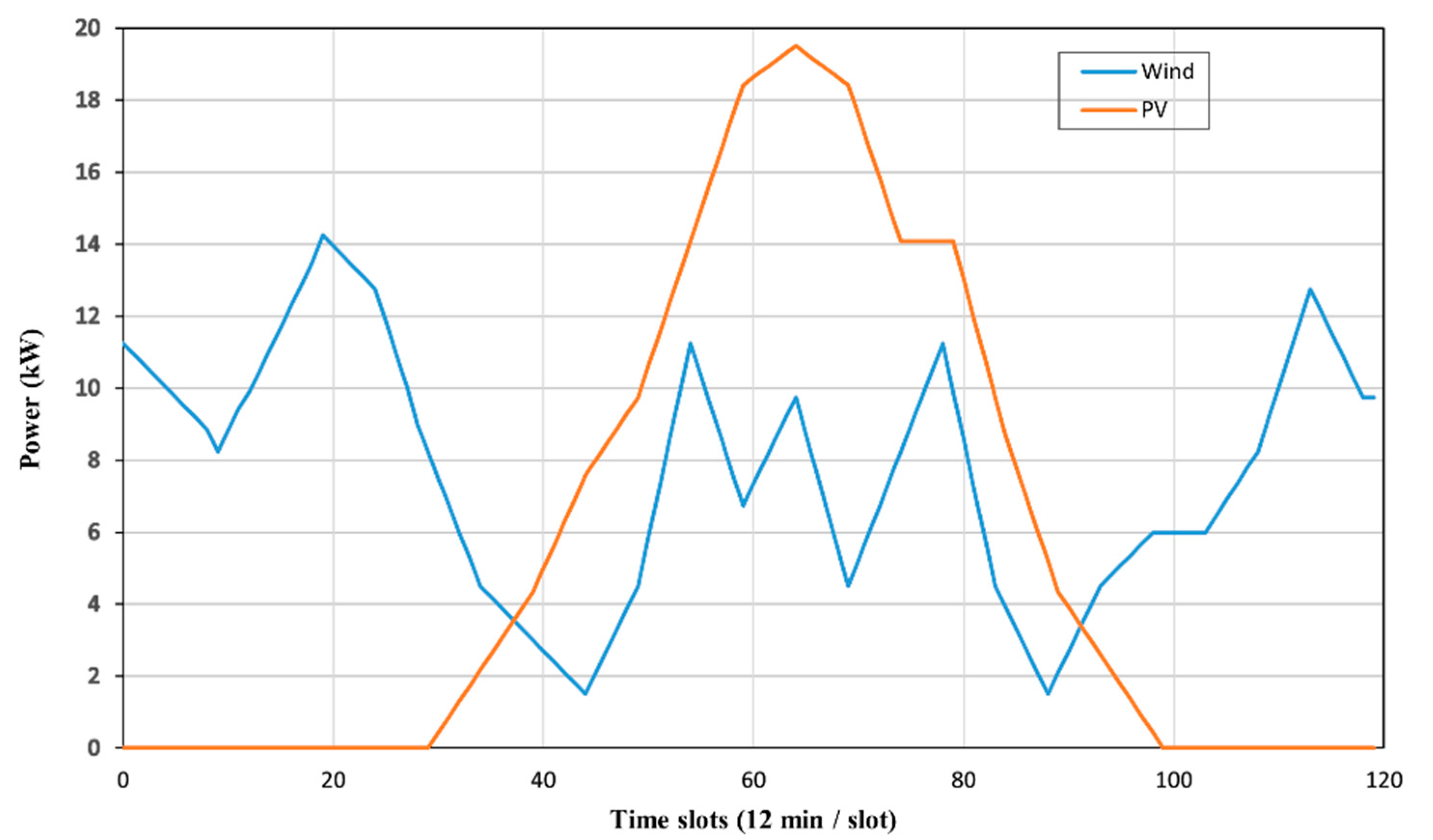
In this section we present the simulation results of the proposed algorithm for load power scheduling in the IMMG system. The simulation results were obtained using MATLAB R2019b software with a system having specifications of a 2.4GHz Intel core m3 processor with 8 GB of installed memory. A generic profile of PV, wind, and biomass power was used for RER data as shown in Figure 3. 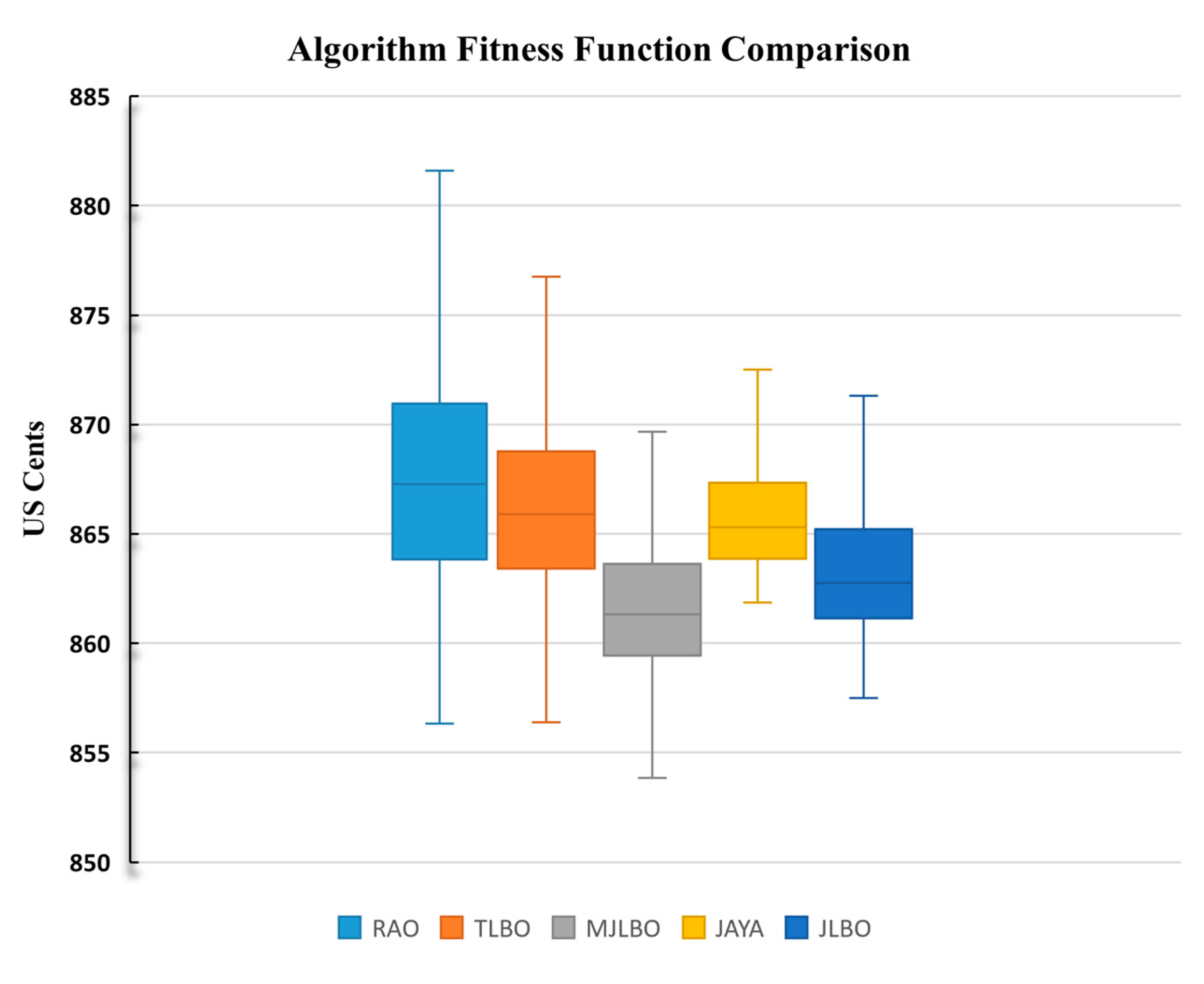User-defined slots and load power presented in Table 1 were used as the load for optimized scheduling. In order to check the effectiveness of the proposed algorithm, it was first compared with the other algorithms discussed in the literature. The effectiveness of the proposed algorithm is verified by comparing the fitness function values of 1500 iterations with the JAYA, TLBO, JLBO, and RAO as shown in Figure 7. The best, mean, and worst fitness function values for each algorithm are summarized in

Table 6. Fitness function comparison for 1500 iterations.

Algorithm	Best (¢)	Worst (¢)	Std. (¢)	Mean (¢)
RAO	856.318	884.9035	5.312024	867.4127
TLBO	856.3945	884.3665	4.770697	866.6044
MJLBO	853.861	884.7835	4.592001	861.8659
JAYA	861.8545	884.9695	3.85811	866.2355
JLBO	857.494	884.8615	3.974585	863.6717

. The illustration of the scenario configurations is demonstrated in

Table 7. Illustration of scenario and configurations.

Scenario #	Mode Description/Configuration
Scenario 1	Unscheduled load
Scenario 2	Scheduled load
Scenario 3	Scheduled load with increased BESS size

, respectively.

5.1. Comparing Gross Revenue in Local Electricity Transactive Method

Multiple simulation scenarios are discussed with various case results in this section. In each case scenario, five different gross revenue are calculated for a comparison of the proposed local electricity transactive method with the traditional power market. The first case indicates the net revenue of each microgrid when the prosumers do not undergo the market clearing process. In this case, the prosumers sell and buy electricity at national grid-defined tariff rates. This case will serve as the base case indicating the situation of the traditional power market for domestic prosumers. In case 2, all the extra demand and extra power from.by each MG is served mutually by other MGs participating in LETM at the market clearing price (MCP). In this case, it is assumed that all extra electricity demand and supply is fully utilized within LETM as there is always equal power demanded by LETM for extra power to the LETM.

Compared to case 2, in case 3, only the demand that can be served by the respective available power from other participating MGs is charged at MCP; the rest of the power that is not served is treated as load shed. Similarly, the surplus power that is utilized by LETM-participating MG is sold at MCP while the remaining surplus is treated as power to be curtailed. The results of case 4 represent the situation for a future perspective when the IMMG also integrates with the utility grid. The gross revenue is calculated using two different tariffs; one cost is calculated for the amount of power demand that is served just by the other MGs based on the MCP and other cost is calculated for the remaining power that will be served by the utility grid at its export tariff. Similarly, one gross sale is calculated for the extra power that is utilized by other MGs at MCP and remaining available surplus is sold to the grid at its own import tariff. Here, it is assumed that grid export tariff price is greater than the tariff of each participating MG and similarly, the import tariff of the utility grid is smaller than the MCP to maximize the participants involvement in the LETM. The gross amount in case 5 is for when the export tariff of each MG is same as its self-catered tariff described in aforementioned Table 3 (under Section 2.2.8 titled Modelling of Electricity Tariff).

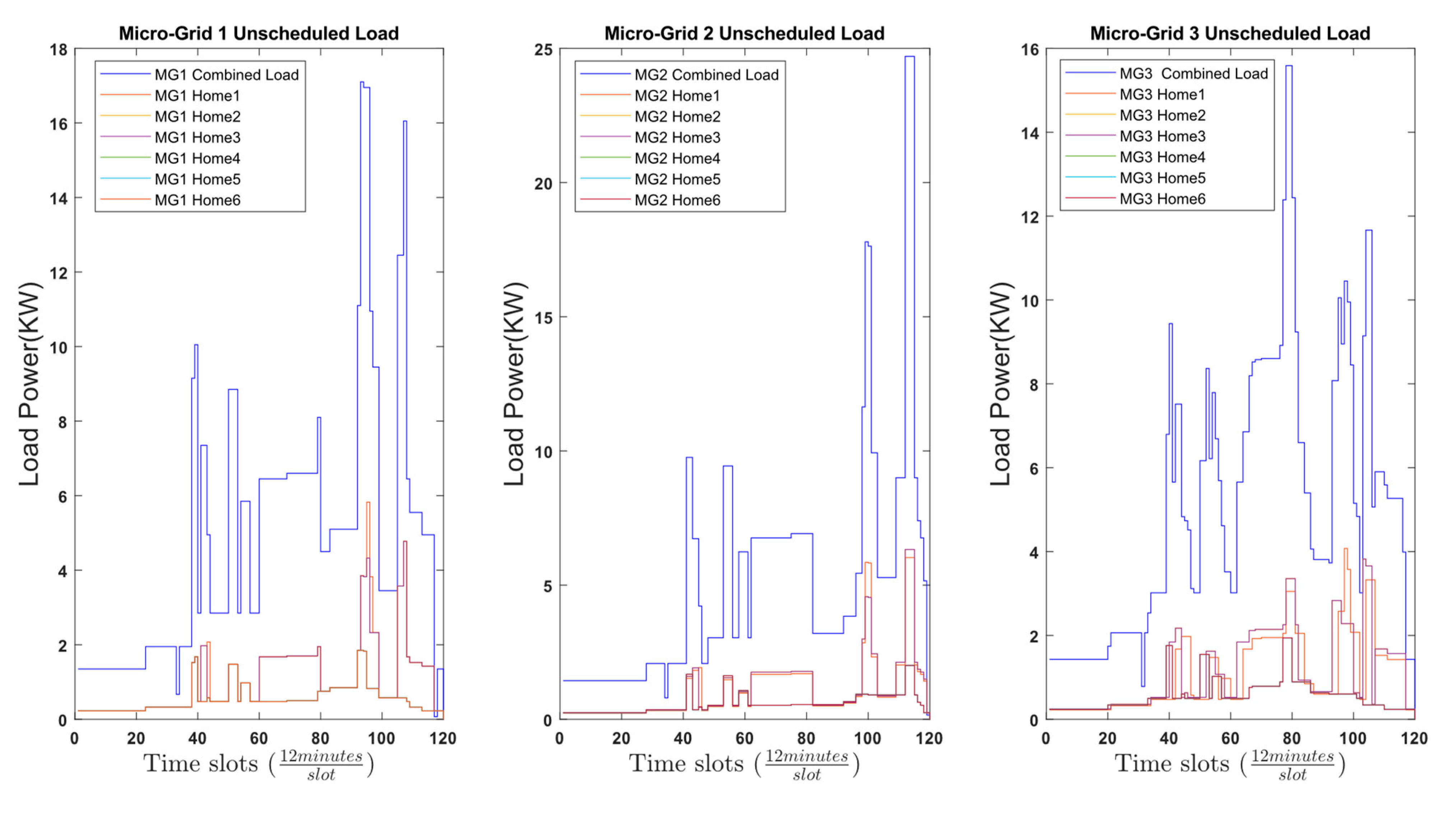
5.2. Scenario 1: Unscheduled Load Mode

In this scenario, the prosumer randomly selects the time position of the appliance to start the operation between the starting time and ending time range. The time slot range in this scenario is fixed as presented in Table 2; however, the load scheduling is not optimized. The total best total gross cost of electricity for the base scenario with case 2 revenue is −9.1768¢ per day (MG₁ = −126.932¢, MG₂ = −92.3638¢, MG₃ = 210.1192¢). The positive value indicates that the respective MG will have to pay for electricity. The results of this scenario will serve as the base reference for other scenarios as summarized in

Table 8. Gross cost for five cases of unscheduled load with fixed time slots.

MG #	Gross Cost 1(¢)	Gross Cost 2(¢)	Gross Cost 3(¢)	Gross Cost 4(¢)	Gross Cost 5(¢)
MG1	−324.489	−138.826	−126.9322	−296.215	−58.6855
MG2	−608.4513	−298.8426	−92.3638	−514.4684	−315.2225
MG3	219.0164	444.6284	210.1192	321.761	452.305

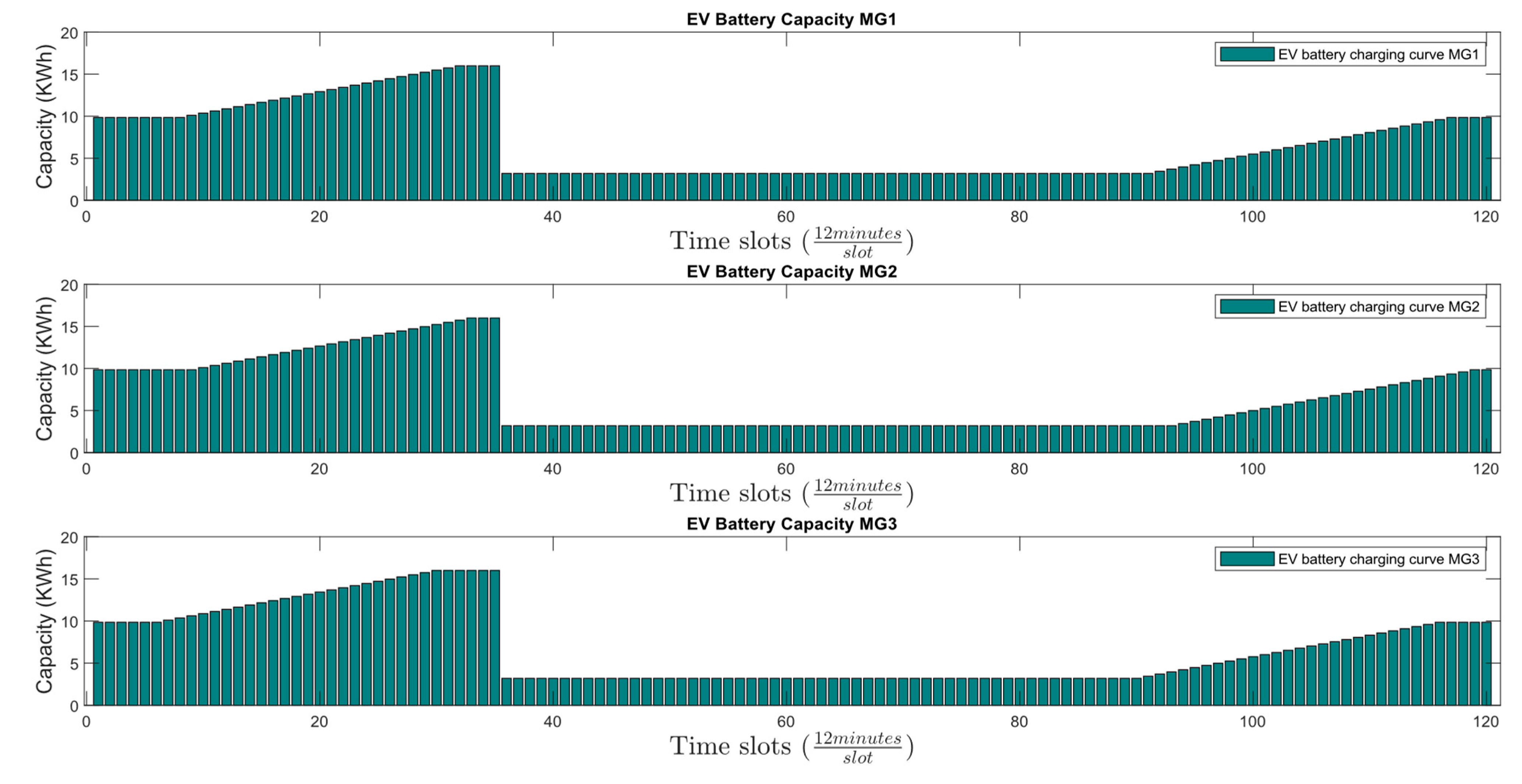
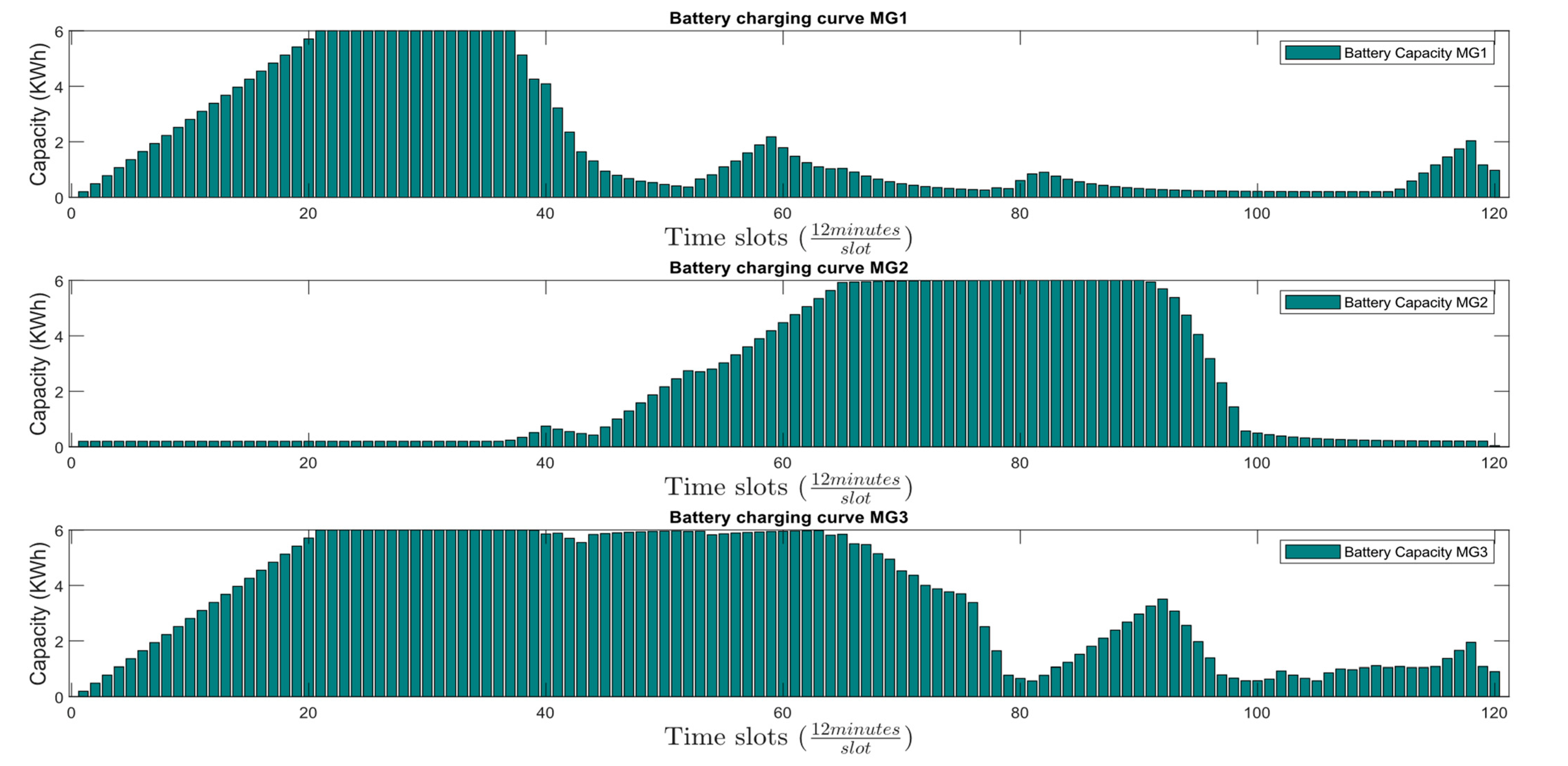
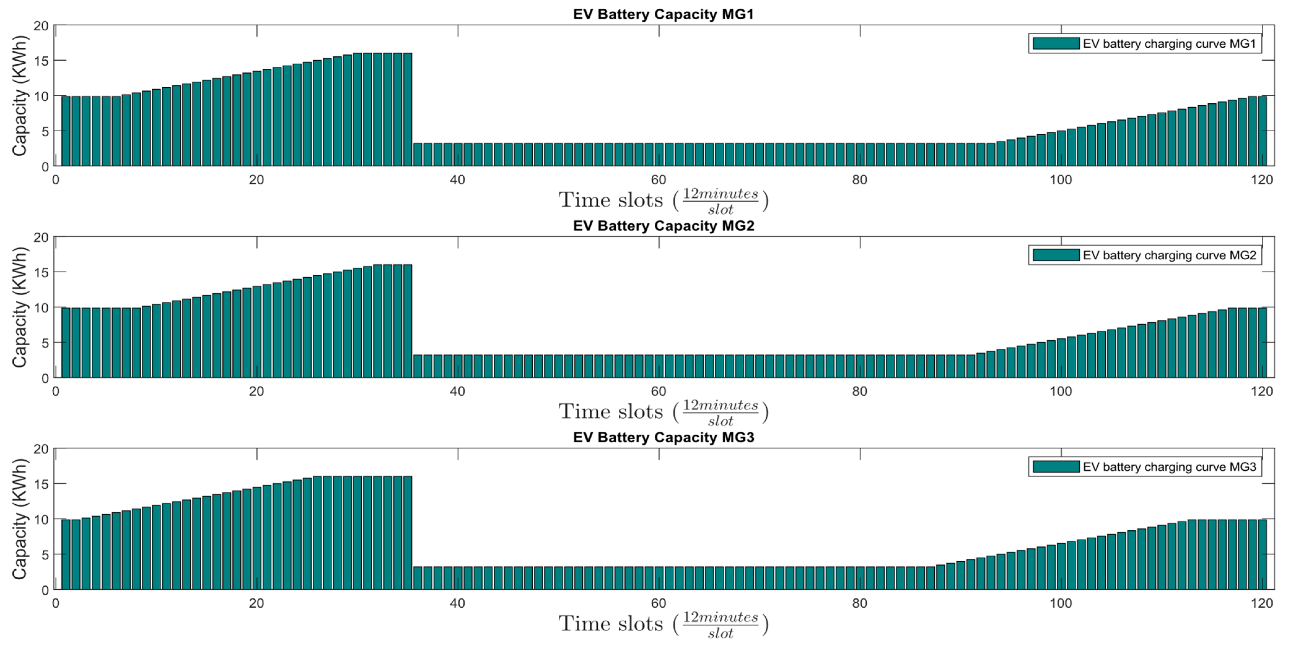
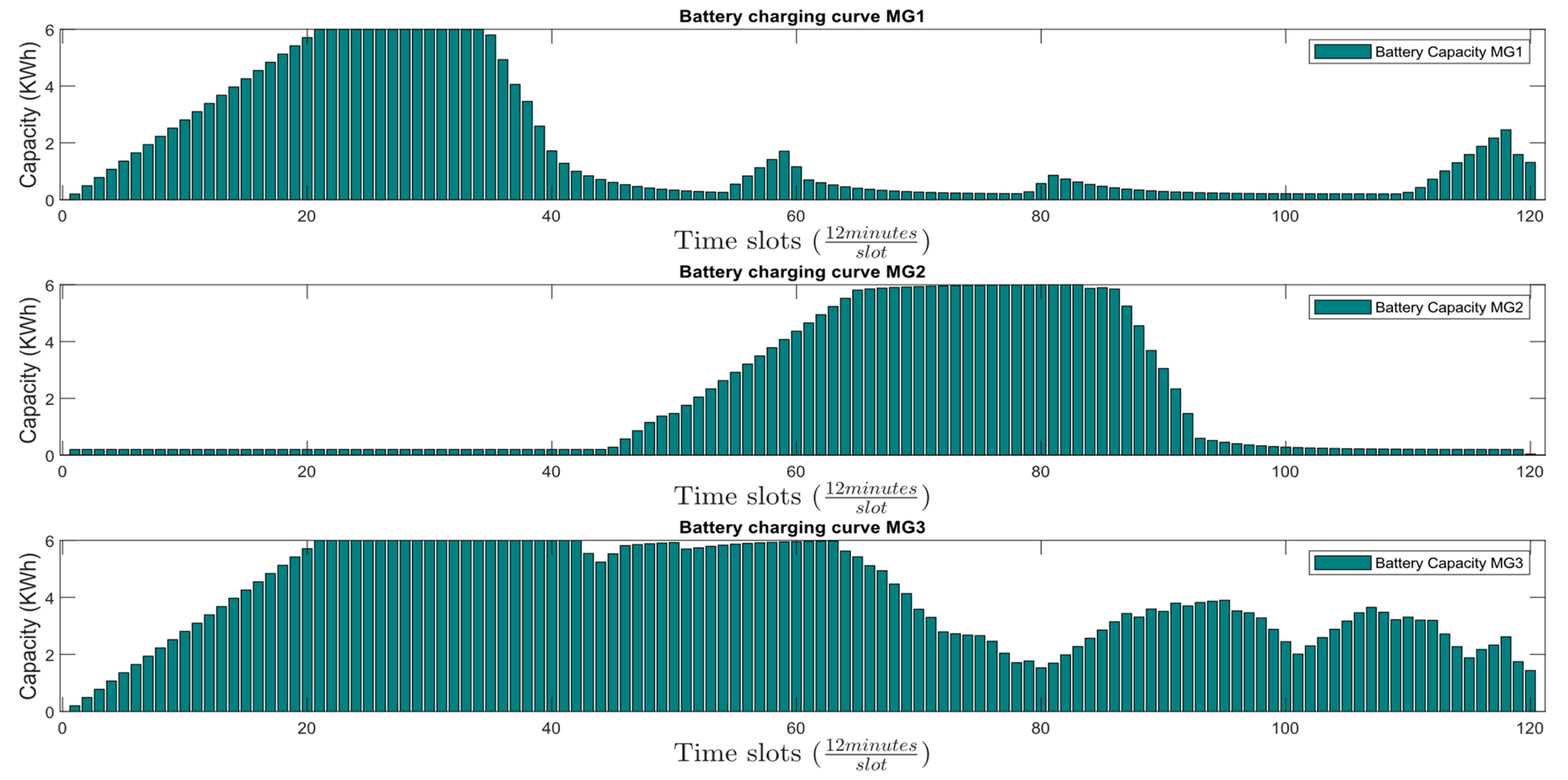
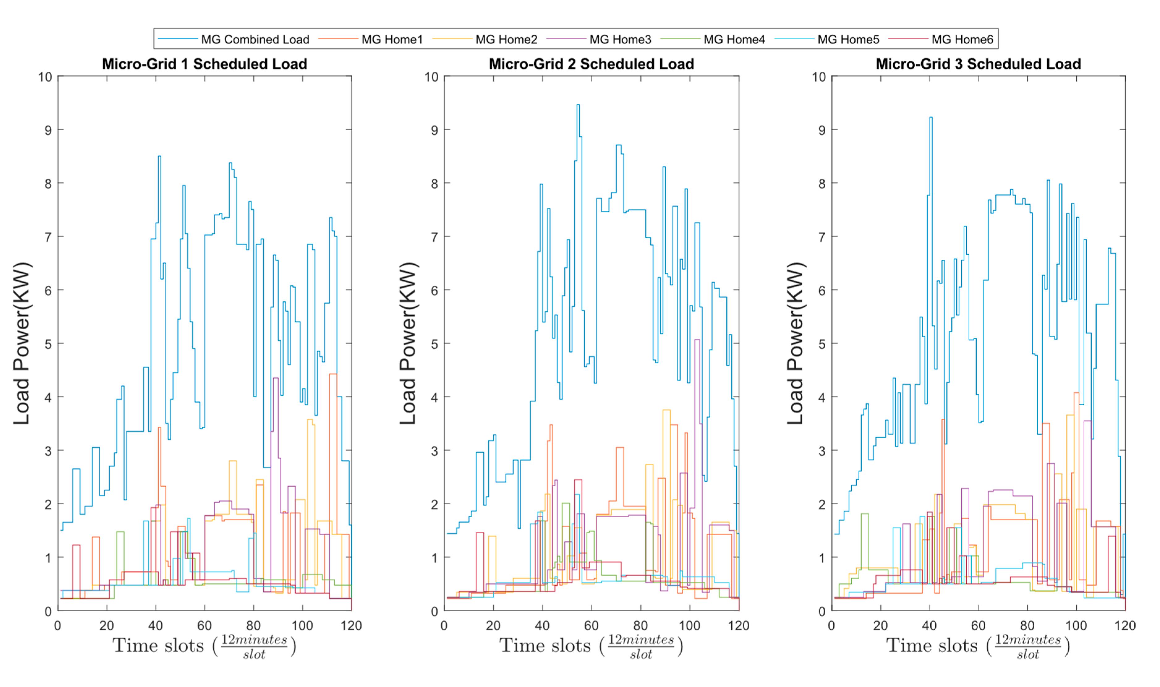
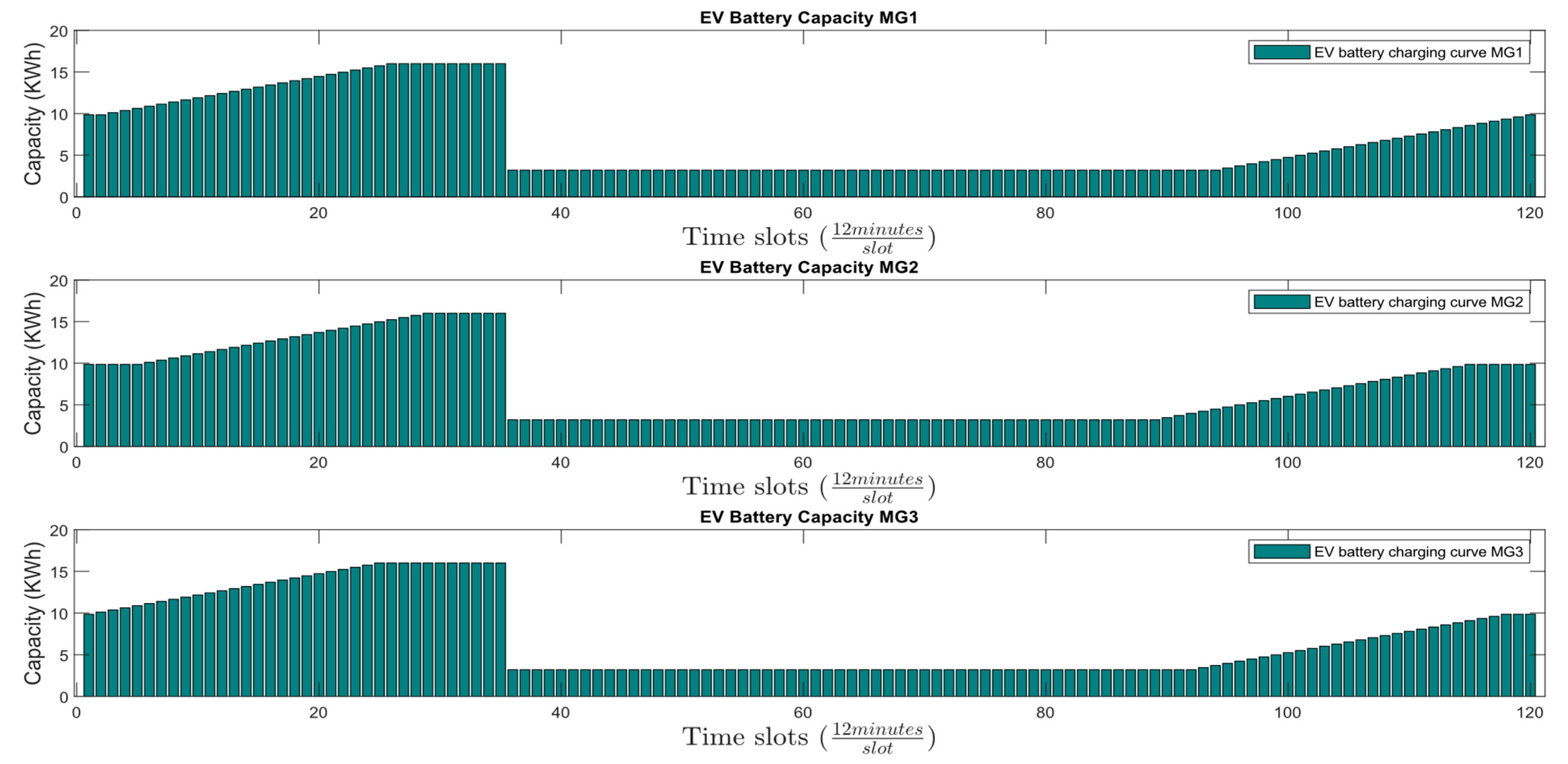
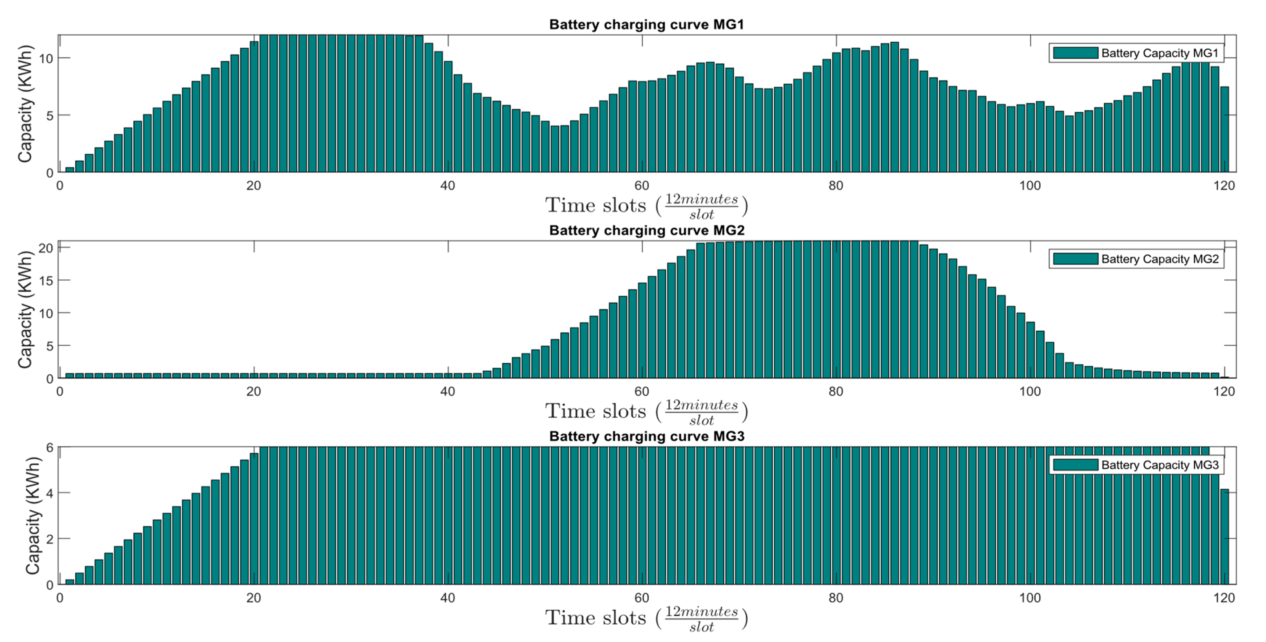
. The positive cost for MG₃ indicates that it earned the money by selling electricity. This is due to the fact that biomass power is modeled on the base of a constant power source will have less power fluctuations as compared to the stochastic nature of the other RER. Figure 8 shows the unscheduled load demand of each MG with individual homes. A slight variation in the starting and ending slots of each home is done for variation in the load curve of each MG. The capacity curve of the EV battery and BESS is shown in Figure 9 and Figure 10, respectively. The EV battery is modeled to be charged in 50 time slots throughout the night to reduce the cost and peak demand on grid.

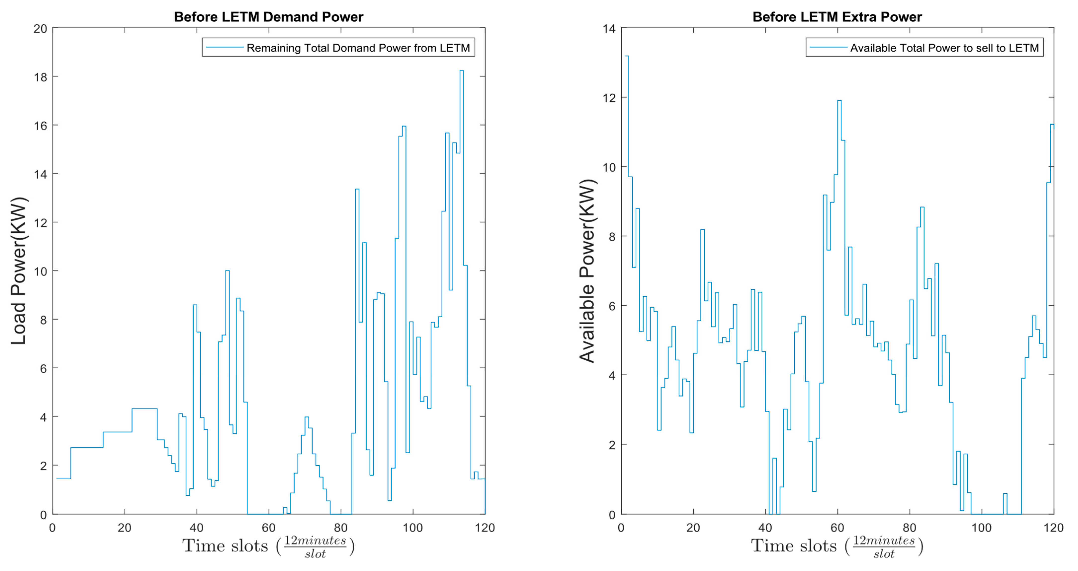
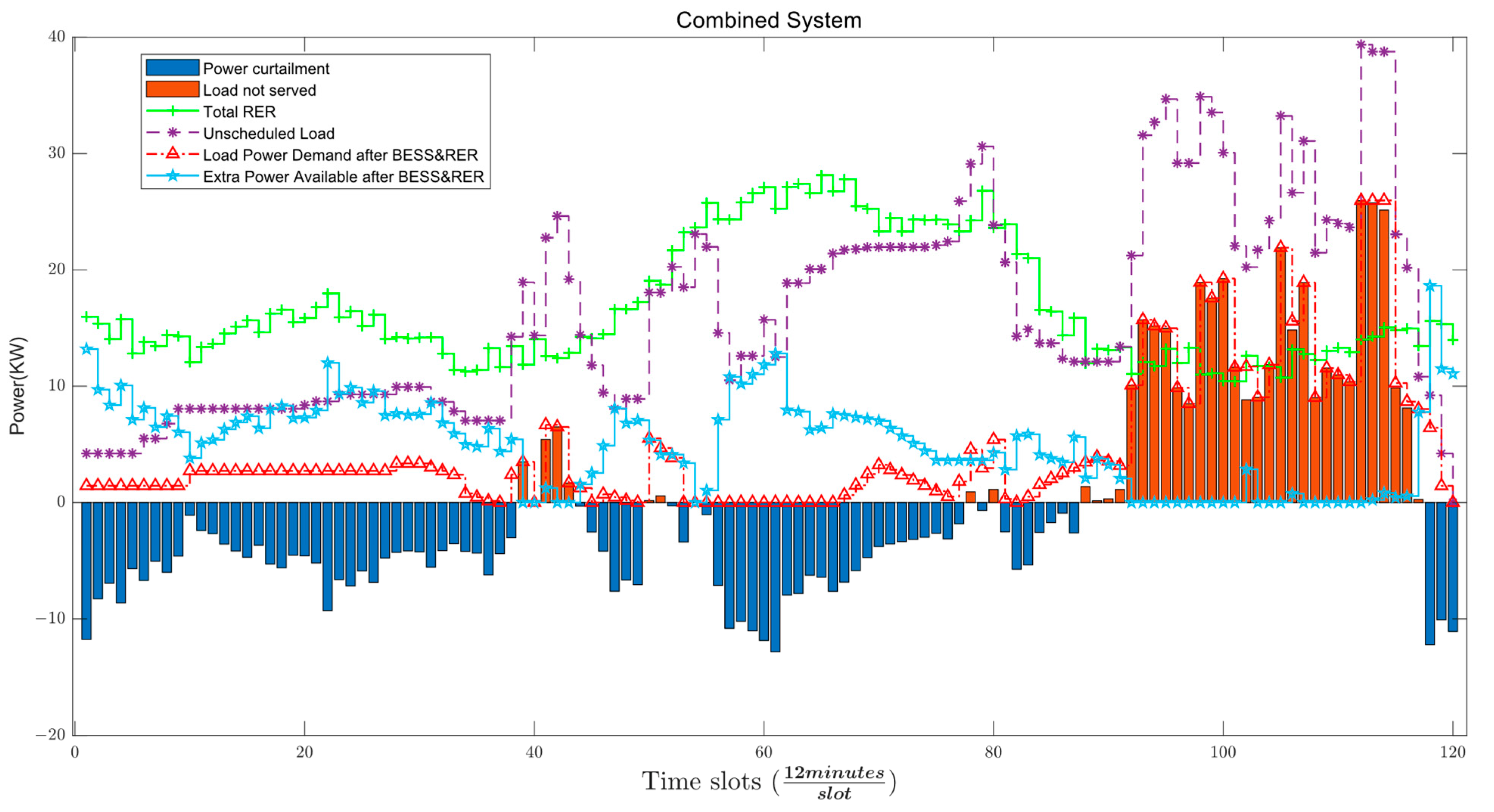
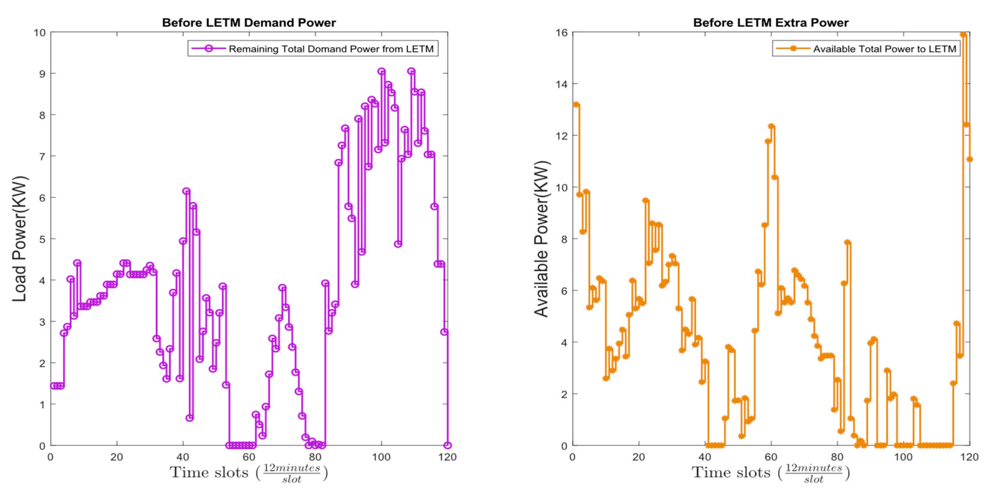
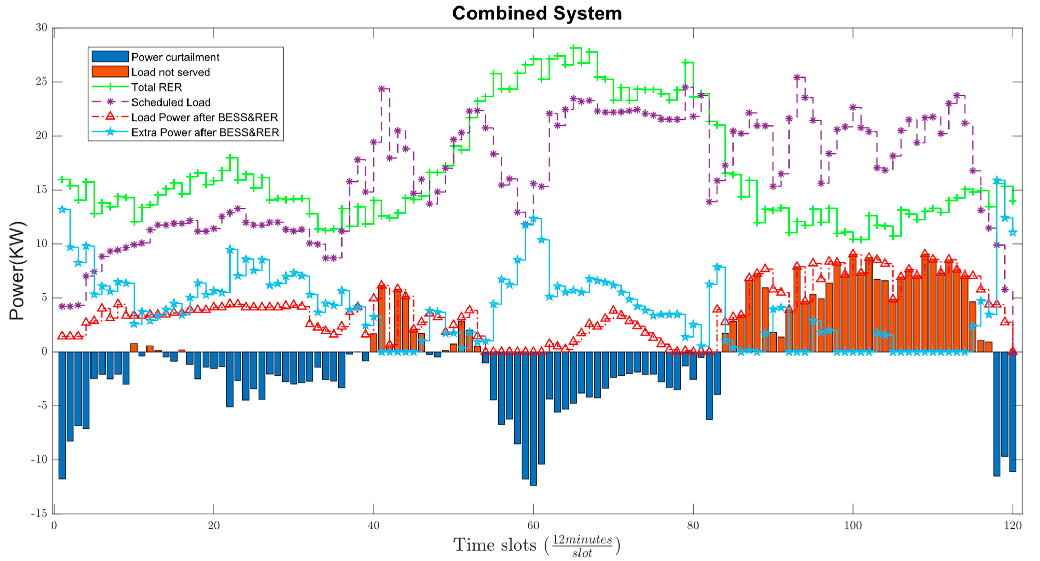
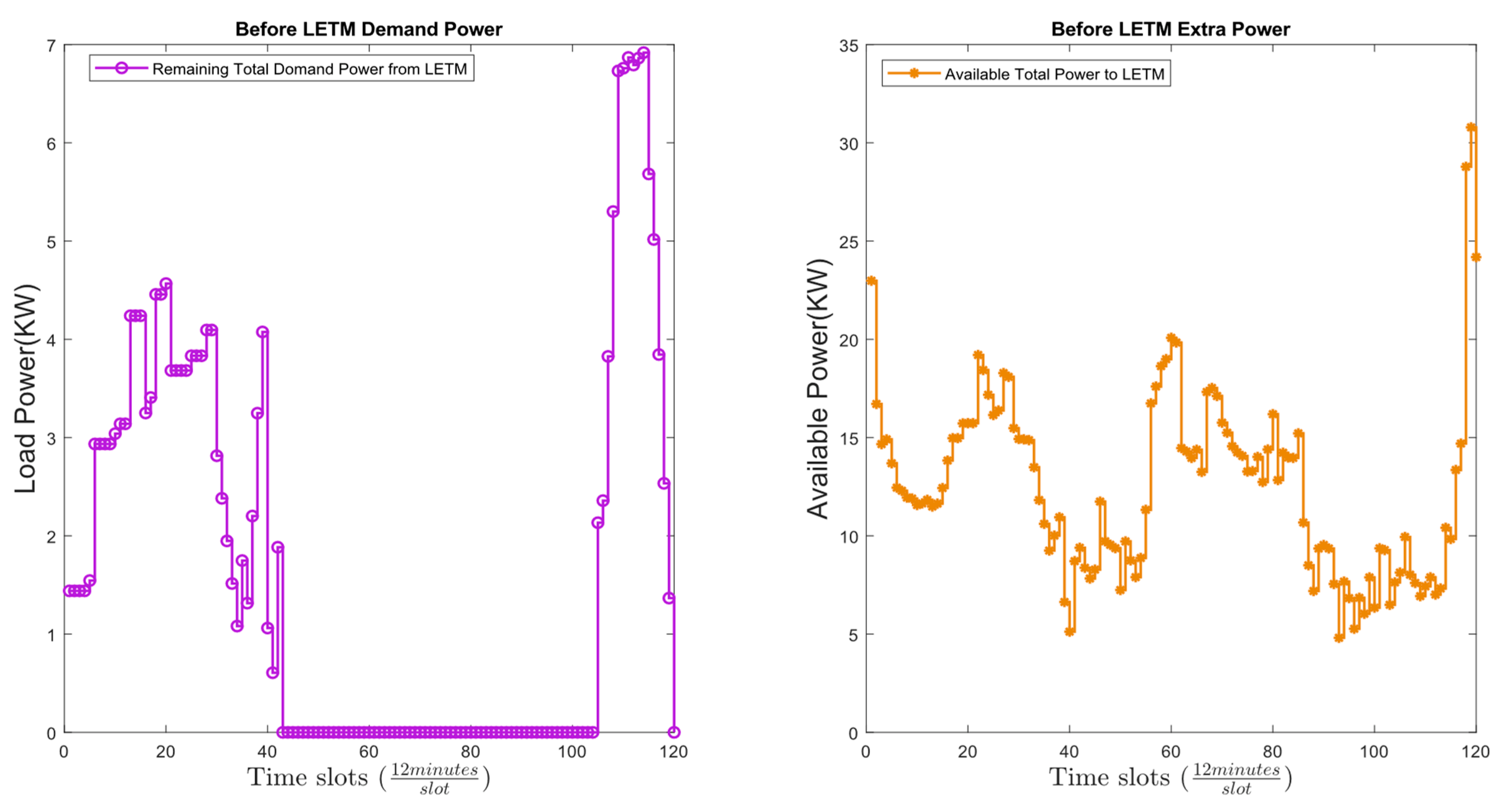
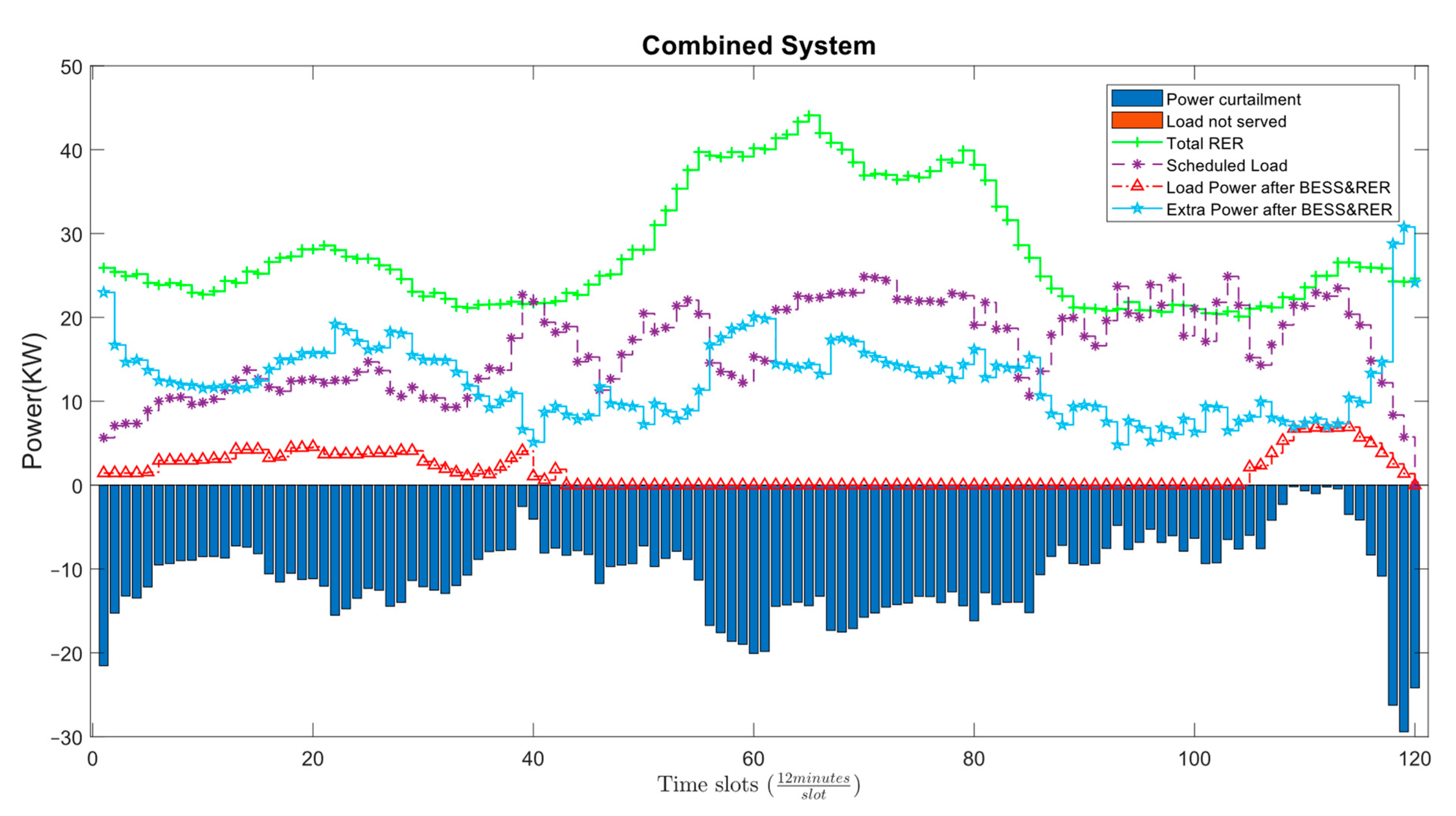
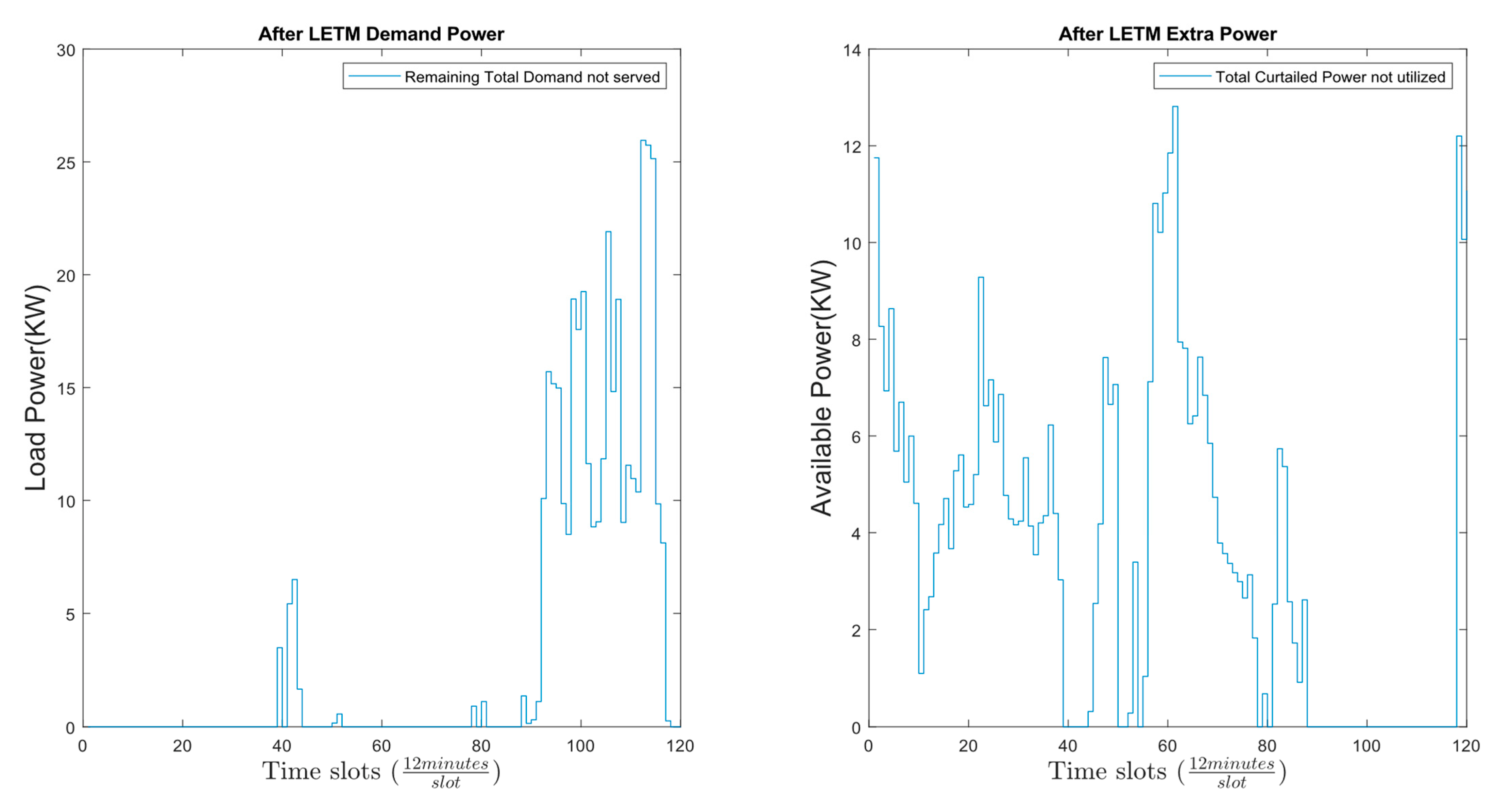
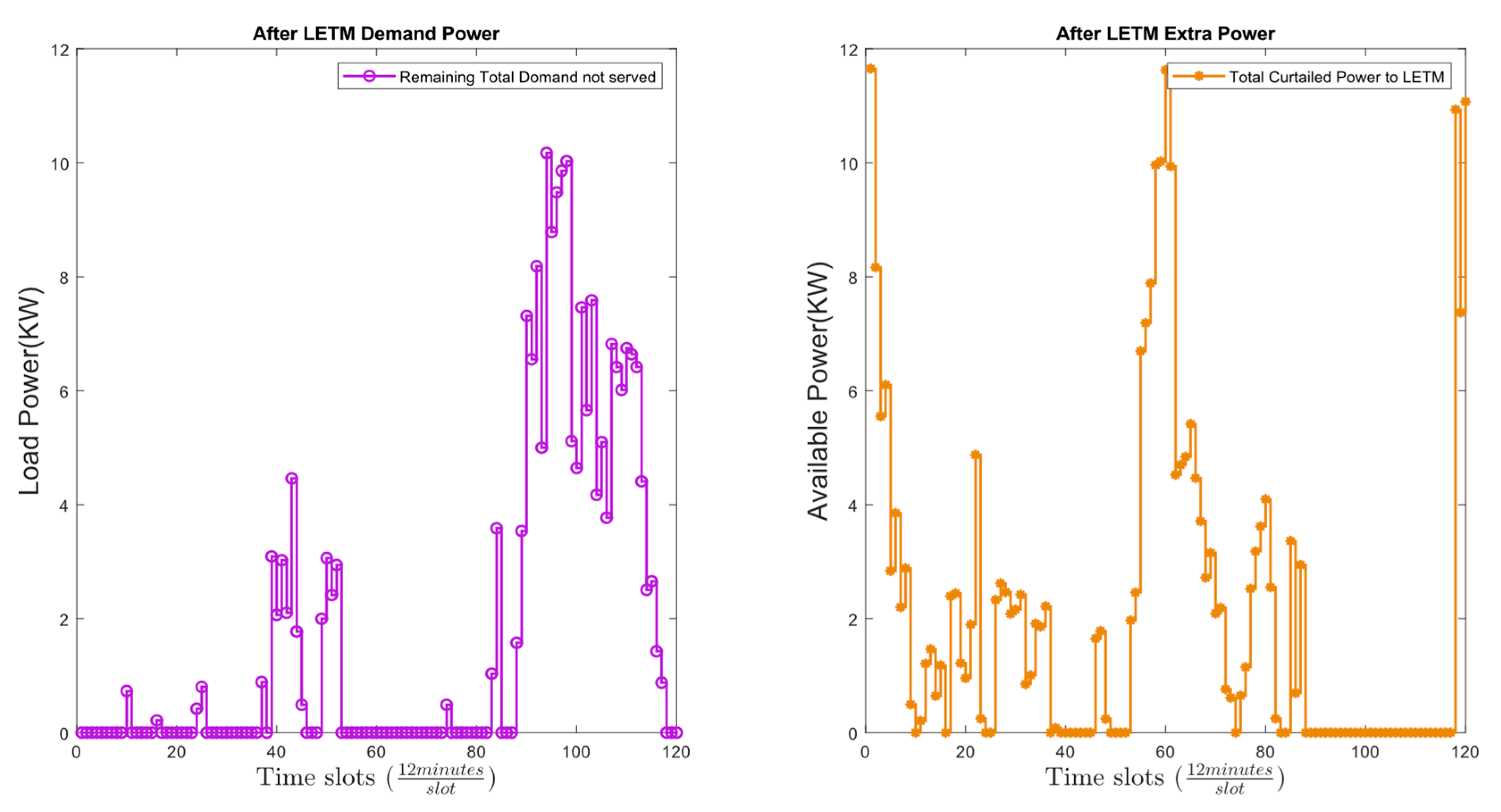
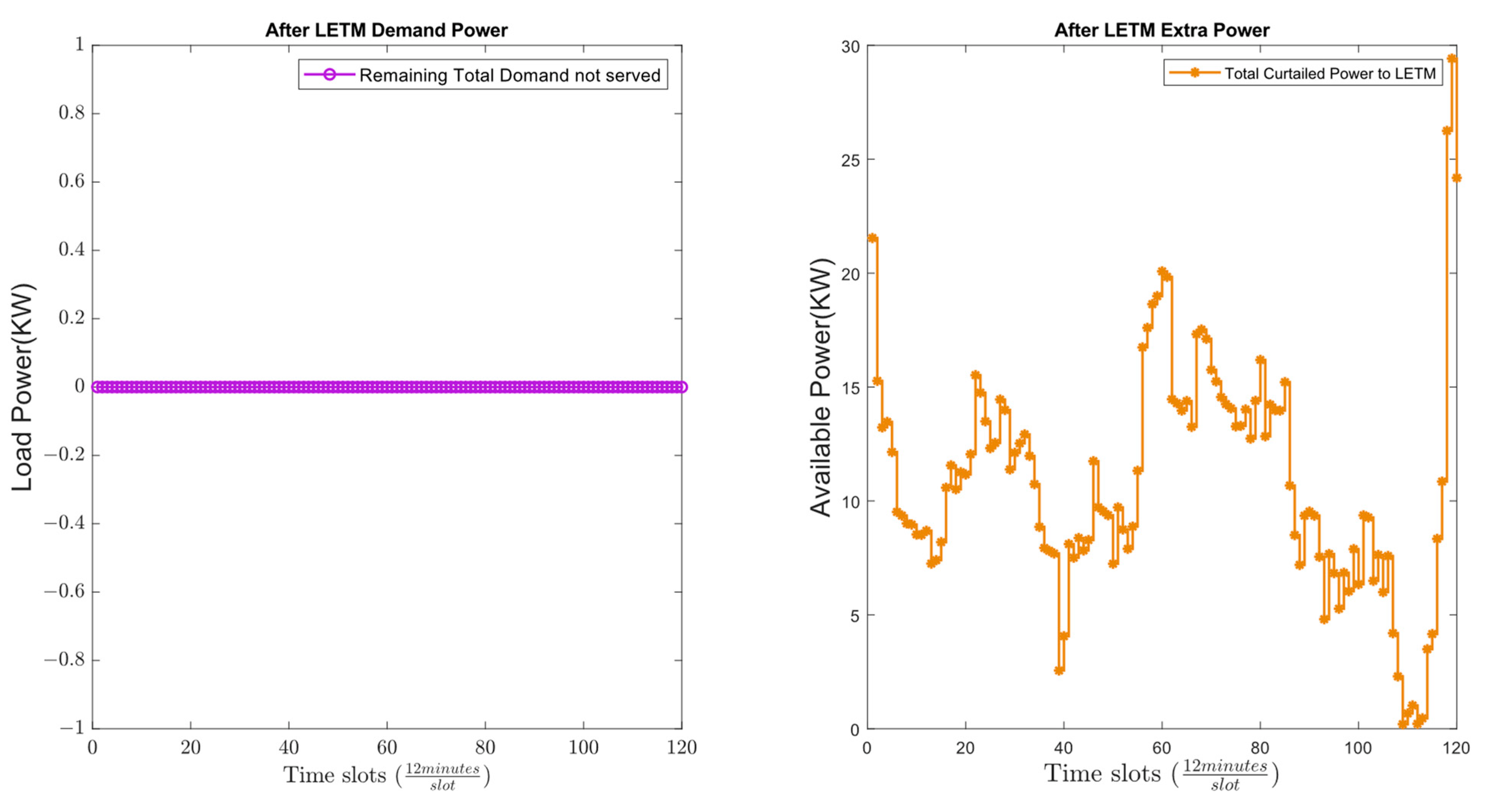
The total load power remaining after the RER and BESS taken from the LETM and the total surplus power of each MG after serving its respective load is given to LETM where other MGs will be participating. The total demand and surplus power before are shown in Figure 11 and similarly the remaining power demand and surplus which cannot be served by the IMMG system are represented as load shedding and power curtailment as shown in Figure 12. 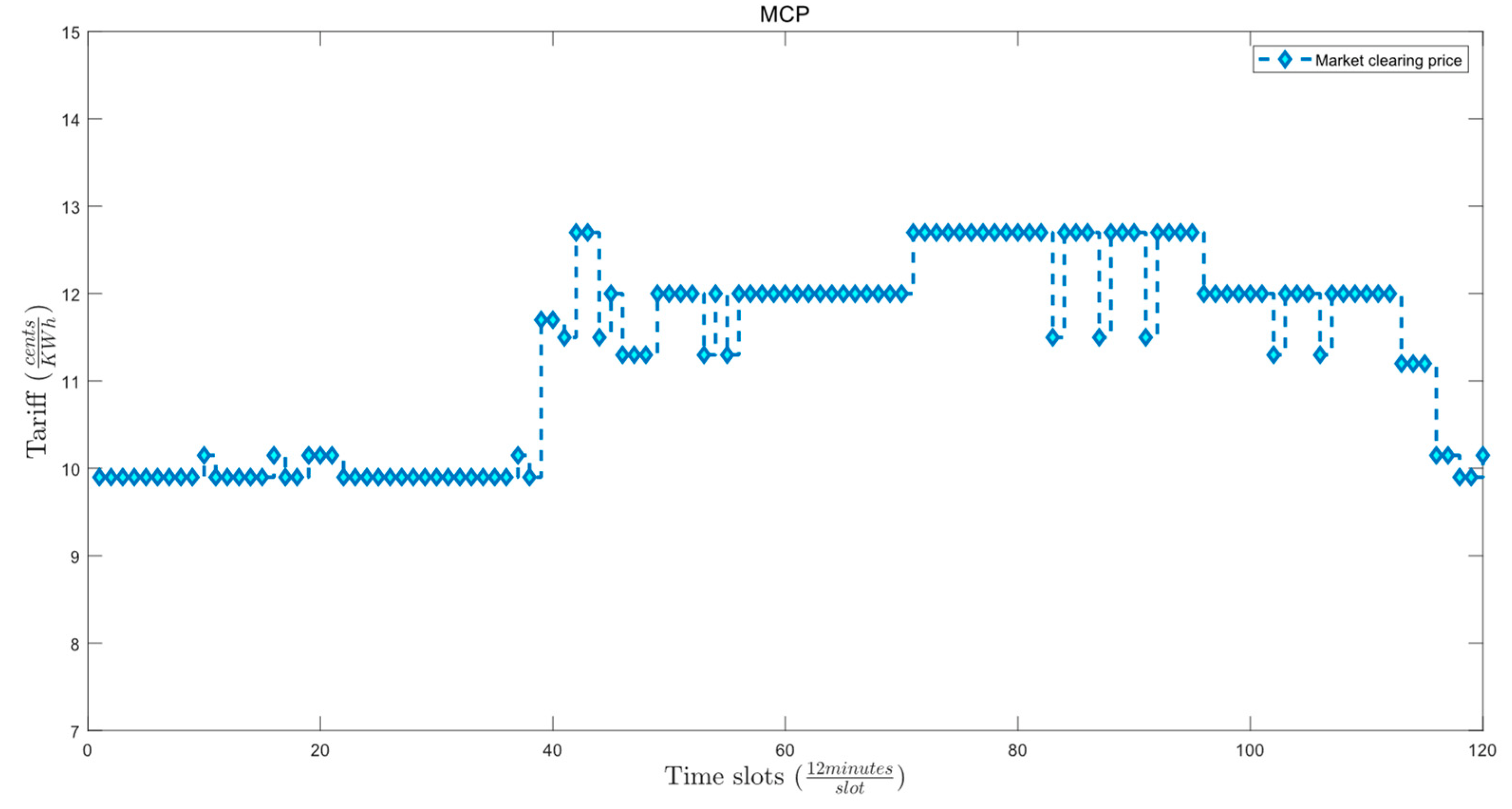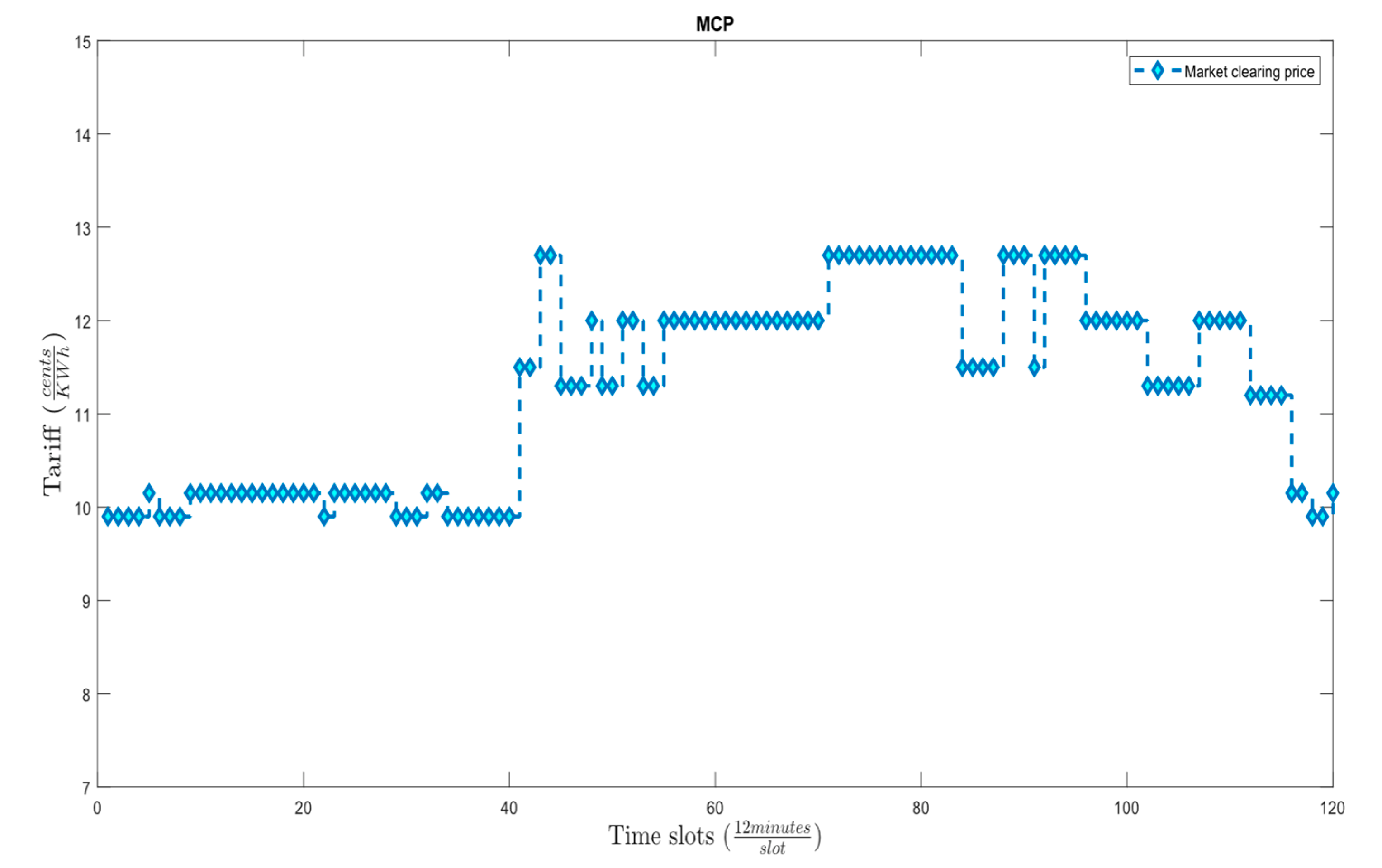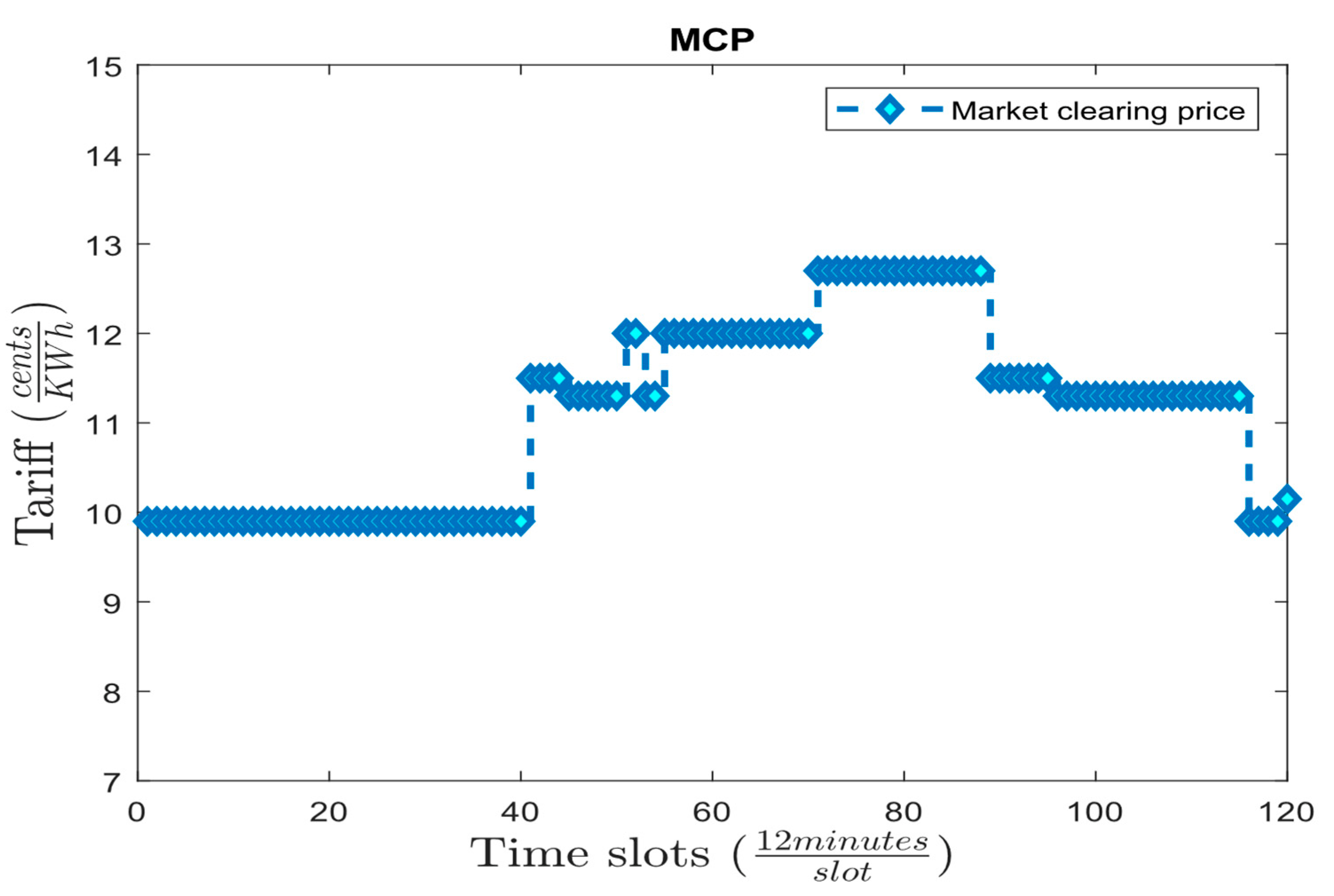Figure 13 shows the MCP set by LETM for energy buying and energy selling to the participant MGs in LETM.

Figure 14 shows the simulation results of the energy management system for the unscheduled load scenario for fixed time slots. The total energy demand of the whole day for the proposed network is 380.94 kWh while the total energy produced by RER is 404.94 kWh. The net energy demand before and after LETM is 112.162 kWh and 77.367 kWh per day. Similarly, the net surplus energy before and after LETM is 120.162 kWh and 86.367 kWh per day. A total of 31% of requested load demand is served by LETM and an energy curtailment of 86.035 kWh happens in the LETM. An overall 79.6% of total energy demand is served and 78.7% of the total available RER is utilized in the base case. This extra energy curtailment is due to the extra power being available at an instant when no power is demanded from LETM. Since the PV power is only available during the daylight, the load of PV-dominated MG₂ is served by the other MG.

Similarly, the first peak occurs at the time slot interval 35–45 as the operating time window of most loads is defined in this range. During the daylight, in the time interval 50–80, PV-dominated MG sells most of the extra electricity while charging its battery. During the nighttime, PV power is not available and the power output of the wind RER reduces and the load is either served from the stored energy in the batteries of the respective MG BESS or the biomass RER. Since all the loads in the proposed works are assumed to be uninterruptable and the EV batteries’ charging time is from time slot 85–120 and 0–120, this load power of the combined MG which cannot be served by BESS and LETM is thus shown as the load demand not served in Figure 14.

5.3. Scenario 2: Scheduled Load Mode

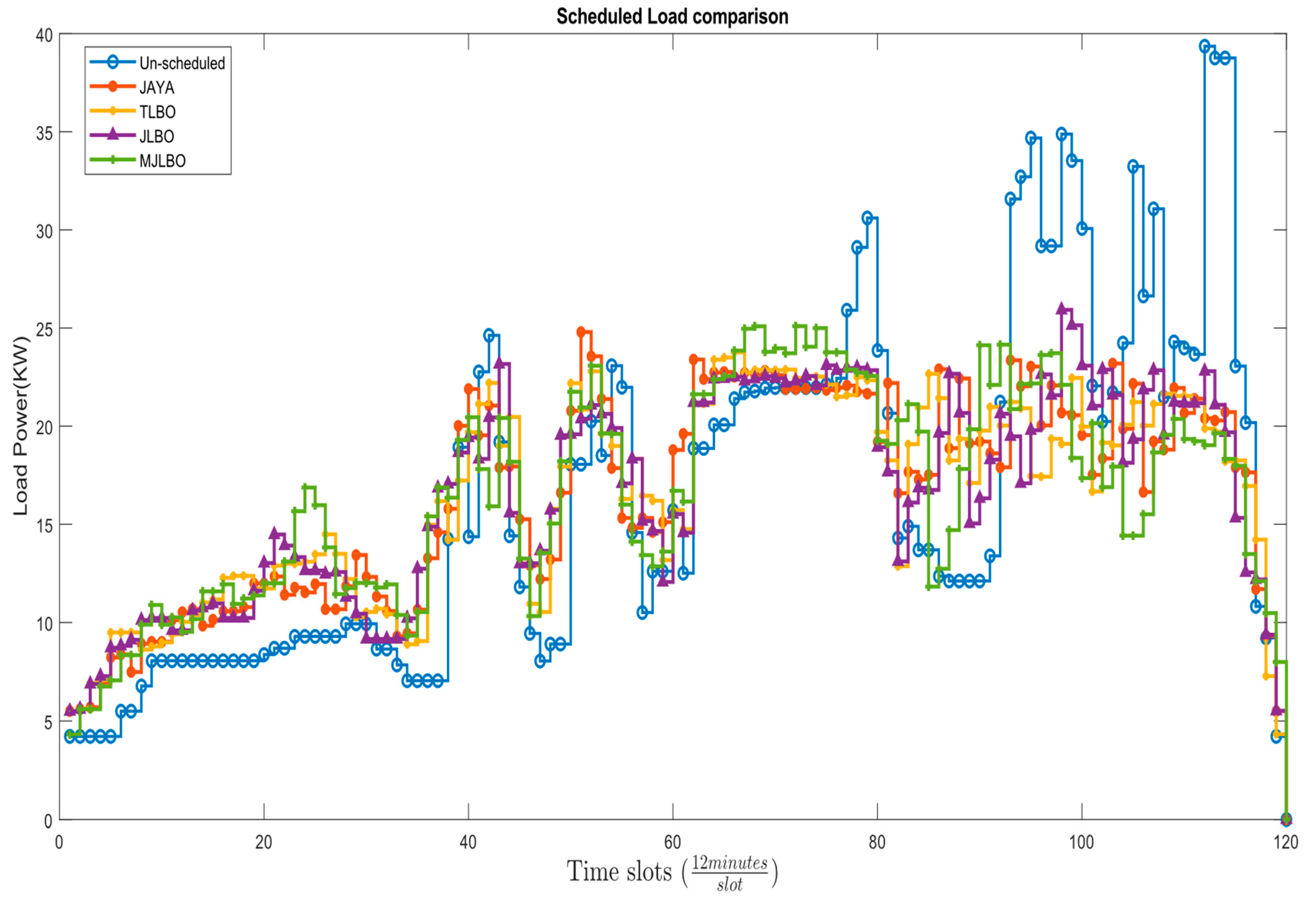
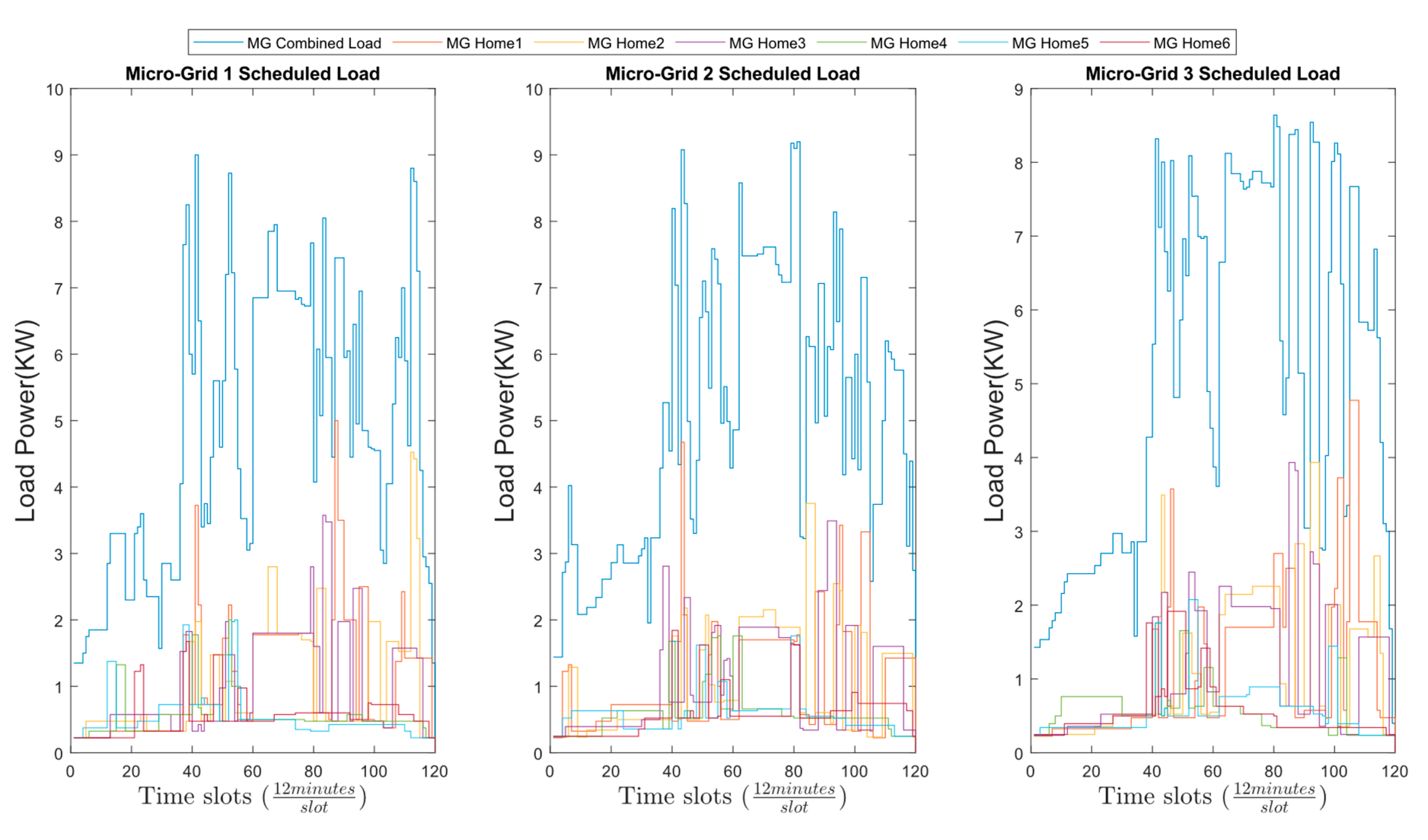
In this scenario, the starting position slot of each load is stochastically selected within the operating time window using Equations (14)–(16) by the algorithm. The best combination of appliance operation is selected to minimize the MG electricity cost and PAR while simultaneously keeping a minimum user discomfort by allocating load appliances to appropriate time slots. The per-slot load comparison of the proposed algorithm with unscheduled and other algorithms such JLBO and JAYA is shown in Figure 15. The peak demand in case of unscheduled load reaches 39.36 kW while for the scheduled case, maximum demand occurs in the JLBO algorithm with the peak reaching 25.93 kW. In the case of MJLBO, the peak value is 25 kW and the lowest peak value of 23.76 kW occurs in the case of the TLBO algorithm for slot 66.

In all cases, there is a peak reduction of more than 34%. Most of the loads are scheduled at dawn and dusk time as high-power loads are stochastically allotted at the slots where prices are low. During the time slot of 75–95, the prices are high but the prosumer defined window constraint bound the load to be operated in these time slots. During this peak time, in slot 35–45 and slot interval 75–95, MJLBO shifted some load to reduce the overall cost of electricity. The scheduled EV battery and BESS capacity curves are shown for MJLBO in Figure 16 and Figure 17.

Compared to scenario 1, the capacity curve of BESS shows a wider spread of battery utilization during the evening period and daylight. The energy in respective batteries of MGs is stored during time slots when the load demand of the respective slot is fulfilled and is discharged during high demand periods. MG₃ BESS is being utilized during the peak slots of 75–95. Similarly, MG₂ BESS is delayed for 2 h during slot 90–100 so that stored energy can be utilized for charging EV battery and other loads at night. Figure 18 shows the per-slot load curve for the scheduled MG which shows the load is distributed throughout the day to reduce the peak while concurrently minimizing the electricity cost and discomfort.

The results of the LETM on load demand and surplus power for each time slot are presented in Figure 19 and Figure 20. It can be observed that the combined load peak in the LETM scenario is reduced by 60% compared to the scenario without scheduling. However, the surplus energy generated during the noon time slots was not fully utilized by the participating microgrids (MGs) due to the scheduling of high-power appliances for operation during the afternoon and night time.

As a result, the PV-dominated MG₂, which is unable to supply the load during the nighttime, was only able to meet a fraction of the load demand using its BESS. The remaining load demand had to be fulfilled by other MGs, with the more stable biomass-based RER in MG₃ shouldering a sizable portion of the load during the time slots 85–95. This period also saw a reduction in the power supplied by the wind-dominated MG₂. Therefore, the load demand which cannot be fulfilled during the slots 95–110 appeared as a load that needs to be shed. Contrary to this, during the start of the load curve, there is enough surplus energy in MG₂ and MG₃ to charge the EV batteries. Again, during the morning peak demand time, surplus energy is not enough in the LETM and a peak of 4.3 kW appears on the load curve during the 40–44 time slot interval.

Figure 21 shows the MCP of scenario 2 which is very similar to scenario 1 as, in both cases, MCP is determined by the MG which can provide the highest price but the least amount of power which is for the MG₂ so that each MG can have an optimal cost with maximum power demand served by LETM. The complete EMS for the whole day is shown in Figure 22 for the scheduled load in fixed operation time slots. Compared to scenario 1 where only 31% of total daily energy demand was served and 71% of surplus energy was curtailed by the LETM, in this, more than 53.4% of demand from LETM-participating MG was served while 50% of surplus energy had to be curtailed. Thus, a significant effect of load scheduling on energy serving and optimal utilization can be observed.

Similarly, the simulation of scenario 2 for load scheduling using TLBO, JLBO, and JAYA algorithms showed that the LETM was able to meet 47.26%, 43.73%, and 46.65%, respectively, of the total daily energy demand, while curtailing 56.41%, 59.2%, and 56.5%, respectively, of the surplus energy. An overall 88.94% of total energy demand is served and 87.66% of the total available RER is utilized in this scenario using MJLBO. Similarly, an overall load serving of 87.32%, 88.12%, and 87.73% of the total energy demand of network is observed using JLBO, TLBO, and JAYA, respectively.

The total best gross cost of electricity for scenario 2 with case 2 revenue is 45.0759¢ per day (MG₁ = −122.1634¢, MG₂ = −285.634¢, MG₃ = 452.873¢). The effect of scheduling is evident from comparing the gross cost results of scenario 2 with the base scenario as shown in

Table 9. Gross cost for five cases of scheduled load with fixed time slots using MJLBO.

MG #	Gross Cost 1(¢)	Gross Cost 2(¢)	Gross Cost 3(¢)	Gross Cost 4(¢)	Gross Cost 5(¢)
MG1	−284.3605	−122.1634	−77.2371	−220.764	−60.4262
MG2	−546.7809	−285.6341	−246.9921	−433.738	−323.4525
MG3	267.1669	452.8734	315.0753	395.6741	445.4065

. Here, the net cost of electricity for the 100% LETM trading case is observed to be 45.07¢ per day as compared to 6.95¢ per day which means a total profit of 11.433$ per month for the whole IMMG system instead of going to the utility grid for 100% load and surplus energy utilization and paying 169.19$ to the utility grid. It is important to consider how energy demand and supply change throughout the day, or over different time periods, when designing and operating the LETM. This is because the demand for energy and the availability of surplus energy are at different time slots and can vary significantly at various times of the day, depending on the scheduled use of high-power appliances and the output of the participating microgrids (MGs).

5.4. Scenario 3: Scheduled Load with Increased BESS Size

In scenario 3, the load demand that could not be met during nighttime was due to insufficient BESS in the MG and a lack of renewable energy resources. As a result, the amount of RER power was increased by 50% in each MG, with a particular focus on increasing the size of the BESS in MG₂. This allowed for the storage of excess energy produced by photovoltaics during the day and its use to meet the load and charge electric vehicle batteries during later periods of the day. As a result, 100% load serving was achieved, but at the expense of increased electricity costs for users. The operation time slots for this scenario were similar to those of scenario 2 and remained fixed. The scheduled load in this scenario is shown in Figure 23.

In scenario 3, the capacity of the BESS in the MG and the EV batteries was increased, as depicted in Figure 24 and Figure 25, respectively. This allowed for a longer duration of surplus energy storage and backup power provision in time slot intervals of 90–110, compared to scenario 2. The BESS in MG₃ consistently maintained a charged state due to the abundance of RER available, which exceeded its load requirements throughout the day.

In MG_2, the surplus energy generated during high RER time slots was utilized to charge its BESS, enabling it to provide backup power to its respective load without fully discharging during the latter half of the day. This demonstrated the importance of increased storage capacity in isolated environments for meeting 100% power demand. It can be observed that all batteries were able to maintain a charged state for extended periods, emphasizing the necessity of a larger storage capacity to cover the entire power demand.

Before and after LETM power demand and surplus power are depicted in Figure 26 and Figure 27, respectively, indicating that the load demand is 100% met for the whole day. The increased amount of curtailment power in this scenario is due to the fixed starting and ending time slots defined for load appliances. The high demand during the time interval 105–115 is because the EV battery charging schedule is set to charge for minimum 5 h during the interval 85–120 and 5 h during the interval 0–35. The load during the first few slots is supplied by the energy stored in BESS in MG₁ and MG₂. The reduced amount of wind energy during the first half interval shifts the remaining demand on the MG₃ and its BESS. The sharp peak at the last slot of the day is due to the assumption that all BESS discharges and sells their stored energy to the LETM at end of the day and starts at minimum energy for the next day.

Figure 28 shows the MCP determined for this case scenario with a reduced average tariff price as compared to scenario 1 and 2. Figure 29 illustrates the complete energy management system for the scheduled load in fixed operation time slots with complete load serving. Compared to scenario 1 and 2 where only 31% and 53.4% of total daily energy demand was served by the LETM, respectively, in this scenario, 100% of demand from LETM-participating MG was served. However, this came with the price of increased curtailment of 87% of surplus energy and cost of electricity as the OM cost of BESS increased with the capacity increase.

The gross costs of electricity for scenario 3 shows that MG₃ had the highest revenue since its residents did not have to pay for any power demand because of the ample amount of surplus energy, and benefited from LETM by selling the surplus energy to the rest of the MG. Unlike this, the residents of MG₂ had to pay the cost of electricity since there is no source of energy during the start of the day until the sun shines for the PV system to produce power. Thus, it must buy the extra demand from other MGs to meet a 100% load demand. The five gross costs for scenario 3 for one day are summarized in

Table 10. Gross cost for five cases of scheduled load with fixed time slots with increased storage and RER size.

MG #	Gross Cost 1(¢)	Gross Cost 2(¢)	Gross Cost 3(¢)	Gross Cost 4(¢)	Gross Cost 5(¢)
MG1	266.0583	465.8583	−14.0278	275.0583	473.0583
MG2	−229.5764	83.0567	−451.0433	−152.5433	42.1774
MG3	1332.9694	2273.5694	369.6651	1486.9694	2219.2694

.

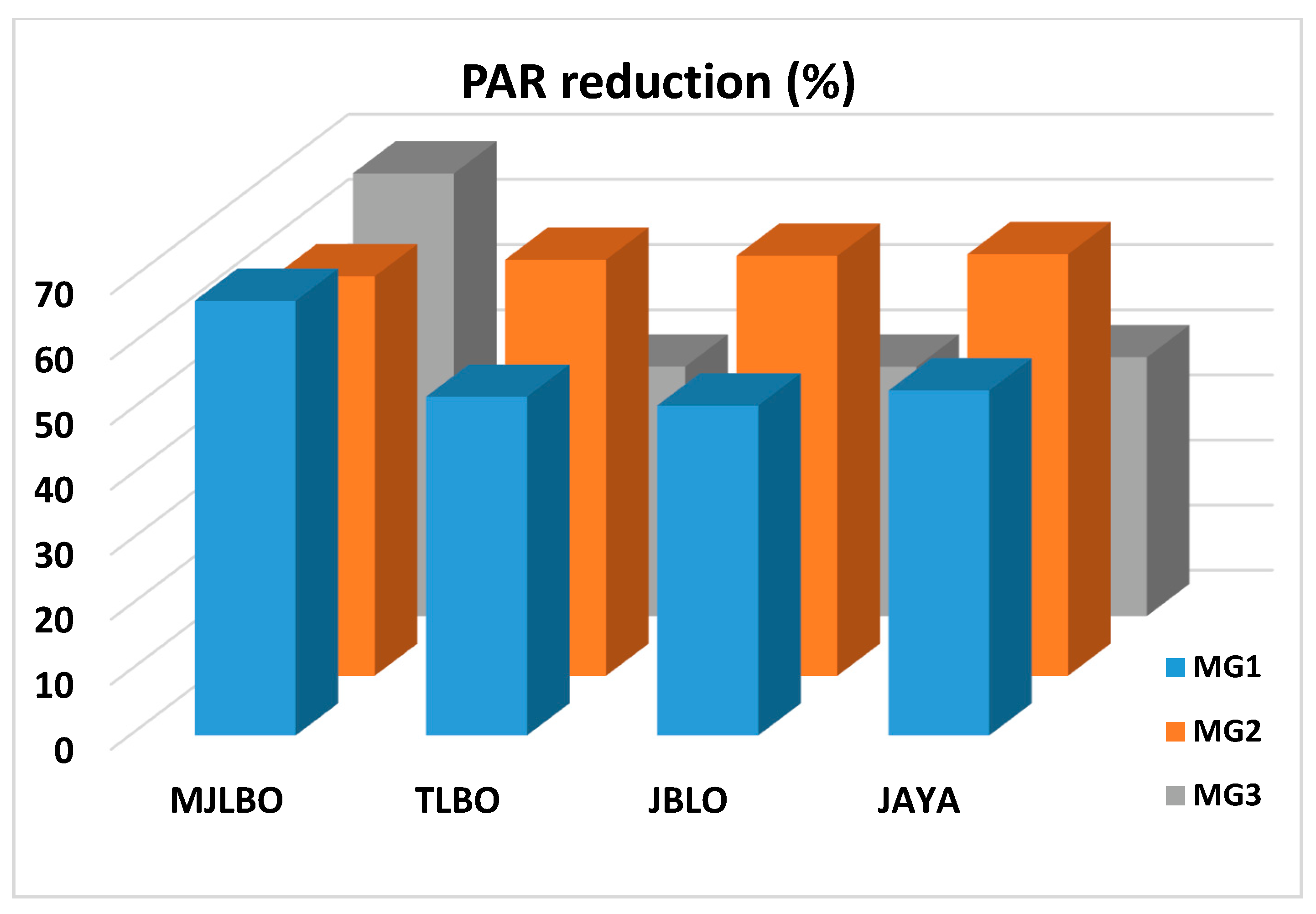
5.5. PAR Reduction

The PAR was reduced with the scheduling of load appliances. The highest peak reduction was observed with the proposed MJLBO with net PAR reduction of 65.38% and individually 66.8%, 61.37%, and 67.98% in MG1, MG2, and MG3, respectively. Similarly, the JLBO performed the worst with net PAR reduction of 51.2% with 50.76%, 64.52%, and 38.32% in each MG, respectively. The PAR reduction results in a comparison of other algorithms with the proposed MJLBO are summarized and observed in Figure 30.

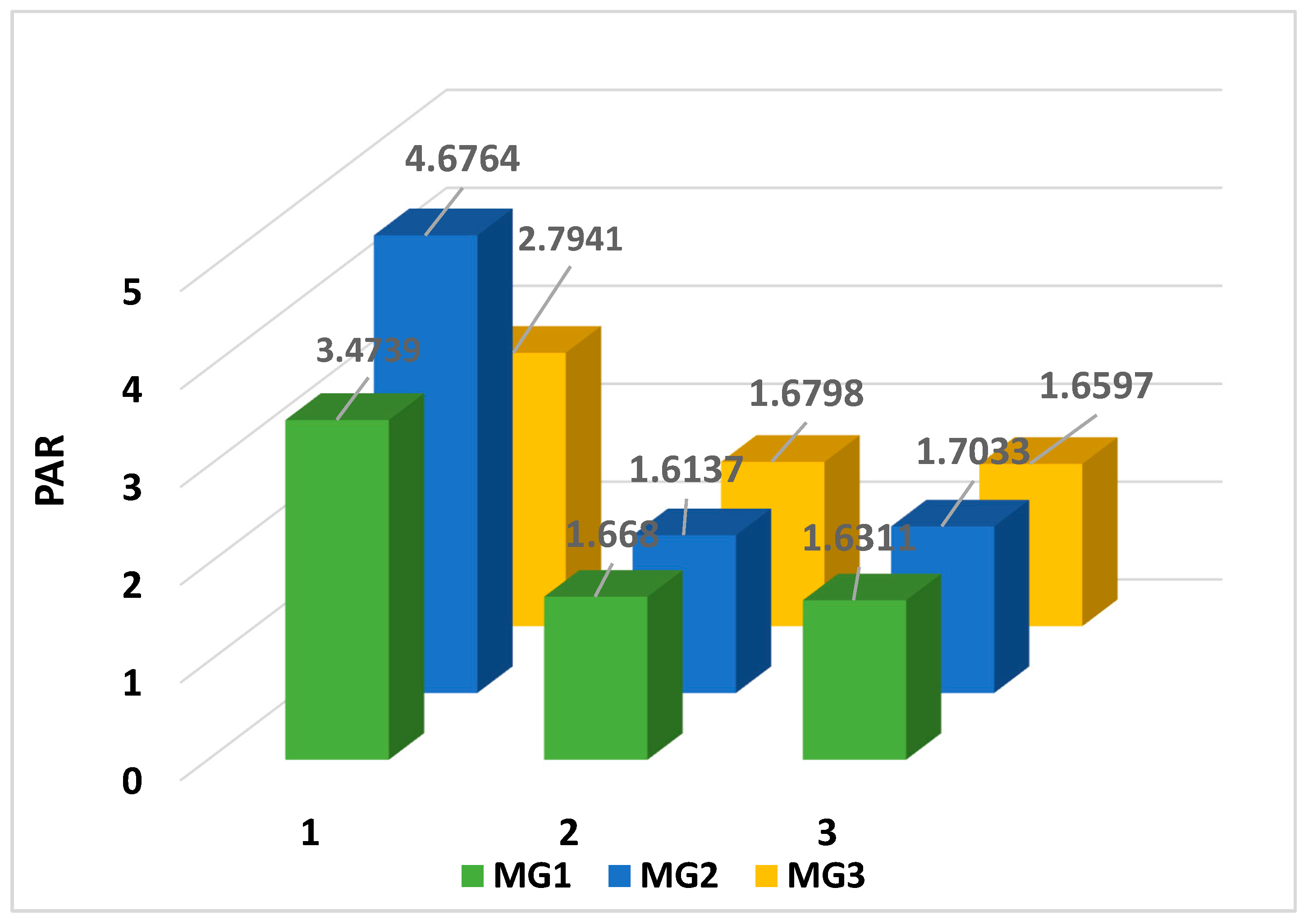
The increased amount of peak in MG2 is because of the reason that PV power is mostly available during the day, but the load slots defined by the prosumer routine is during the evening and morning periods where it is mostly relying on BESS energy and the power from LETM. The PAR for each scenario using the MJLBO algorithm is summarized in Figure 31.

5.6. User Disomfort

The user discomfort of each scenario is compared and is summarized in Figure 32. The minimum possible user discomfort occurs when all load appliances start operation at their corresponding defined starting time slots. In scenario 1, starting slots are randomly selected from the operation window and have the highest discomfort. Comparatively, in scenario 2, the user discomfort is minimum among all scenarios. The combined system discomfort in scenario 2 is obtained using MJLBO and the maximum discomfort in this scenario is for the JAYA algorithm. In scenario 3, with the MJLBO algorithm, the user discomfort is comparatively the same as scenario 2 as the algorithm optimizes the time slots corresponding to other objectives.

6. Conclusions

In this paper, a new energy management system is proposed for optimally scheduling the electricity load appliances in a multi-microgrid residential system. The system includes the use of local energy trading markets (LETM), 100% renewable energy resources (RER), and electric vehicle (EV) load for multi-objective purposes. Algorithms such as JAYA, TLBO, JLBO, and the proposed MJLBO are used to optimize the scheduling problem and validate the results. The scheduled microgrids trade electricity in the local power market to sell surplus electricity and buy electricity to cover corresponding demand from the LETM using a single-price market clearing price (MCP) mechanism. The proposed MJLBO algorithm reduces the net operation cost of each microgrid and improves the utilization of RERs while optimizing other objectives such as electricity cost, RES utilization, reduction in peak-to-average ratio (PAR), and user discomfort. The algorithm also reduces electricity costs by 12% and 10% for MG1 and MG2, respectively, and increases profit by 21% for MG3 as compared to the unscheduled system. Overall, the proposed system is generic and can be implemented for any number of microgrids and homes. Future work may include demand-side management with seasonal variation, sensitivity analysis, present worth, and cost analysis over a longer period of time.