
Dependence Analysis for the Energy Sector Based on Energy ETFs

1
Department of Financial Investments and Risk Management, Wroclaw University of Economics and Business, 53-345 Wrocław, Poland
2
Department of Econometrics and Statistics, Nicolaus Copernicus University in Torun, 87-100 Toruń, Poland
*
Author to whom correspondence should be addressed.
†
These authors contributed equally to this work.
Energies 2023, 16(3), 1329; https://doi.org/10.3390/en16031329
Submission received: 5 December 2022
/
Revised: 17 January 2023
/
Accepted: 23 January 2023
/
Published: 27 January 2023
(This article belongs to the Special Issue Energy Economics: Markets, Pricing and Policies)
Abstract
:This study investigates the effects of crude oil and natural gas future returns on energy stock portfolios. We consider returns of portfolios of energy companies approximated by energy ETFs and returns of Brent crude oil and natural gas contracts listed on the US market from January 2015 to September 2022. To study the relationship between Brent crude oil, natural gas, and ETFs, we apply Granger causality in mean and variance, Dynamic Conditional Correlation and the tail dependence-focused copula approach. The research hypothesis regarding the dependence between energy ETFs and the underlying energy risk factors—crude oil and natural gas, and therefore, the existence of hedging or diversification opportunities, was verified. Our empirical findings indicate that crude oil has a medium effect on energy ETFs, and for natural gas it is even lower in the analyzed period, so hedging opportunities are weak, but opportunities for diversification arise.
1. Introduction
The energy sector is strategic for every country, and it determines the development of every economy. As the global economy grows, energy production needs to be increased. Conventional sources such as coal, crude oil, and natural gas are expected to decline long term, and renewable sources are bound to increase.
Apart from its importance, the energy sector is not homogeneous. It consists of companies that use, process, or produce energy from nonrenewable or renewable sources. Natural resources such as crude oil and natural gas are fundamental macro variables for economic development (see the paper by Jones and Kaul [1]). Fluctuation of petroleum and natural gas prices affects the performance of the economy. An increase in crude oil and natural gas prices causes a temporary decrease in total production as investors defer economic activity due to the increase in prices. Additionally, these prices go up, they can push the prices of other commodities, goods, and services, which in turn causes inflation [2].
Recently, la Torre-Torres et al. [3] found that natural gas and crude oil have become popular choices among energy futures contracts, used to hedge commodity price risk. Similar trends are noticeable when such contracts are considered for investment and speculative purposes. This is due to their close links with economic activity and overall prices, as well as being an effective source of portfolio diversification. Therefore, crude oil and natural gas are considered diversifiers and hedging assets during calm economic periods, as well as safe assets during economic recessions and periods of high political uncertainty.
The relationship between stocks and crude oil is volatile, with the correlation between the returns of stocks and crude oil swinging between positive and negative values. There are periods when the prices of stocks and crude oil change in the same direction, sometimes in opposite directions. On average, however, this correlation is positive [4]. This means that the possibility of hedging portfolios of energy and non-energy stocks with crude oil and natural gas is also fluctuating. Thus, clarifying the relationship between energy portfolios (Exchange-Traded Funds, ETFs) and crude oil and gas prices can help investors make efficient investment decisions and construct hedging strategies.
The oil market analysis shows that supply and demand shocks occurred in the years 2014–2016. The 2014 supply shock was related to the increase in oil supply by OPEC countries following the intensification of oil production in the US. From 2014 and 2016, respectively, oil prices decreased by 70% in 18 months. Low oil prices drag the prices of other energy commodities down, mainly coal but natural gas also. The 2008 demand shock, on the other hand, was caused by the global crisis and reduced the oil demand. Both shocks had far-reaching, but not identical, consequences for oil prices. The same is true about the COVID-19 pandemic. Oil prices on the world markets are not only affected by the discussions by OPEC, the US, and Russia about the supply reduction (Saudi Arabia drastically reduced its prices), but also by the consequences of a worldwide pandemic. Low oil prices also affected other energy commodities, but the price decrease was not as big in the case of natural gas. In the years 2018–2019, the highest oil price increases were caused by the political situation in the Middle East. The US ripped up the nuclear agreement with Iran, reinstating sanctions related to the oil trade. Another important factor was the deepening crisis in Venezuela. In early 2017, OPEC agreed to stop oil production, as did Nigeria and Libya. In effect, the price of oil began to rise. In the case of the supply shock in 2022, the increases in oil prices were caused by the political situation related to the Ukrainian war—the restrictions imposed on Russia and actions aimed at limiting the increase in energy prices, including natural gas. Moreover, the US tightened monetary policy and the US dollar became very strong, increasing the cost of purchasing oil. Another factor affecting oil prices is the perspective of a global economic slowdown. Finally, one should also note the decision of the OPEC countries regarding limiting oil production. All these factors, combined with low inventory levels and continued demand for energy commodities, indicate that oil and gas prices will rise again.
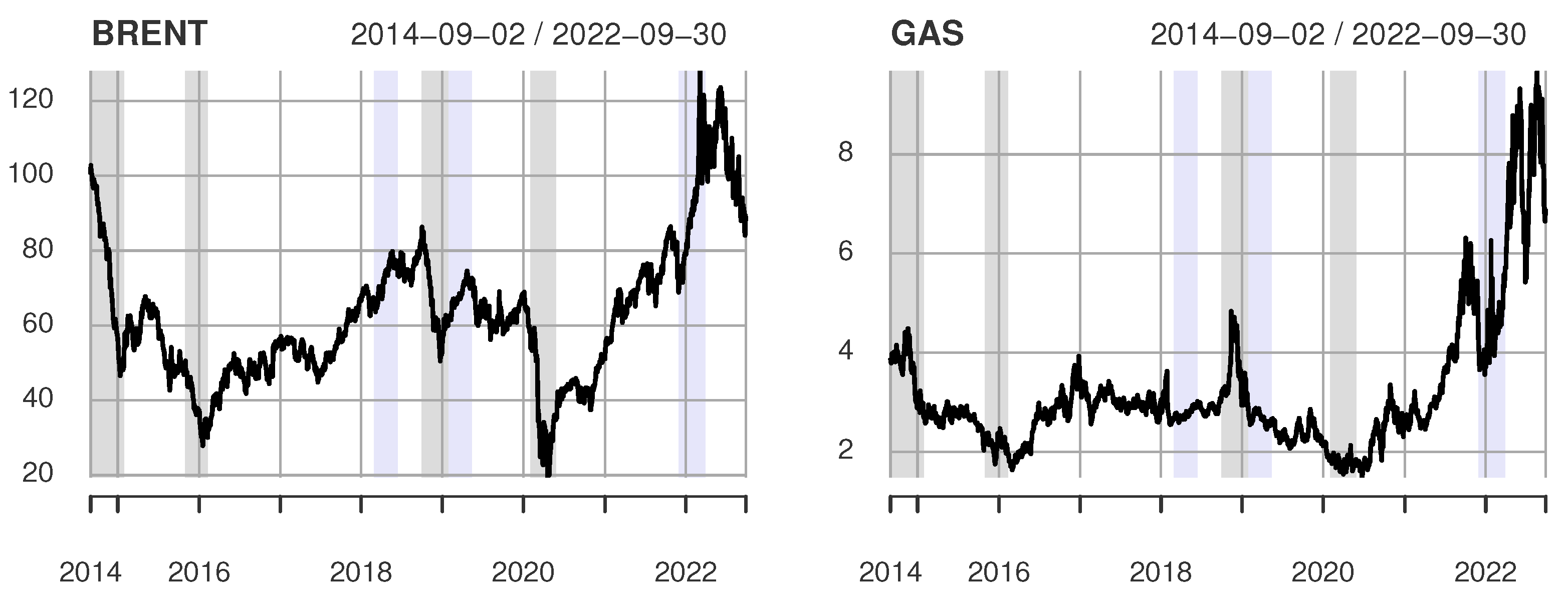
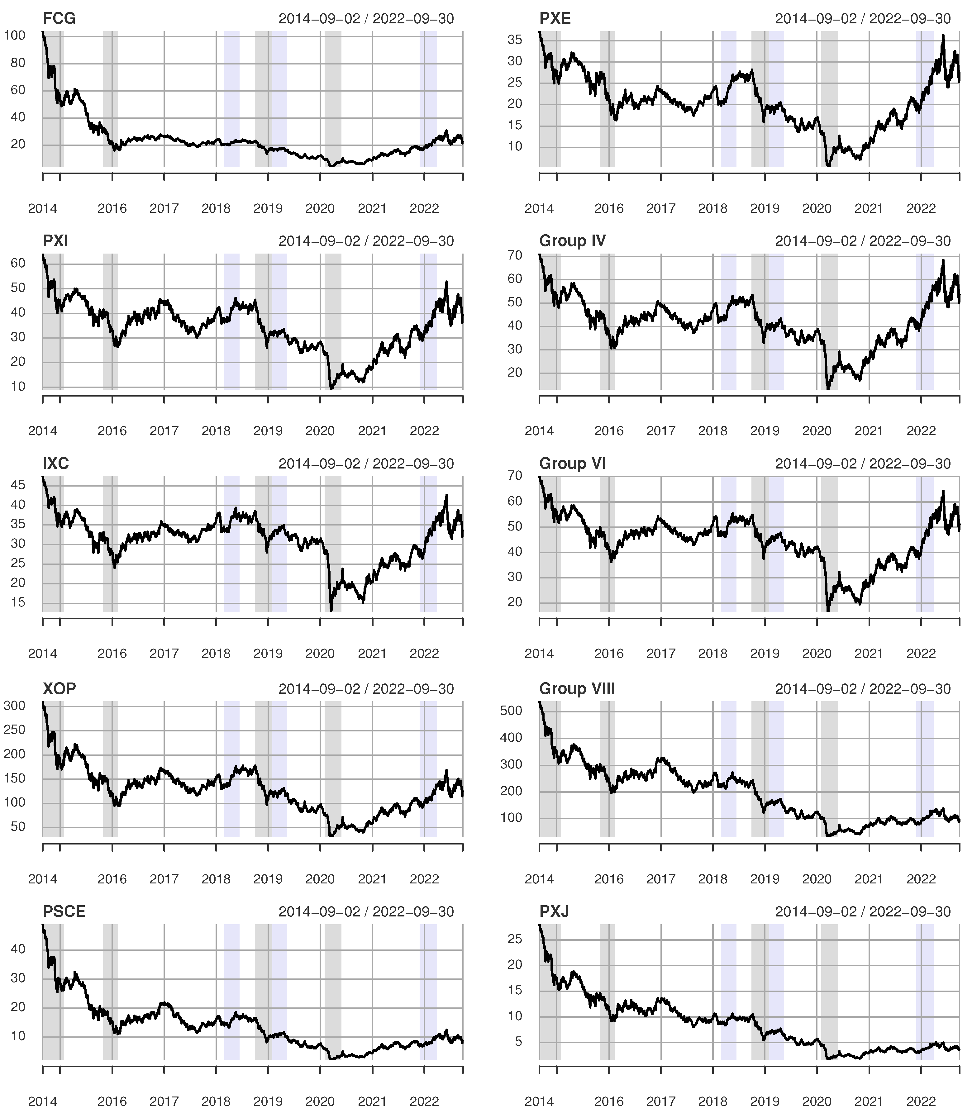
Therefore, in the study, we focus our attention on the following main periods of shocks (see Figure 1):
- Demand shocks: 2014–2016, 2020 (marked by the grey-shaded area);
- Supply shocks: 2018–2019, 2022 (market by the blue-shaded area).
During the periods of shocks in the oil market, oil and gas prices behaved similarly, except for the 2018–2019 shock.
Extreme events, e.g., the COVID-19 pandemic and the Russia–Ukraine conflict, influence the prices of crude oil and gas, and energy companies. In these periods, intensification of dependence is observed in the energy sector, therefore, it is challenging to look for benefits from hedging or portfolio diversification opportunities.
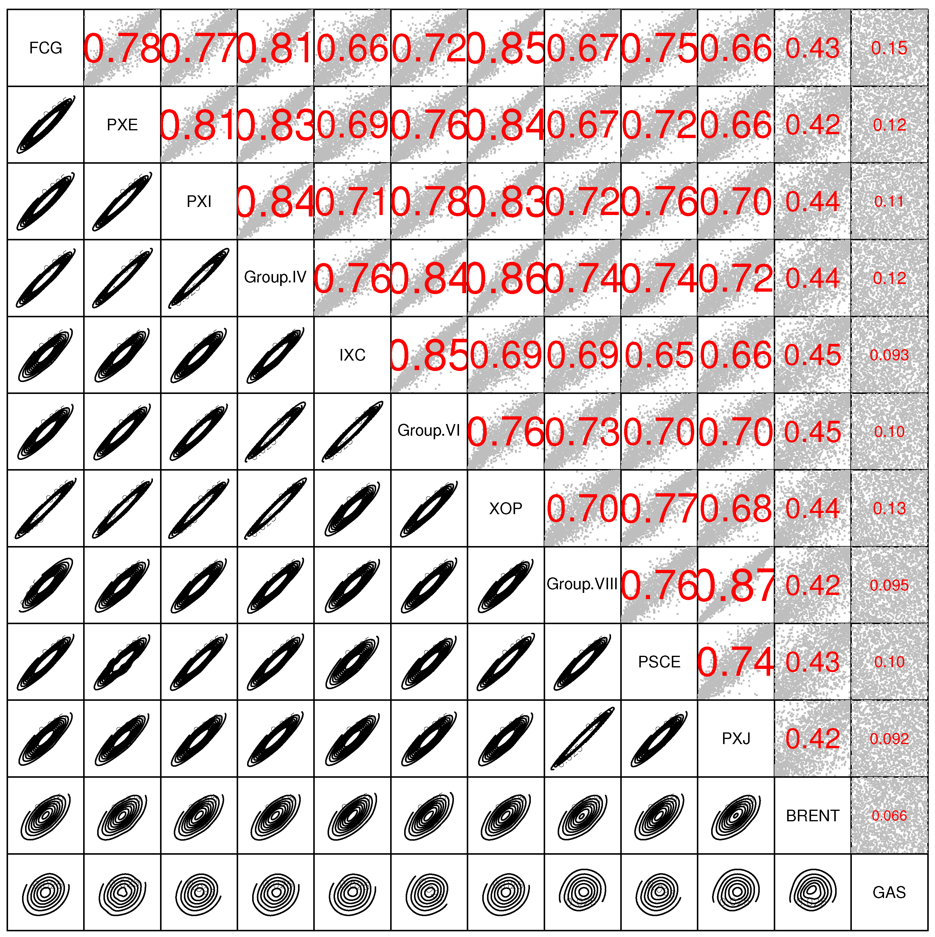
Analyzing the relationship between Brent crude oil, natural gas, and ETF returns (Figure A1) points to the possibility of using crude oil or natural gas as diversifiers of the energy portfolio. Based on this preliminary conclusion, the paper investigates the transmission of oil price changes and natural gas changes to energy portfolio returns. We examine the following research hypothesis: there is a dependence between energy ETFs and the underlying energy risk factors—Brent crude oil and natural gas; therefore, hedging or diversification opportunities exist.
To the best of our knowledge, this study is the first in the literature to gauge the relationship between Brent crude oil and natural gas price changes and energy portfolio returns using a large sample of 18 ETFs tracking energy companies (for approximately 9 years), finally clustered into 10 groups. Moreover, the study addresses the time-varying nature of the causal links between crude oil price shocks and ETF returns, as well as natural gas and ETF returns. Finally, it is a comprehensive insight into the energy market relationships and an assessment of hedging and diversification opportunities for energy portfolios, as in addition to causality analysis, we also apply DCC and copula-based approaches.
The organization of this paper is as follows. The next subsection reviews the literature. Section 2 describes the data, their characteristics and the methodology used in the study. The results of the empirical investigations are presented in Section 3. The next section explains the significance of results, while the last section concludes and discusses future research opportunities.
Literature Review
Since the groundbreaking study of Jones and Kaul [1] found that stock market returns respond negatively to changes in crude oil prices, many researchers have investigated the relationship between crude oil price shocks and the overall stock market. Most studies indicate a negative relationship between crude oil prices and stock returns, e.g., [5,6,7,8,9], however, some studies show that this relationship is positive, e.g., [10,11]. Nevertheless, other studies find that the crude oil price does not affect stock prices, e.g., [12,13,14] or that these effects are ambiguous, e.g., [15].
Many different methods were applied to the analysis of the dependence between crude oil and stock: Vector Error Correction Model, e.g., [5,15,16,17], ARDL Models, e.g., [18,19,20,21], Dynamic Conditional Correlation, e.g., [22,23,24], Granger causality analysis, e.g., [1,12,25,26,27,28], quantile regression, e.g., [29,30,31] and copula approach, e.g., [11,13,32,33]. These mentioned methods focus on the time domain aspect of the data.
Less research has focused on the impact of crude oil and natural gas prices on energy companies, e.g., [17,34], and in general, there is less research on natural gas [34] than on crude oil.
Ozdurak and Ulusoy [35] investigate the impact of energy-related ETFs on crude oil prices. They focus on price discovery of crude oil prices by applying causality tests. ETFs used in the study replicate commodity indices. Tang and Xu [36] examine nine leveraged ETFs related to crude oil—five are based on portfolios of oil stocks, and the other four use commodity futures to track the price of crude oil itself. The authors find that stock-based ETFs are much more correlated with the stock market than with crude oil prices, whereas the reverse is true of crude oil ETFs. Naeem et al. [37] explore the average and extreme dependence between ETFs (energy and commodity) and WTI crude oil prices by using EGARCH-copula models. The authors use static and time-varying copulas. Their results show strong positive correlations of energy and commodity ETFs with oil prices and that time-varying copulas outperform static copulas.
This study focuses on the energy sector on the stock exchange and the relationships between Brent crude oil, natural gas prices and energy portfolios. We use energy ETFs as proxies for energy stock portfolios. Energy ETFs selected for this study track energy indices consisted mostly of companies in the energy sector (92–100%). For natural resources, we use Brent crude oil and natural gas futures’ prices listed on the US market from January 2015 to September 2022.
Exchange-traded funds have existed on the US market since 1993 and in Europe since 1999. They track an index and are an alternative to an index mutual fund for risk-averse investors. Since they can be bought or sold at any time of the day, ETFs have and advantage over open-ended mutual funds. A classical index is a non-investment asset, and an ETF is. ETFs are characterized by high liquidity and allow investors to gain quick exposure to the underlying index. Perhaps for this reason, ETFs became a crucial tool for information dispersion. ETFs that track crude oil and gas or energy-related companies enable investors to invest or hedge in the energy sector and provide diversified portfolio strategies. Thus, ETF-hedging demand in the energy sector has been increasing due to the high volatility of energy prices [35].
Based on the literature review, to provide a more comprehensive and precise analysis of the overall dependence between energy portfolios and crude oil and gas, we decide to employ three methods: Granger causality (in mean and variance), Dynamic Conditional Correlation, and copulas with tail dependence. All of them focus on time domain aspects of data and, in that sense, are consistent. In this strand of literature, our study contributes by quantifying the time-varying causal relationship, copula, and DCC between Brent crude oil, natural gas, and energy ETFs, which is not considered in the existing literature related to the energy market. To the best of our knowledge, this is the first paper to apply the rolling Hong test to explore these relationships.
Many studies investigate the interdependencies of oil prices and stocks or stock indices, but there is a lack of such research for the energy sector on stock exchanges. Although the dependencies between the returns of companies in the energy sector, as well as the impact of such factors as crude oil and gas on them, are expected to be strong, the direction of this relationship seems unclear. Finally, we consider using energy ETFs to approximate a portfolio consisting of energy companies and futures on Brent crude oil and futures on natural gas to investigate the strength and direction of dependence, also in the tails of the distribution.
2. Data and Methods
2.1. Data
The data encompass daily closing prices of all energy ETFs listed on the US market between 1 September 2014 and 31 September 2022 and of Brent crude oil futures and natural gas futures prices. Table A1 shows the name of each ETF, its ticker, net assets value, energy sector weight, fund family, and the underlying index. The data source is Yahoo Finance (accessed on 1 October 2022) (https://www.yahoo.com).
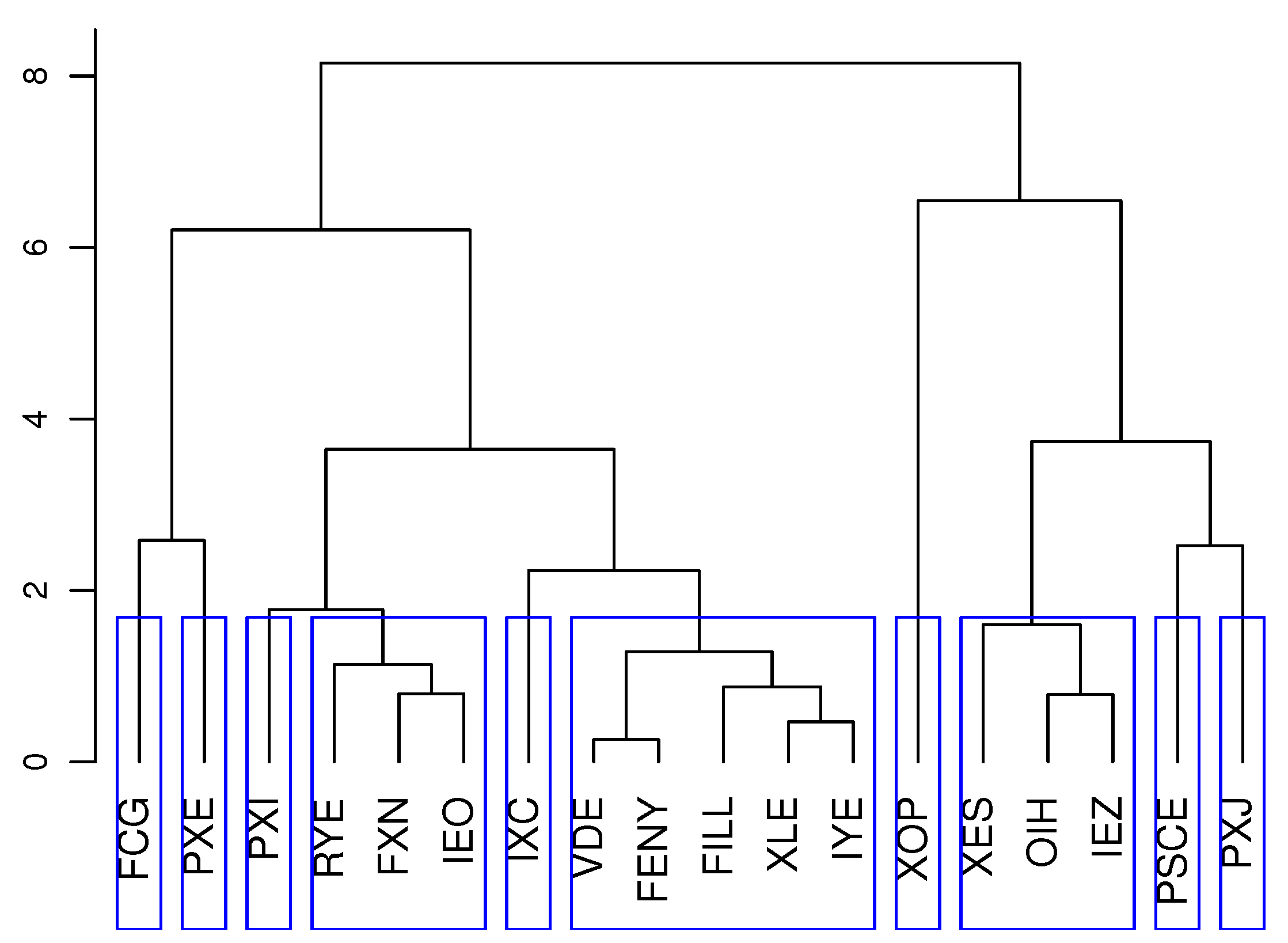
Initially, we analyzed the composition (based on the top ten holdings) of energy ETFs and their prices and returns individually, but as we observed some similarities between them, we decided to use clusters. In clustering the ETFs, we used two approaches: analysis of the ETFs’ holdings and the ETFs’ time series statistical parameters (mean, standard deviation, kurtosis, skewness, and correlation with Brent crude oil and natural gas). Finally, we created ten clusters, which were a compromise between ETFs’ holdings and time series characteristics. The clustering result obtained using Ward’s method is shown in Figure A2. The composition of the individual clusters is shown in Table A2, with most clusters being single-component. In the case of multi-component clusters, their rate of return was calculated as the rate of return for an equally weighted portfolio.
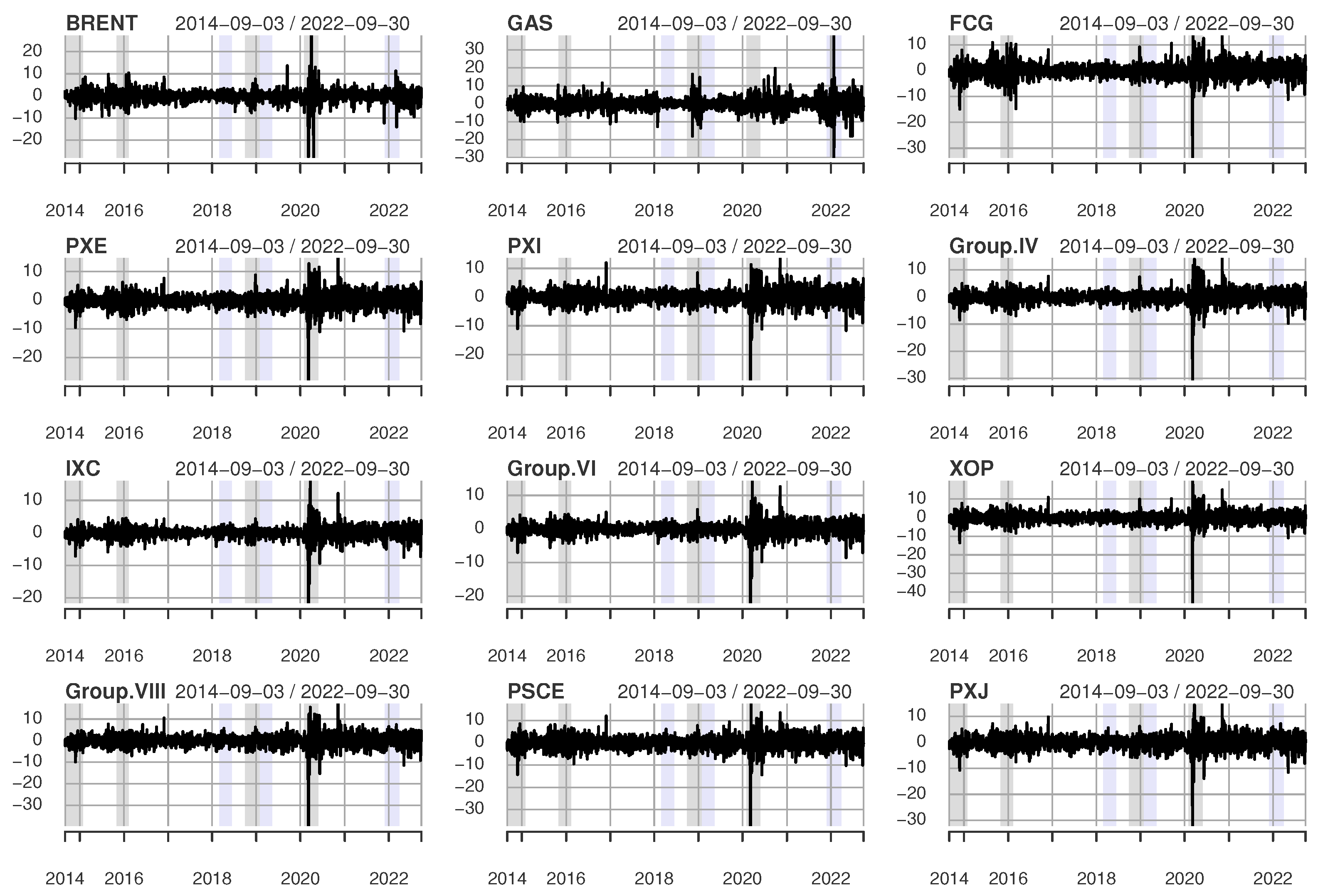
Prices of clusters of ETF, Brent crude oil, and natural gas over the analyzed period are presented in Figure 1 and Figure A3 display different behavior. According to the unit root tests—the Augmented Dickey–Fuller (ADF), Phillips–Perron (PP), and the Kwiatkowski, Phillips, Schmidt, and Shin (KPSS) tests (not reported here)—these prices are not stationary. Therefore, we analyze logarithmic percentage returns (see Figure A4).
Descriptive statistics for the rates of return and selected tests are presented in Table A3. The results show that the daily averages of all return series are negative, except for natural gas which has a positive average over the sample period. Brent crude oil has the lowest mean of daily returns over the period. In addition, the daily movements in natural gas prices exhibit the highest volatility. The volatility of crude oil is high but comparable with a few ETFs. The Jarque–Bera normality test rejects the normality of all the return series. In line with the literature-based expectations regarding the characteristics of stock returns, all ETFs, natural gas, and crude oil are leptokurtic and exhibit strong negative skewness (except for natural gas, whose skewness is positive). The Ljung–Box Q statistics show that the return and squared return series mostly do not exhibit serial correlations, and the returns are uncorrelated across time. Only in the case of natural gas was autocorrelation detected. Engle test results confirm the existence of the ARCH effect in all series. We employ unit root tests, namely, Dickey–Fuller (ADF), and the Kwiatkowski, Phillips, Schmidt, and Shin (KPSS), and find that all series are stationary, I(0).
2.2. Methodology
We chose a threefold approach to capture different aspects of dependencies at the time domain. First, we analyze the causal relationships in static and dynamic versions. The rolling causality test proposed by Lu et al. [39] has the following advantages over conventional causality methods: it reflects the dynamics of causal links, permitting the identification of the specific time periods during which significant Granger causality exists between time series; allows testing for causality in mean and variance from a dynamic perspective; makes it possible to detect unidirectional and bidirectional causality; allows to capture, e.g., asymmetry, fat tails, volatility clustering in financial time series, whose no consideration may lead to misleading results on Granger causality [38].
Next, we use correlations and their potential dynamics within conditional correlation models. According to Engle [40], the Dynamic Conditional Correlations GARCH model provides a very good approximation of a variety of time-varying correlation processes.
The third method applied in the study are copulas, used to estimate the tail dependence between assets. Modeling dependence using copulas is flexible in describing asymmetric dependence arising from the joint behavior of assets separated from their marginal behavior. Extreme events, fat tails of the distribution and bivariate asymptotic dependence are important aspects of risk hedging and diversification.
Based on the properties of the studied time series, we apply the following models from the ARMA-GARCH family: GARCH, EGARCH, IGARCH, GJR-GARCH, APGARCH, and AVGARCH. We use different distributions of the residuals, such as normal distribution, the Student’s t distribution, Generalized Error Distribution (GED), and their skewed versions. We selected the GARCH model employing the Akaike (AIC) and Bayesian (BIC) information criteria. Table A5 presents only the estimation results for the best-fitted models according to these criteria, including the minimum criteria values.
To capture the time dependence in rates of return, the univariate dynamics are described by ARMA(p,q) model in the following form [41,42]:
where , , —a closing price at time t, —the conditional variance modeled as a GARCH family process.
The autoregressive conditional heteroskedasticity (ARCH) models were introduced by Engle [43] and their generalization, the GARCH models by Bollerslev [44]. Let the model be a standard GARCH(q,p) model [44] of a form:
where —an intercept, —the residuals from the ARMA model.
When the conditional variance estimated by the GARCH(p, q) from Equation (2) process shows strong persistence, , an integrated GARCH (IGARCH) model is recommended. In the IGARCH model, the second moment does not exist, but the process shows a short memory.
The most important limitation of the GARCH model is that it cannot capture asymmetric performance well. Later, to improve this problem, EGARCH, GJR-GARCH, and APGARCH were proposed. The best-fitting models in our research are:
- The Exponential GARCH (EGARCH) model [45]:where the coefficient captures the sign effect and the size effect. is the expected value of the absolute standardized innovation ;
Models are estimated using the Quasi Maximum Likelihood method (QML).
2.2.1. Causality Relationship
Granger first introduced the concept of causality in 1969. Since then, many different methods for testing causality in Granger’s sense have emerged. In practice, vector autoregressive models (VAR) are most commonly used to study causality in the mean.
Let us consider two stationary time series: , . It is additionally assumed that , which are sets of time series information. Then, is the Granger cause of in mean with respect to [48]:
Whereas, is the Granger cause of in variance if [49]:
where is the conditional mean of .
Hong [50] proposed test statistics, which include Cheung and Ng test [49] and the Granger-type test [51] as special cases. He proposed one-sided asymptotically normal tests based on the cross-correlation function (CCF) of standardized residuals. Let us assume:
and is the cross-correlation of standardized residuals (, ) with lag j (; T—size of sample).
Then, Hong’s test statistics are as follows:
- Unidirectional Granger causality ():
- Bidirectional Granger causality ():
where is a weighting function and M is a positive integer. and are approximately the mean and variance of the generalized version of Cheung and Ng statistic [50]. Both and statistics have an asymptotic standard normal distribution . As it is a one-sided test, the upper-tailed critical values should be used [50].
As dynamic relationships between variables can change over time, a time-varying Granger-causality test is also used in the empirical literature. For this purpose, Lu et al. [39] propose a simple and intuitive approach of estimating Hong tests in rolling subsamples.
Let S denote the size of a subsample () and , are the standardized residuals of the stationary time series . Then, Hong’s rolling test statistics are as follows [39]:
- Unidirectional Granger causality ():
- Bidirectional Granger causality ():
- Instantaneous rolling Hong test for short ():
where is j-th lag of the cross-correlation coefficient between and in the subsample , is a weighting function, M is a positive integer and:
For all tests, if .
In rolling Hong tests, an appropriate rolling sample size S is crucial. If S is too small, the test will not yield valid results; if S is too large, there will be a long delay in detecting changes in Granger causality [39]. Lu et al. [39] determine a subsample size such that both the probability of making a Type I and Type II error are the same at 5%. The sample size we applied for the rolling Hong tests is of about 100.
The test procedure for the time-varying Hong test is similar to the static Hong test and it can be summarized as follows:
- Select the best-fit ARMA-GARCH model from the ARMA-GARCH class;
- Choose a rolling sample size S and compute the sample cross-correlations () of standardized residuals for each subsample;
- Choose an integer, M, and spectral window ;
- Compute the test statistics of Hong’s rolling tests.
This procedure leads to a total number of test statistics. If the test statistics at time t are bigger than the critical value at a given significance level; there is significant Granger causality at time t. We assumed a 5% significant level in this study, meaning the critical value equals 1.645.
Since the lagged dynamic correlations in financial markets usually tend to be zero for large lags, the Bartlett kernel is most commonly used in empirical studies [25,38,39,52]. M is a lag truncation value that induces a zero contribution for cross-correlations with a lag . In other words, only cross-correlations up to lag M contribute to causality evaluation. For this reason, we decided to use the Bartlett kernel and set for the rolling Hong test.
2.2.2. Dynamic Conditional Correlation
The dynamic conditional correlation model DCC-GARCH [40] is defined by the following equations:
where:
- —a diagonal matrix of time-varying standard deviations from univariate GARCH models;
- —a vector of the standardized residuals ;
- —a time-varying conditional correlation matrix of the ;
- –an unconditional correlation matrix of the ;
- —a diagonal matrix composed of the square roots of the diagonal elements of .
The model is estimated in two stages using the Quasi Maximum Likelihood (QML). In the first stage, we estimate the univariate GARCH models for each asset series [40,53,54]. In the second stage, we use the residuals estimated during the first stage, transformed by their standard deviation to estimate the parameters of the dynamic correlation.
We apply the multivariate Student’s t distribution as the null hypothesis of a multivariate normal distribution is rejected. The estimated DCC-GARCH models satisfy the constraints imposed on conditional variance and conditional correlation for pairs of returns.
2.2.3. Copulas
The asymptotic dependence of random variables in tails solely depends on the copula [55]. This approach allows investigating the dependence in variance and in tails, which provides absolute control of the marginal latent trait distributions and accommodates several dependence structures. Such an approach would be impossible using standard dependence measures. The concept of the copula was first introduced by Sklar [56]. Sklar’s theorem provides the theoretical background for copulas. Following the theorem, there exists a copula C such that:
where F is two-dimensional joint distribution with the marginal distributions , of random variables .
If , are continuous, the copula C is unique:
where , for .
The proof is provided by, e.g., Nelsen [57].
Many families of parametric copulas (e.g., Gaussian, Archimedean) can be used to capture different dependence structures. This paper uses the following copulas: Gaussian, Student’s t, Frank, and Joe–Frank. The Gaussian, Frank, and Joe–Frank copulas are tail-symmetric and do not capture tail dependence. Student’s t copula has a symmetric tail dependence in both the lower and upper tails.
- Gaussian/Normal (N) copula:where N is the normal joint distribution and is the quantile of the univariate normal distribution;
- Student’s t/t (t) copula:where , is the joint Student’s t distribution and is the univariate Student’s t distribution with degrees of freedom;
- Frank copula:where ;
- Joe–Frank (BB8) copula:where , .
Survival copula is the copula of and instead of and , respectively. It couples the joint survival function to its univariate margins as a copula connects the joint distribution function to its margins [57]. Our focus is on extreme downside market risk, so we have examined the lower tail dependence in detail.
The tail dependence coefficients [55] are:
- Lower tail dependence coefficient:
- Upper tail dependence:
in case the limit exists, and (), dependence is present.
Instead of Pearson’s correlation coefficient in the copula theory, we use Kendall’s coefficient [55,57]. In this paper, we use functions from the VineCopula library in R [59].
We use the Maximum Likelihood Estimation (MLE) method to fit the copulas from the catalog of the pair-copula family (39 copulas considered). Then, to select the best-fitted copula, we apply the AIC. To measure the discrepancy between the hypothesized and the empirical model, we use the Goodness-of-Fit (GoF) statistics based on Kendall’s process proposed by Wang and Wells [60]. We also employ the parametric bootstrap described by Genest for the computation of p-values.
3. Results
In order to conduct the dependency analysis, the time series must be covariance stationary, so unit root tests of the returns are necessary. Table A4 shows the results of these tests. All returns are integrated of order 0, which means that they are stationary. Then, the best-fitting ARMA-GARCH model is selected.
Among GARCH family models, for most ETF returns, the EGARCH model with Student’s t innovation distribution fits best. For one ETF and Brent crude oil, the AVGARCH model with Student’s t and skewed Student’s t innovation distributions are selected, respectively. One ETF cluster is modeled using ARMA-AVGARCH with skewed Student’s t innovation distribution. For natural gas, the IGARCH model with Student’s t innovation distribution is used. All choices are made using the BIC criterion (see Table A5).
3.1. Causality Relationship
Volatility can be transmitted between Brent crude oil prices and stock returns even when the returns of the two markets are uncorrelated or do not exhibit causality in the mean. Causality in variance has become more important because of the increasing market integration due to economic and financial globalization and technological innovations in financial markets [38].
The essence of causality testing is to know the direction of the interrelationships between assets and the time required to react to anticipate changes. We apply Granger-causality tests (both: static and dynamic) in mean and variance to detect the Granger-causal relationships between crude oil, natural gas, and energy ETFs. Since we assume that crude oil and natural gas are the sources of increase or decrease of profitability of energy companies, the analysis is focused on one direction of the relationship (from crude oil/natural gas to energy ETFs). The relationship between selected 10 clusters of ETF and crude oil and 10 clusters of ETF and natural gas creates 20 pairs for analysis. For causality evaluation, we set the lag truncation value as , , and for static tests, and for the rolling Hong tests (for both: in-mean and in-variance tests).
Granger-causality in-mean tests (Table 1) indicate a causal link from Brent crude oil to all analyzed ETFs’ clusters (for all lags).
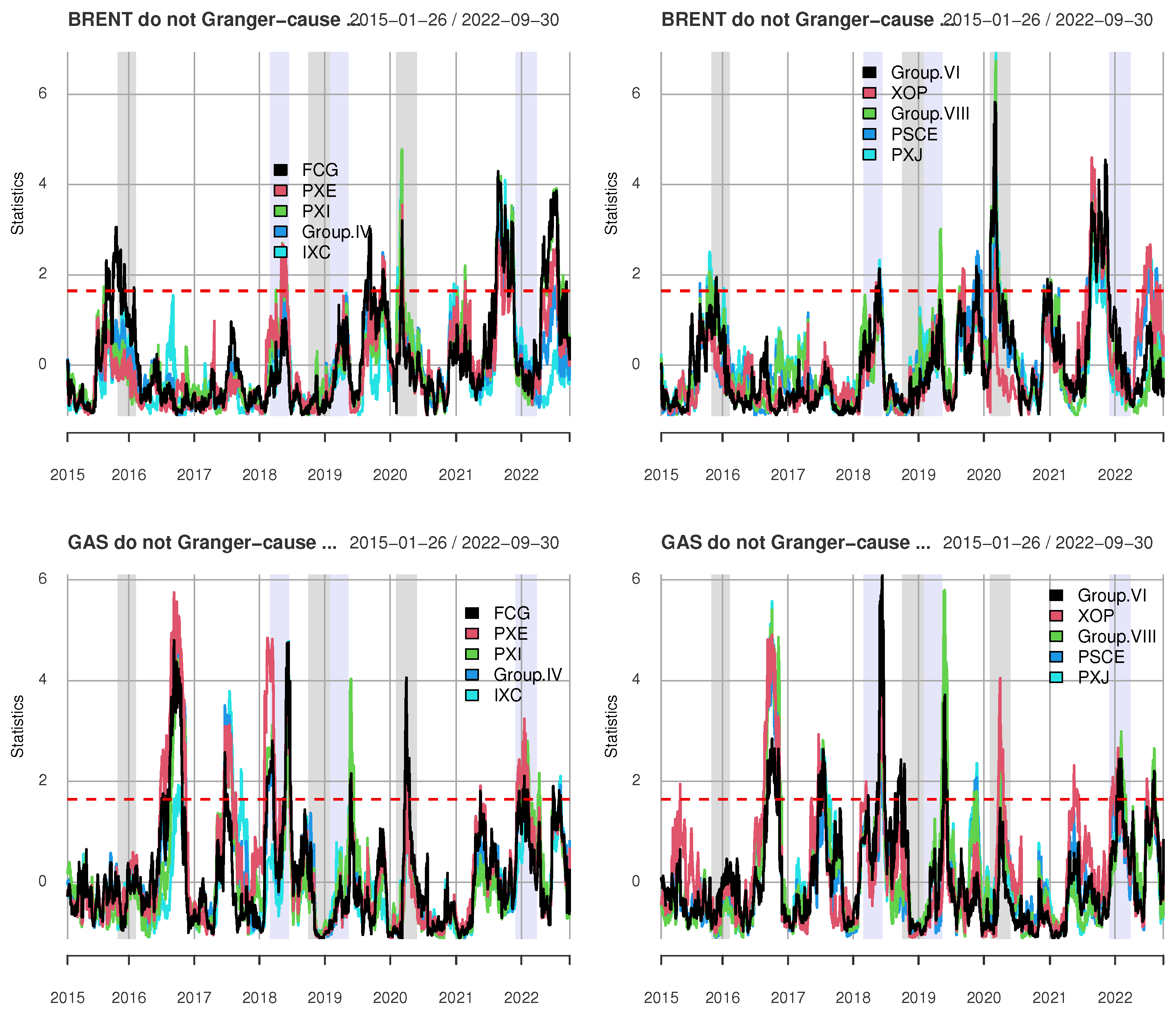
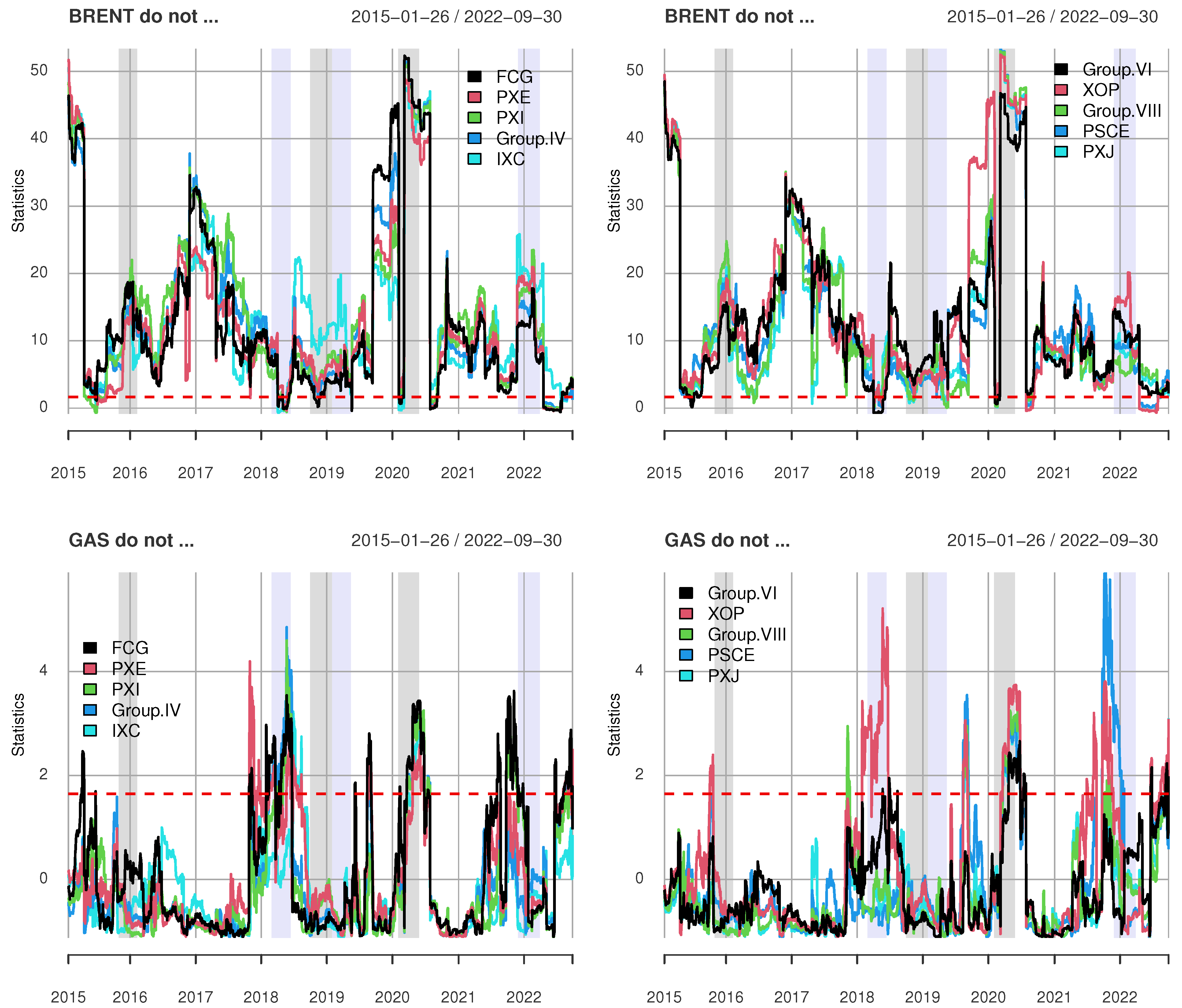
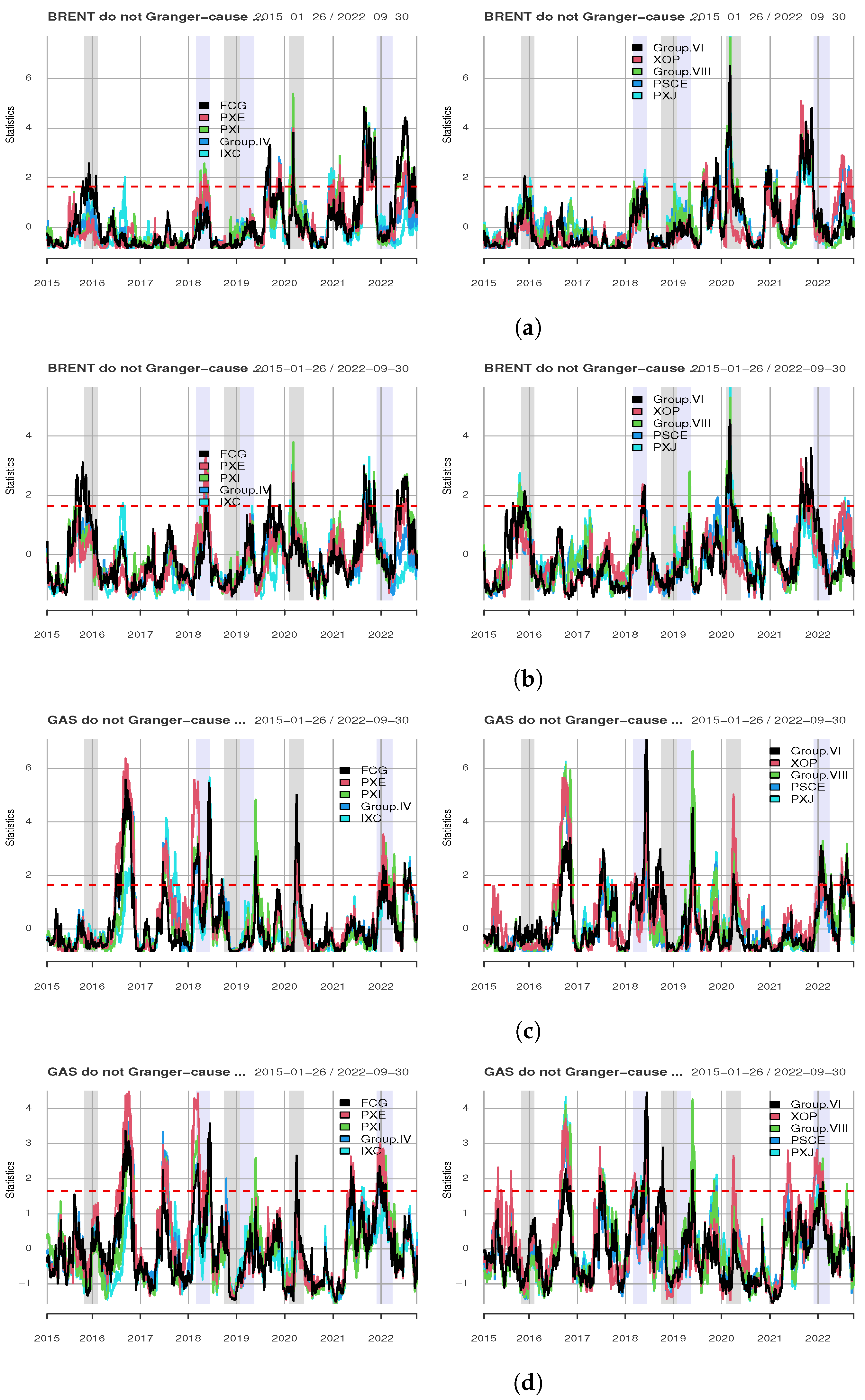
There is no causal link from natural gas to energy ETF’ clusters, but surprisingly, from energy ETFs to natural gas, it exists in 90% of cases (see Table 1). As these relationships can change over time, a time-varying Granger-causality test is also applied. The results of rolling test statistics for a unidirectional link from crude oil and natural gas to ETFs are shown in Figure 2, and for the instantaneous link—in Figure 3. The unidirectional Brent → ETF reveals that there are four main (for most ETFs, looking individually at each ETF, there are more) statistically significant causality episodes from crude oil to ETF. The first episode was in 2016, and the second was in 2020 (both were demand shocks) when crude oil prices decreased. The next episode occurred in 2021 before a supply shock, when crude oil prices increased, and the last in 2022—after a supply shock. The unidirectional Gas → ETF exhibits seven short-lived statistically significant causality episodes from natural gas to ETFs. Looking individually at each ETF, there are even more. The first episode was in 2016 after a demand shock, when natural gas prices decreased. The second episode was in 2017, and the next was in 2018 (supply shock), when natural gas prices increased. The fourth episode was in 2019 after the supply shock, and the next was a demand shock in 2020, when natural gas prices decreased. The sixth episode was a supply shock in 2022, when prices of natural gas decreased. The final, seventh episode occurred afterward, during a fast natural gas price increase.
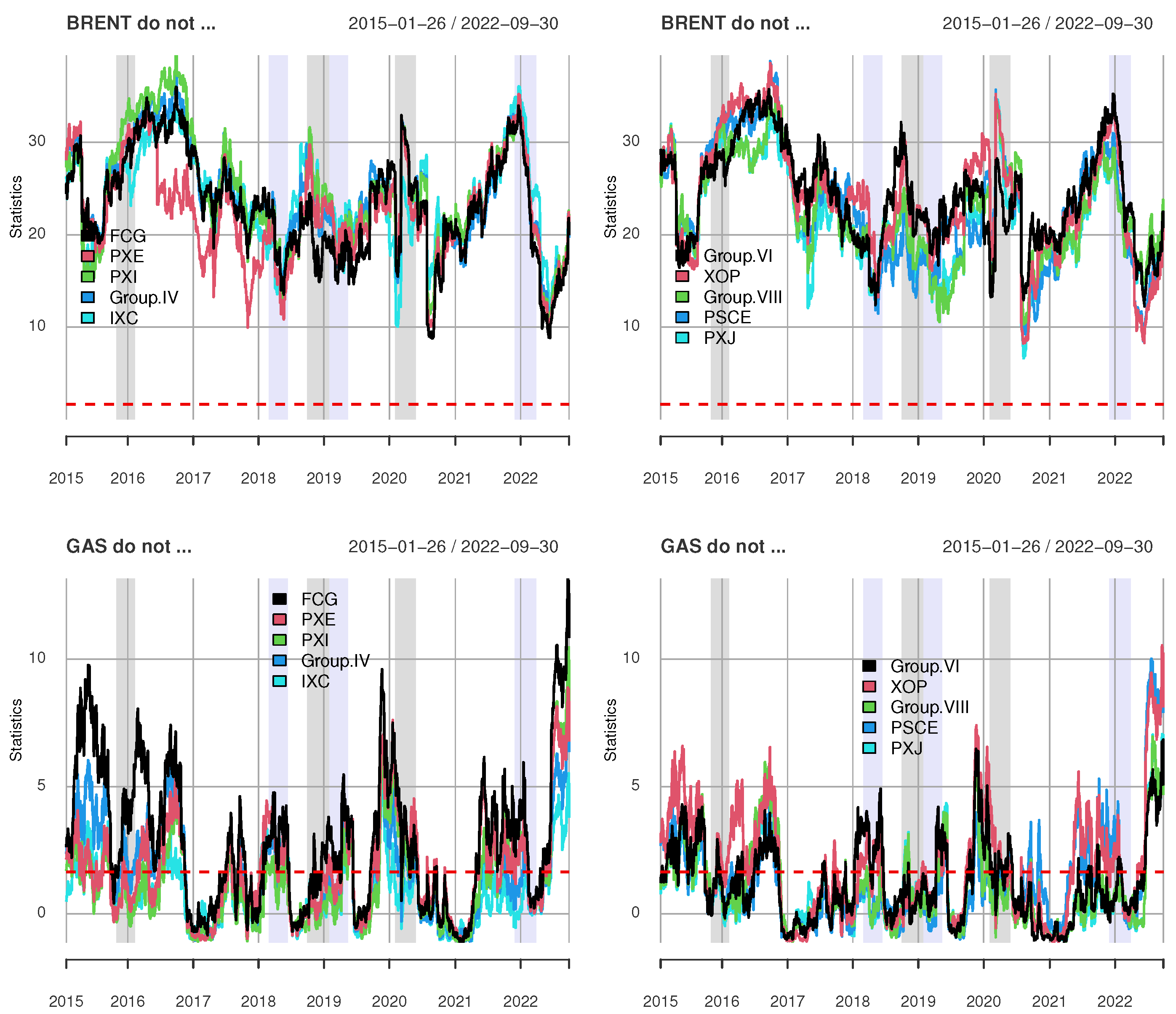
The instantaneous Granger-cause-in-mean from Brent ⇒ ETF experienced an all-time record. In the case of natural gas, there are many episodes of statistically significant causality (see Figure 3).
While the Granger-causality-in-mean tests indicate a causal link from Brent crude oil prices to energy portfolios returns, the Granger-causality-in-variance tests suggest a causal link from global crude oil market prices to energy portfolios returns in 70% of pairs (for ). In the case of natural gas, these tests do not detect causality in the variance (see Table 2).
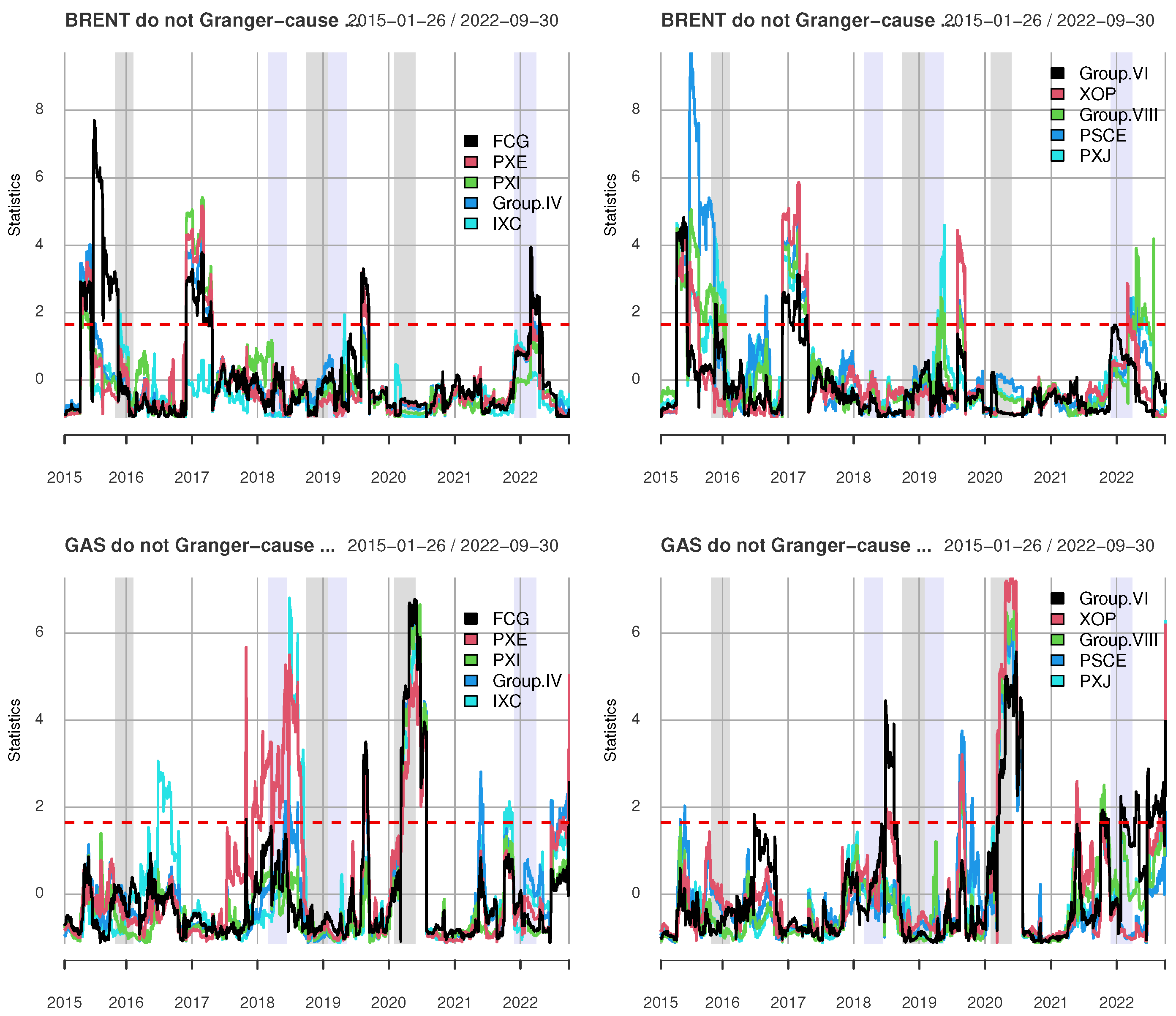
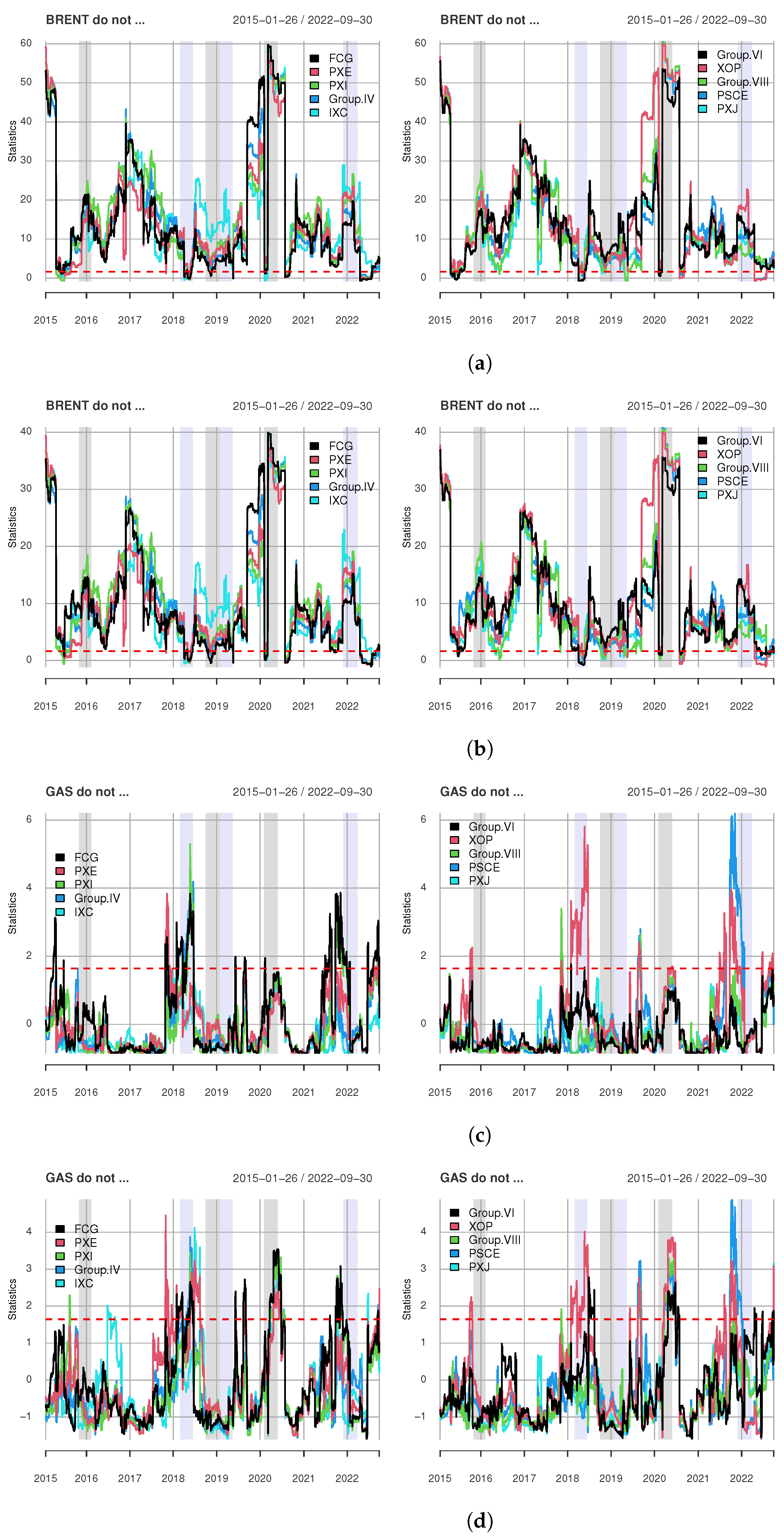
Time-varying Granger-causality tests in variance are presented in Figure 4 and Figure 5. The unidirectional Brent → ETF reveals four statistically significant causality in-variance episodes from crude oil to ETF. Similarly as before, for individual ETFs–there are more. The first episode was in 2015; the second was in 2017, when crude oil prices increased. The next episode is observed after shocks in 2019, when crude oil prices decreased, and the last one in 2022, after a supply shock, when crude oil prices increased. The unidirectional Gas ⇒ ETF exhibits three main statistically significant causality in-variance episodes from gas to ETF (more for individual ETF). The first episode was in 2018, when natural gas prices increased. The next episode was in 2020 (during a demand shock), and the last was in 2022, when natural gas prices increased.
The instantaneous Granger-cause in-variance (see Figure 4) from Brent ⇒ ETF experienced an all-time record. The instantaneous Gas ⇒ ETF exhibits four main statistically significant causality in-variance episodes from natural gas to ETF. Again, for individual ETF there are more. The first episode was in 2018, when natural gas prices increased. The second episode was a supply shock observed in 2020, when natural gas prices decreased. The next one was in 2021, and the last was in 2022, when natural gas prices increased.
We checked robustness by calculating rolling Hong tests for and . Figure A5 presents the values of unidirectional causality-in-mean tests, while Figure A6 shows the values of instantaneous causality-in-variance tests. The larger the value of M, the smaller the statistic. However, the main conclusion persists. The results also confirm it, for instantaneous causality-in-mean tests and unidirectional causality-in-variance tests not reported here.
3.2. Conditional Correlation
In the first stage, we estimate the univariate GARCH models. The particular specifications for each series and results of the tests conducted on the residuals in Table A5 in the Appendix are presented. In the second stage, the multivariate dynamic conditional correlation (DCC) models for pairs of crude oil and energy portfolios are estimated. The DCC parameters (, , and shape), collected in Table A6, for all pairs, sum up to a value close to 1. It indicates that the dynamic conditional correlations follow the mean-reversion process.
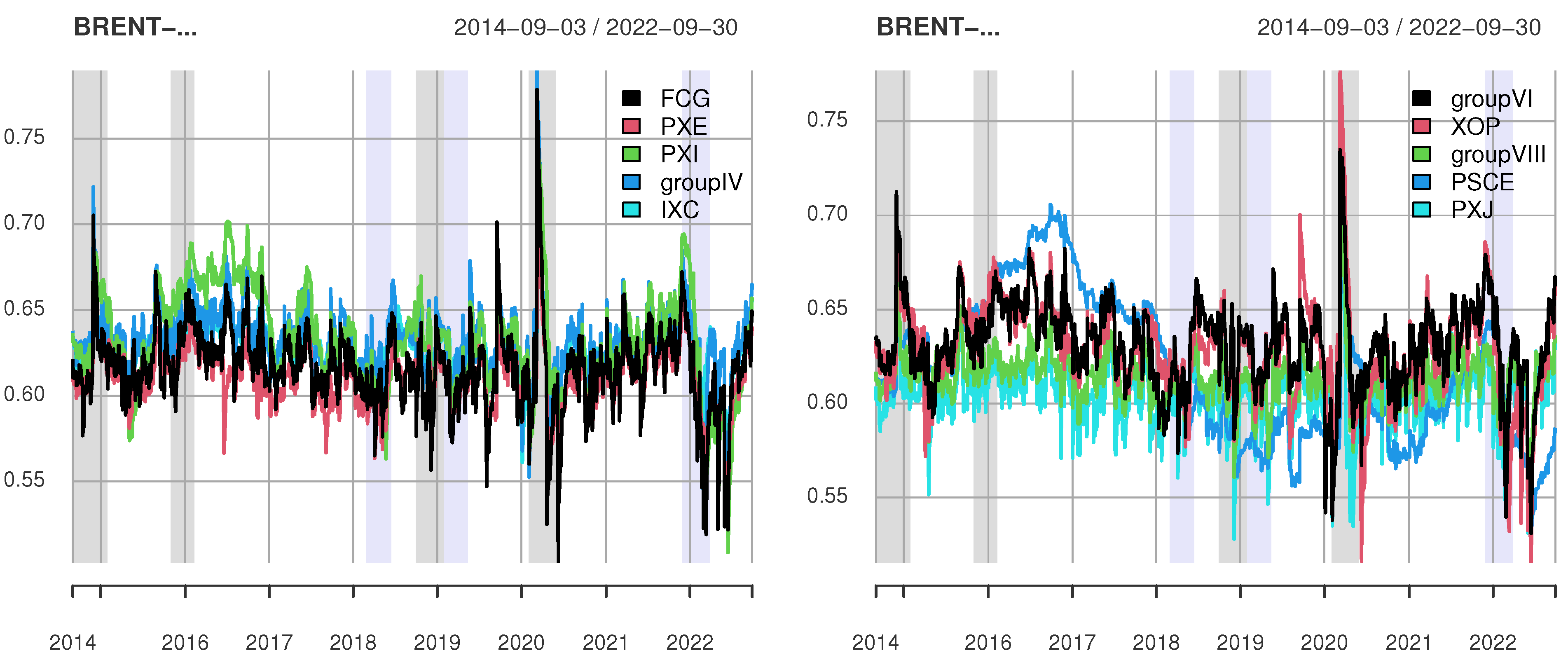
We apply the Engle and Sheppard test [53] for dynamic correlation to check whether the correlation is constant. The results in Table 3 indicate the constant correlation between natural gas and energy portfolios over the sample period, but the correlation between crude oil and energy portfolios depends on a particular ETF. For some ETFs, there are cases with constant correlation, and for others—with a non-constant one.
An illustration for Brent crude oil and ETFs is presented in Figure 6. It seems that for significantly non-constant correlation cases of supply shocks, the correlation decreases, and in demand shocks, it increases compared to the rest of the considered period, but this requires further investigation.
3.3. Copulas
The results of the dependence measures for Brent crude oil returns and energy portfolios are reported in Table 4 and Figure A7. The association measure, Kendall’s tau, is statistically significant and positive. Using Akaike and BIC criteria, Student’s t copula was found to be the best copula. The tail dependencies for this copula are very low, indicating nearly an independence between crude oil and energy portfolios.
The results of the dependence measures for natural gas and energy portfolios are reported in Table 5 and Figure A7. The association measure—Kendall’s tau—is statistically significant, positive, and very low compared with the association between crude oil and energy portfolios. Using Akaike and BIC criteria, the Gaussian copula was found to be the best-fitted one (in 70% of cases). Frank’s and Survival Joe–Frank copulas were also fitted. The tail dependencies for Gaussian copula, as well as Frank’s and Survival Joe–Frank, indicate independence between natural gas and energy portfolios.
4. Discussion
In general, the prices of energy, natural gas, and crude oil (in particular) are very volatile. In crude oil returns analysis, asymmetric GARCH models are often the most accurate. Salisu and Fasanya [61] investigate asymmetry in crude oil price shocks and volatility (WTI and Brent). They apply the Exponential GARCH (EGRCH) model and indicate that positive shocks affect volatility differently than negative shocks [61]. Our results regarding crude oil are consistent with Salisu and Fasanya [61], Echaust and Just [62], and Naeem et al. [37].
With respect to to natural gas in the study, IGARCH was fitted, but in the literature, different GARCH-type models were considered (e.g., TGARCH [63], Regime Switching [64]). For crude oil and natural gas modeling, two-state Markov Regime Switching models, e.g., [64,65,66,67] or stochastic volatility models, e.g., [68] were also applied.
The causal relationship between crude oil and ETFs and natural gas and ETFs was also investigated in order to obtain a complete insight into the dependence structure, i.e., to determine the cause of individual behavior. The presence of significant bidirectional causal relationships in the mean and variance between crude oil price changes and stock returns over all time horizons was found by Jammazi et al. It is consistent with the idea that crude oil and stock markets are tightly integrated and influence each other in the short, medium, and long term [38]. Similarly, in this paper, unidirectional causality in mean from crude oil price changes to ETF returns is confirmed, as well as the dynamic and instantaneous one. In-variance tests suggest a causal link from global crude oil market prices to energy portfolio returns in 70% of pairs. The case of natural gas is different. There is no causal in-mean link from natural gas price changes to ETF returns, but the dynamic tests indicate many short episodes of significant links. The same result refers to the in-variance test. Both Jammazi et al. [38] and this paper use time-varying causality tests proposed by Lu et al. [39] that are based on the causality procedures developed by Cheung and Ng [49], and Hong [50]. These tests are not popular in causality analysis for energy price changes and stock returns.
The copula approach investigates the dependence structure between crude oil/natural gas and stock returns. In our study for Brent crude oil and ETFs, the best-fitting copula is Student’s t. This is in line with the study by Avdulaj and Barunik [69], but in Aloui et al. [11], the asymmetric Survival Gumbel copula fits best. Best-fitting copulas for dependence between natural gas and ETFs are Gaussian, Frank, and the survival Joe–Frank copula. To examine the possible evolution of the dependence over time, the time-varying copula approach should be used as by Avdulaj and Barunik [69], Aloui et al. [11], and Naeem et al. [37]. Comparing the same three ETFs as the ones used in our study and WTI crude oil, Naeem et al. [37] found that time-varying SJC copula is the best-fitted model for pairs VDE-WTI, XLE-WTI and XOP-WTI. They have also identified normal time-varying copula for the pairs ICLN-WTI and PBW-WTI.
Our results are consistent with Naeem et al. [37], showing that energy ETFs offered enough strong, positive correlations with crude oil to be used as a tool for managing crude oil price risk.
Among the potential reasons for the limited benefits of diversification with commodities is the fact that the correlation between commodities and conventional assets increases significantly during unfavorable periods. This phenomenon is known as ’correlation clustering’ and means that correlations are not always negative or close to zero and tend to increase during periods of poor financial market performance [3]. Our analysis of crude oil using DCC confirms this fact, e.g., [3,70], but for natural gas, it does not. Our results show that dependence between crude oil and ETFs changes over time, and the correlation goes from zero to relatively strong and positive. In contrast, the dependency parameter between natural gas and ETFs is constant over time and remains close to zero. This is in line with the results by Delatte and Lopez [70].
Not much research has been focused on the impact of crude oil and natural gas prices on energy companies, and in general, there is even less research related to natural gas than crude oil in this area. Thus, this study could be extended in several ways. The time period, currency of assets (USD), and exchange for ETFs (NYSE, Nasdaq) limited the set of ETFs considered in the paper. Other energy type ETFs such as clean energy are excluded from the study. In further research, the set of ETFs could be extended. Further research could also be extended by considering fundamentals of oil market, taking into account driving forces for crude oil and natural gas, e.g., [71,72,73].
The calculations could be repeated for other energy price series and for other stock portfolios. The robustness of the causality results could be tested against causal measures other than those applied here. The dependence structure could be investigated by the time-varying copula approach. In the paper, any quantile type approach was not considered. Research could be extended by the use of cross-quantilogram to detect directional predictability from crude oil/natural gas to energy stock returns (as proposed by Han et al. [74]).
In our study, we focus on measuring dependency, further research could explore volatility transmission among energy ETFs, crude oil, and natural gas (e.g., network models, spillover effects, e.g., [33,75,76,77]) and wavelet methods to quantify the strength of oil–stock association at different time scales e.g., [38,78,79].
5. Conclusions
This paper contributes to the existing literature focusing on the impact of energy ETFs on crude oil and natural gas returns. First, we examined the return discovery and causality relationship between Brent crude oil futures and clusters of ETFs’ returns, natural gas futures, and clusters of ETFs. Existing studies focused on the relationship between equity markets and crude oil markets, whist natural gas has been less analyzed. However, ETFs are now an important source of information dissemination. To our knowledge, we find the only study of Ozdurak and Ulusoy 2020 [35] used energy ETFs and future prices investigating described dependence, and we have therefore decided to fill this gap.
We verified the causal relationships between crude oil and energy portfolios using static and time-varying causality-in-mean and causality-in-variance methods using Hong [50] and rolling Hong [39] tests, respectively. The results show that if one uses a causality test without taking the possible time-varying nature of the causal relationships, the causal link in-mean from crude oil to energy portfolio exists, but there is no link from natural gas to energy portfolios. Instantaneous causality from crude oil and natural gas to energy portfolios exists.
The unidirectional Brent → ETF in-mean analysis (both static and dynamic) suggests that crude oil and ETFs are linked. The evidence regarding the causality in variance demonstrates the transmission of information between crude oil and ETFs for most pairs (70% in the case of static test) and many significant link episodes (confirmed by the dynamic test). In the case of natural gas, static in-mean analysis indicates no links, but dynamic analysis confirms the existence of significant link episodes. Similarly, for in-variance analysis, the static approach does not detect any links, but the dynamic one shows significant link episodes. The main empirical finding is the presence of a significant unidirectional causal link in mean and variance between crude oil price changes and ETFs, and no causal link in the case of gas, except for many significant link episodes confirmed by dynamic tests in mean and variance.
There are cases with constant and non-constant correlations for crude oil and ETFs. It seems that for significantly non-constant correlation cases in supply shocks, the correlation decreases, and in the demand shocks, it increases compared to the rest of the period. However, it requires further investigation. In the case of natural gas, there is a constant correlation detected.
The characteristics of the time series indicated the need to apply the dependence analysis copula approach. Among different types of estimated copulas, the Student’s t copula fits best. The results of dependence measures such as Kendall’s tau and the tail dependencies are quite small for all the cases (very small for natural gas and energy portfolios). Moreover, the relationships are symmetric. This implies that crude oil and energy portfolios will have a similar relationship regardless of the state of the economy. The tail dependencies are weak for crude oil and zero for natural gas indicating independence between natural gas and energy portfolios. It means that for natural gas, diversification opportunities are greater compared to Brent crude oil.
The research hypothesis regarding a strong dependence between energy ETFs and the underlying energy risk factors—crude oil and natural gas—was rejected. The hedging opportunities are weak, but opportunities for diversification arise.
Our study has important implications for various traders, investors, and portfolio managers who want to reduce portfolio risk through diversification or to hedge against market risk (i.e., risk of crude oil price and natural gas). A better understanding of dependency is essential for minimum risk portfolio construction by using diversification or hedge against market risk using futures on crude oil or natural gas. Additionally, policymakers should not ignore the dependencies between crude oil and natural gas and the energy portfolios when trying to avoid the risk of contagion (causing high inflation), especially during extreme events and crisis periods.
Author Contributions
Conceptualization, K.K. and J.G.; methodology, K.K. and J.G.; software, J.G.; formal analysis, K.K. and J.G.; investigation, K.K. and J.G.; resources, K.K.; data curation, J.G.; writing—original draft preparation, K.K. and J.G.; writing—review and editing, K.K. and J.G.; visualization, K.K. and J.G.; supervision, K.K.; funding acquisition, K.K. All authors have read and agreed to the published version of the manuscript.
Funding
This research was funded by Wroclaw University of Economics and Business.
Data Availability Statement
This data can be found here: https://www.yahoo.com (accessed on 1 October 2022).
Conflicts of Interest
The authors declare no conflict of interest.
Appendix A
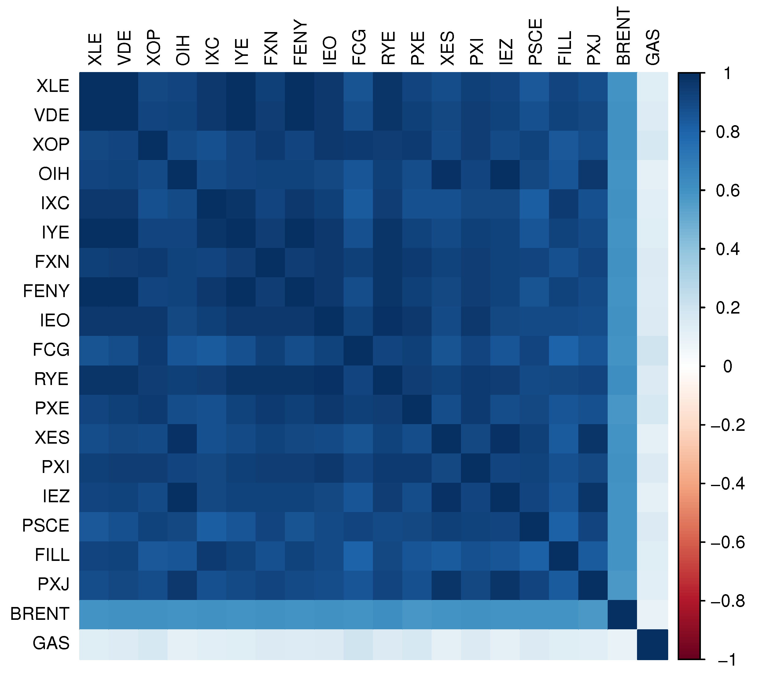
Figure A1.
Pearson correlation for returns of oil, gas, and ETFs.

Figure A2.
ETFs clustered by Ward’s Method with Euclidean distance.

Figure A3.
Prices of oil, gas and ETFs.


Table A1.
The financial series included in the study.
| Name | Ticker | Fund Family | Net Assets | Exchange | Sector Weight: Energy | Underlying Index |
|---|---|---|---|---|---|---|
| Energy Select Sector SPDR | XLE | SPDR State Street Global Advisors | 37.45B | NYSE Arca | 99.30% | Energy Select Sector Index |
| Vanguard Energy Index Fund | VDE | Vanguard | 9.87B | NYSE Arca | 99.34% | MSCI US Investable Market Energy 25/50 Index |
| SPDR S&P Oil & Gas Exploration & Production ETF | XOP | SPDR State Street Global Advisors | 4.79B | NYSE Arca | 93.77% | S&P Oil & Gas Exploration & Production Select Industry Index |
| VanEck Oil Services ETF | OIH | VanEck | 2.32B | NYSE Arca | 100% | MVIS U.S. Listed Oil Services 25 Index |
| iShares Global Energy ETF | IXC | BlackRock iShares | 2.06B | NYSE Arca | 98.83% | S&P Global Energy Sector Index |
| iShares U.S. Energy ETF | IYE | BlackRock iShares | 2.15B | NYSE Arca | 95.23% | Dow Jones U.S. Oil & Gas Index |
| First Trust Energy AlphaDEX Fund | FXN | First Trust Portfolios | 1.85B | NYSE Arca | 91.48% | StrataQuant Energy Index |
| Fidelity MSCI Energy Index ETF | FENY | Fidelity Investments | 1.52B | NYSE Arca | 98.95% | MSCI USA IMI Energy Index |
| iShares U.S. Oil & Gas Exploration & Production ETF | IEO | BlackRock iShares | 1B | NYSE Arca | 99.67% | Dow Jones U.S. Select Oil Exploration & Production Index |
| First Trust Natural Gas ETF | FCG | First Trust Portfolios | 954.44M | NYSE Arca | 99.97% | n/a |
| Invesco S&P 500 Equal Weight Energy ETF | RYE | Invesco | 521.45M | NYSE Arca | 100.20% | n/a |
| Invesco Dynamic Energy Exploration & Production ETF | PXE | Invesco | 288.7M | NYSE Arca | 97.23% | Dynamic Energy Exploration & Production Intellidex Index |
| SPDR S&P Oil & Gas Equipment & Services ETF | XES | State Street Global Advisors | 258.78M | NYSE Arca | 99.85% | S&P Oil & Gas Equipment & Services Select Industry Index |
| Invesco DWA Energy Momentum ETF | PXI | Invesco | 224.71M | NasdaqGM | 96.92% | Dorsey Wright Energy Technical Leaders Index |
| iShares U.S. Oil Equipment & Services ETF | IEZ | BlackRock iShares | 173.37M | NYSE Arca | 99.86% | Dow Jones U.S. Select Oil Equipment & Services Index |
| Invesco S&P SmallCap Energy ETF | PSCE | Invesco | 138.19M | NasdaqGM | 93.90% | S&P SmallCap 600 Capped Energy Index |
| iShares MSCI Global Energy Producers ETF | FILL | BlackRock iShares | 122.36M | NYSE Arca | 98.43% | MSCI ACWI Select Energy Producers Investable Market Index |
| Invesco Dynamic Oil & Gas Services ETF | PXJ | Invesco | 31.19M | NYSE Arca | 99.73% | Dynamic Oil Services Intellidex Index |
Table A2.
Clustering result.
| Group | Ticker/s | Group | Ticker/s |
|---|---|---|---|
| I | FCG | VI | VDE, FENY, FILL, XLE, IYE |
| II | PXE | VII | XOP |
| III | PXI | VIII | XES, OIH, IEZ |
| IV | RYE, FXN, IEO | IX | PSCE |
| V | IXC | X | PXJ |
Table A3.
Descriptive statistics and tests of percentage logarithmic rates of return.
| FCG | PXE | PXI | Group IV | IXC | Group VI | |
| Minimum | −33.6164 | −27.9513 | −29.0242 | −30.7730 | −21.6313 | −22.1158 |
| Maximum | 13.6475 | 14.7172 | 13.5557 | 14.3507 | 15.9704 | 14.3062 |
| Mean | −0.0747 | −0.0148 | −0.0241 | −0.0183 | −0.0171 | −0.0156 |
| Stdev | 2.9084 | 2.5184 | 2.5525 | 2.3780 | 1.8544 | 1.9436 |
| Skewness | −0.6323 | −0.5977 | −0.7947 | −1.0065 | −1.1101 | −0.9009 |
| Excess Kurtosis | 10.6382 | 9.5382 | 10.6095 | 17.2373 | 19.1447 | 14.8816 |
| Ljung–Box (4) | 1.5957 | 2.4836 | 2.2991 | 5.2836 | 8.9754 | 7.4475 |
| p-value | 0.8096 | 0.6476 | 0.6809 | 0.2594 | 0.0617 | 0.1140 |
| Jarque–Bera | 9722.4945 | 7828.4038 | 9749.3500 | 25,508.0445 | 31,458.7066 | 19,032.7349 |
| p-value | 0.0000 | 0.0000 | 0.0000 | 0.0000 | 0.0000 | 0.0000 |
| Engle (4) | 105.9431 | 147.5928 | 171.8283 | 163.6126 | 360.6518 | 300.8541 |
| p-value | 0.0000 | 0.0000 | 0.0000 | 0.0000 | 0.0000 | 0.0000 |
| XOP | Group VIII | PSCE | PXJ | BRENT | GAS | |
| Minimum | −45.9984 | −39.5441 | −37.3462 | −32.2149 | −27.9762 | −30.0480 |
| Maximum | 19.7543 | 17.0800 | 17.4539 | 14.9113 | 27.4191 | 38.1727 |
| Mean | −0.0449 | −0.0881 | −0.0861 | −0.1000 | −0.0065 | 0.0273 |
| Stdev | 2.8947 | 2.9061 | 3.0884 | 2.7172 | 2.7362 | 3.5960 |
| Skewness | −1.7030 | −1.1498 | −0.7741 | −0.7988 | −0.5651 | 0.2596 |
| Excess Kurtosis | 33.4255 | 19.4285 | 11.8837 | 11.6695 | 17.9490 | 11.0834 |
| Ljung–Box (4) | 6.7834 | 6.9463 | 3.5139 | 3.3076 | 5.1611 | 18.3561 |
| p-value | 0.1478 | 0.1388 | 0.4758 | 0.5077 | 0.2712 | 0.0011 |
| Jarque–Bera | 95,593.6397 | 32,416.3368 | 12,165.7069 | 11,751.5640 | 27,393.8839 | 10,428.9020 |
| p-value | 0.0000 | 0.0000 | 0.0000 | 0.0000 | 0.0000 | 0.0000 |
| Engle (4) | 119.8285 | 111.8164 | 121.4341 | 101.9038 | 81.3679 | 313.7413 |
| p-value | 0.0000 | 0.0000 | 0.0000 | 0.0000 | 0.0000 | 0.0000 |
Note: Ljung–Box (4)—Ljung–Box test for autocorrelation with lag 4; Jarque–Bera—Jarque–Bera test for normality; Engle (4)—Lagrange multiplier test for conditional heteroscedasticity of Engle ARCH with lag 4.
Figure A4.
Percentage logarithmic rates of return of oil, gas, and ETFs.

Table A4.
Unit root tests.
| FCG | PXE | PXI | Group IV | IXC | Group VI | |
|---|---|---|---|---|---|---|
| ADF | −11.7649 | −11.4260 | −11.4273 | −11.7107 | −12.6745 | −12.0137 |
| p-value | 0.0100 | 0.0100 | 0.0100 | 0.0100 | 0.0100 | 0.0100 |
| PP | −2100.8851 | −2173.6504 | −2183.3251 | −2210.6017 | −2213.7308 | −2210.0441 |
| p-value | 0.0100 | 0.0100 | 0.0100 | 0.0100 | 0.0100 | 0.0100 |
| KPSS | 0.5210 | 0.2443 | 0.1969 | 0.2035 | 0.1338 | 0.1672 |
| p-value | 0.0369 | 0.1000 | 0.1000 | 0.1000 | 0.1000 | 0.1000 |
| XOP | Group VIII | PSCE | PXJ | BRENT | GAS | |
| ADF | −11.7921 | −11.2185 | −11.7038 | −11.4243 | −12.7920 | −12.9075 |
| p-value | 0.0100 | 0.0100 | 0.0100 | 0.0100 | 0.0100 | 0.0100 |
| PP | −2221.4386 | −2107.4438 | −2006.2041 | −2084.6839 | −2089.4852 | −2100.0076 |
| p-value | 0.0100 | 0.0100 | 0.0100 | 0.0100 | 0.0100 | 0.0100 |
| KPSS | 0.2163 | 0.0968 | 0.2328 | 0.1233 | 0.1908 | 0.1915 |
| p-value | 0.1000 | 0.1000 | 0.1000 | 0.1000 | 0.1000 | 0.1000 |
Note: ADF—Augmented Dickey–Fuller Test; PP—Phillips–Perron Unit Root Test; KPSS—KPSS Test for Level Stationarity.
Figure A5.
Rolling Hong tests between crude oil, gas, and ETFs (causality-in-mean) for different integer M. (a) . (b) . (c) . (d) .
Figure A5.
Rolling Hong tests between crude oil, gas, and ETFs (causality-in-mean) for different integer M. (a) . (b) . (c) . (d) .

Figure A6.
Rolling Hong tests between crude oil, gas and ETFs (causality-in-variance) for different integer M. (a) . (b) . (c) . (d) .
Figure A6.
Rolling Hong tests between crude oil, gas and ETFs (causality-in-variance) for different integer M. (a) . (b) . (c) . (d) .

Table A5.
Family ARMA-GARCH models.
| FCG | PXE | PXI | Group IV | IXC | Group VI | |
|---|---|---|---|---|---|---|
| Model | EGARCH | AVGARCH | EGARCH | EGARCH | ARMA-AVGARCH | EGARCH |
| Distribution | std | std | std | std | sstd | std |
| −1.5181 *** | ||||||
| −0.9385 *** | ||||||
| 0.0262 *** | ||||||
| 1.5559 *** | ||||||
| 0.9933 *** | ||||||
| 0.0120 *** | 0.0148 *** | 0.0168 *** | 0.0134 *** | 0.0181 *** | 0.0089 *** | |
| −0.0522 *** | 0.0644 *** | −0.0624 *** | −0.0608 *** | 0.1019 *** | −0.0643 *** | |
| 0.1252 *** | ||||||
| 0.9925 *** | 0.9364 *** | 0.9891 *** | 0.9899 *** | 0.8298 *** | 0.9896 *** | |
| 0.1160 *** | 0.1299 *** | 0.1260 *** | 0.1520 *** | |||
| 0.2417 ** | 0.0902 ** | |||||
| 0.8769 *** | ||||||
| 0.3182 *** | 0.6373 *** | |||||
| −3.7626 *** | ||||||
| skew | 0.9127 *** | |||||
| shape | 10.0920 *** | 10.1845 *** | 8.4252 *** | 9.1012 *** | 7.5824 *** | 8.1011 *** |
| Akaike | 4.6546 | 4.3695 | 4.4059 | 4.1985 | 3.5553 | 3.7137 |
| Bayes | 4.6685 | 4.3861 | 4.4197 | 4.2123 | 3.5968 | 3.7276 |
| Ljung–Box (5) | 1.2274 | 2.3402 | 0.7829 | 2.2122 | 1.2774 | 3.9553 |
| p-value | 0.9422 | 0.8003 | 0.9781 | 0.8191 | 0.9372 | 0.5559 |
| Engle (5) | 4.4076 | 1.7093 | 1.6598 | 1.7391 | 1.9160 | 1.9500 |
| p-value | 0.4923 | 0.8877 | 0.8939 | 0.8839 | 0.8606 | 0.8560 |
| Persistence | 0.9925 | 0.9940 | 0.9891 | 0.9899 | 0.9878 | 0.9896 |
| XOP | Group VIII | PSCE | PXJ | BRENT | GAS | |
| Model | EGARCH | EGARCH | EGARCH | EGARCH | AVGARCH | IGARCH |
| Distribution | std | std | std | std | sstd | std |
| 0.0180 *** | 0.0112 *** | 0.0198 *** | 0.0183 *** | 0.0591 *** | 0.1179 *** | |
| −0.0570 *** | −0.0401 *** | −0.0444 *** | −0.0384 *** | 0.0941 *** | 0.0979 *** | |
| 0.9891 *** | 1.0000 *** | 0.9897 *** | 0.9890 *** | 0.8944 *** | 0.9021 *** | |
| −0.0068 ** | ||||||
| 0.1044 *** | 0.0933 *** | 0.1017 *** | 0.1006 *** | |||
| 0.1919 * | ||||||
| 0.3925 *** | ||||||
| skew | 0.8984 *** | |||||
| shape | 8.9216 *** | 8.7354 *** | 10.9217 *** | 9.5064 *** | 4.5937 *** | 6.0488 *** |
| Akaike | 4.6311 | 4.6589 | 4.8878 | 4.6140 | 4.3623 | 5.0470 |
| Bayes | 4.6449 | 4.6755 | 4.9016 | 4.6278 | 4.3817 | 5.0553 |
| Ljung–Box (5) | 0.5630 | 7.6673 | 2.7205 | 5.6103 | 2.2819 | 7.1479 |
| p-value | 0.9896 | 0.1756 | 0.7430 | 0.3460 | 0.8089 | 0.2099 |
| Engle (5) | 6.2511 | 8.5751 | 11.3920 | 6.7366 | 5.8861 | 4.4950 |
| p-value | 0.2825 | 0.1273 | 0.0441 | 0.2410 | 0.3175 | 0.4806 |
| Persistence | 0.9891 | 0.9932 | 0.9897 | 0.9890 | 0.9754 | 1.0000 |
Note: Ljung–Box (5)—Ljung–Box test for autocorrelation with lag 5; Engle (5)—Lagrange multiplier test for conditiol heteroscedasticity of Engle ARCH with lag 5; Ljung–Box and Engle ARCH tests were calculated for standardized innovations. The symbols *, **, and *** indicate statistical significance at the 10%, 5%, and 1% levels, respectively.
Table A6.
DCC estimation results.
| BRENT and … | FCG | PXE | PXI | Group IV | IXC |
| Dcca | 0.0133 | 0.0084 | 0.0098 | 0.0140 | 0.0075 |
| p-value | 0.1633 | 0.2140 | 0.2326 | 0.1054 | 0.2765 |
| Dccb | 0.9082 | 0.9362 | 0.9685 | 0.9009 | 0.9378 |
| p-value | 0.0000 | 0.0000 | 0.0000 | 0.0000 | 0.0000 |
| shape | 6.5938 | 6.3021 | 6.0799 | 6.2128 | 5.4478 |
| p-value | 0.0000 | 0.0000 | 0.0000 | 0.0000 | 0.0000 |
| BRENT and … | Group VI | XOP | Group VIII | PSCE | PXJ |
| Dcca | 0.0112 | 0.0113 | 0.0091 | 0.0040 | 0.0130 |
| p-value | 0.1907 | 0.1445 | 0.2608 | 0.1354 | 0.1559 |
| Dccb | 0.9446 | 0.9450 | 0.9033 | 0.9947 | 0.8705 |
| p-value | 0.0000 | 0.0000 | 0.0000 | 0.0000 | 0.0000 |
| shape | 5.7250 | 6.1602 | 6.5566 | 6.6186 | 6.6120 |
| p-value | 0.0000 | 0.0000 | 0.0000 | 0.0000 | 0.0000 |
Note: p-value—the p-value of the Student’s t test (or appropriate test).
Figure A7.
Kendall’s and copulas for oil, gas, and ETFs.

References
- Jones, C.M.; Kaul, G. Oil and the Stock Markets. J. Financ. 1996, 51, 463–491. [Google Scholar] [CrossRef]
- Le, H.A.; Do, D.T. The Impacts of Crude Oil Market Structure on Stock Market Growth: Evidence from Asian Countries. Complexity 2022, 2022, 6522367. [Google Scholar] [CrossRef]
- Torre-Torres, O.V.D.L.; Galeana-Figueroa, E.; Álvarez García, J. A test of using markov-switching GARCH models in oil and natural gas trading. Energies 2019, 13, 129. [Google Scholar] [CrossRef] [Green Version]
- Bernanke, B.S. The Relationship between Stocks and Oil Prices. 2016. Available online: https://www.brookings.edu/blog/ben-bernanke/2016/02/19/the-relationship-between-stocks-and-oil-prices/ (accessed on 1 October 2022).
- Cunado, J.; de Gracia, F.P. Oil price shocks and stock market returns: Evidence for some European countries. Energy Econ. 2014, 42, 365–377. [Google Scholar] [CrossRef]
- Ciner, C. Energy Shocks and Financial Markets: Nonlinear Linkages. Stud. Nonlinear Dyn. Econom. Q. J. 2001, 5, 203–212. [Google Scholar]
- Nandha, M.; Faff, R. Does oil move equity prices? A global view. Energy Econ. 2008, 30, 986–997. [Google Scholar] [CrossRef]
- Sadorsky, P. Oil price shocks and stock market activity. Energy Econ. 1999, 21, 449–469. [Google Scholar] [CrossRef]
- Driesprong, G.; Jacobsen, B.; Maat, B. Striking oil: Another puzzle? J. Financ. Econ. 2008, 89, 307–327. [Google Scholar] [CrossRef]
- Basher, S.A.; Sadorsky, P. Oil price risk and emerging stock markets. Glob. Financ. J. 2006, 17, 224–251. [Google Scholar] [CrossRef]
- Aloui, R.; Hammoudeh, S.; Nguyen, D.K. A time-varying copula approach to oil and stock market dependence: The case of transition economies. Energy Econ. 2013, 39, 208–221. [Google Scholar] [CrossRef]
- Huang, S.; An, H.; Gao, X.; Sun, X. Do oil price asymmetric effects on the stock market persist in multiple time horizons? Appl. Energy 2017, 185, 1799–1808. [Google Scholar] [CrossRef]
- Sukcharoen, K.; Zohrabyan, T.; Leatham, D.; Wu, X. Interdependence of oil prices and stock market indices: A copula approach. Energy Econ. 2014, 44, 331–339. [Google Scholar] [CrossRef]
- Huang, R.D.; Masulis, R.W.; Stoll, H.R. Energy shocks and financial markets. J. Futur. Mark. 1996, 16, 1–27. [Google Scholar] [CrossRef]
- Miller, J.I.; Ratti, R.A. Crude oil and stock markets: Stability, instability, and bubbles. Energy Econ. 2009, 31, 559–568. [Google Scholar] [CrossRef] [Green Version]
- Asche, F.; Dahl, R.E. The Effect of Crude Oil Prices on the Valuation of Energy Companies. Available online: https://www.iaee.org/proceedings/article/14600 (accessed on 1 October 2022).
- Hammoudeh, S.; Dibooglu, S.; Aleisa, E. Relationships among U.S. oil prices and oil industry equity indices. Int. Rev. Econ. Financ. 2004, 13, 427–453. [Google Scholar] [CrossRef]
- Alamgir, F.; Amin, S.B. The nexus between oil price and stock market: Evidence from South Asia. Energy Rep. 2021, 7, 693–703. [Google Scholar] [CrossRef]
- Raza, N.; Jawad Hussain Shahzad, S.; Tiwari, A.K.; Shahbaz, M. Asymmetric impact of gold, oil prices and their volatilities on stock prices of emerging markets. Resour. Policy 2016, 49, 290–301. [Google Scholar] [CrossRef]
- Civcir, I.; Akkoc, U. Non-linear ARDL approach to the oil-stock nexus: Detailed sectoral analysis of the Turkish stock market. Resour. Policy 2021, 74, 102424. [Google Scholar] [CrossRef]
- Bani, Y.; Ramli, S.N. Does Oil Price Matter for the Malaysian Stock Market? Int. J. Econ. Manag. Account. 2019, 27, 315–329. [Google Scholar]
- Valdés, L.A.; Vázquez, D.R.; Fraire, A.L. Conditional Correlation Between Oil and Stock Market Returns: The Case of Mexico. Rev. Mex. Econ. Finanz. 2012, 7, 49–63. [Google Scholar]
- Filis, G.; Degiannakis, S.; Floros, C. Dynamic correlation between stock market and oil prices: The case of oil-importing and oil-exporting countries. Int. Rev. Financ. Anal. 2011, 20, 152–164. [Google Scholar] [CrossRef]
- Youssef, M.; Mokni, K. Do crude oil prices drive the relationship between stock markets of oil-importing and oil-exporting countries? Economies 2019, 7, 70. [Google Scholar] [CrossRef] [Green Version]
- Cevik, E.I.; Atukeren, E.; Korkmaz, T. Oil prices and global stock markets: A time-varying causality-in-mean and causality-in-variance analysis. Energies 2018, 11, 2848. [Google Scholar] [CrossRef] [Green Version]
- Lee, B.J.; Yang, C.W.; Huang, B.N. Oil price movements and stock markets revisited: A case of sector stock price indexes in the G-7 countries. Energy Econ. 2012, 34, 1284–1300. [Google Scholar] [CrossRef]
- Bouri, E.; Chen, Q.; Lien, D.; Lv, X. Causality between oil prices and the stock market in China: The relevance of the reformed oil product pricing mechanism. Int. Rev. Econ. Financ. 2017, 48, 34–48. [Google Scholar] [CrossRef]
- Diaz, E.M.; de Gracia, F.P. Oil price shocks and stock returns of oil and gas corporations. Financ. Res. Lett. 2017, 20, 75–80. [Google Scholar] [CrossRef]
- Joo, Y.C.; Park, S.Y. The impact of oil price volatility on stock markets: Evidences from oil-importing countries. Energy Econ. 2021, 101, 105413. [Google Scholar] [CrossRef]
- Tchatoka, F.D.; Masson, V.; Parry, S. Linkages between oil price shocks and stock returns revisited. Energy Econ. 2019, 82, 42–61. [Google Scholar] [CrossRef] [Green Version]
- Mensi, W.; Hammoudeh, S.; Carlos, J.; Duc, R.; Nguyen, K.; Reboredo, J.C.; Nguyen, D.K. Do global factors impact BRICS stock markets? A quantile regression approach. Emerg. Mark. Rev. 2014, 19, 1–17. [Google Scholar] [CrossRef]
- Nguyen, T.T.; Nguyen, V.C.; Tran, T.N. Oil price shocks against stock return of oil- and gas-related firms in the economic depression: A new evidence from a copula approach. Cogent Econ. Financ. 2020, 8, 1799908. [Google Scholar] [CrossRef]
- Ji, Q.; Liu, B.Y.; Zhao, W.L.; Fan, Y. Modelling dynamic dependence and risk spillover between all oil price shocks and stock market returns in the BRICS. Int. Rev. Financ. Anal. 2020, 68, 101238. [Google Scholar] [CrossRef]
- Borg, E.; Kits, I.; Junttila, J.; Uddin, G.S. Dependence between renewable energy related critical metal futures and producer equity markets across varying market conditions. Renew. Energy 2022, 190, 879–892. [Google Scholar] [CrossRef]
- Ozdurak, C.; Ulusoy, V. Price discovery in crude oil markets: Intraday volatility interactions between crude oil futures and energy exchange traded funds. Int. J. Energy Econ. Policy 2020, 10, 402–413. [Google Scholar] [CrossRef]
- Tang, H.; Xu, X.E. Tracking Performance of Leveraged Energy Exchange-Traded Funds. J. Deriv. 2016, 23, 37–60. [Google Scholar] [CrossRef]
- Naeem, M.; Umar, Z.; Ahmed, S.; Ferrouhi, E.M. Dynamic dependence between ETFs and crude oil prices by using EGARCH-Copula approach. Phys. A Stat. Mech. Appl. 2020, 557, 124885. [Google Scholar] [CrossRef]
- Jammazi, R.; Ferrer, R.; Jareño, F.; Shahzad, S.J.H. Time-varying causality between crude oil and stock markets: What can we learn from a multiscale perspective? Int. Rev. Econ. Financ. 2017, 49, 453–483. [Google Scholar] [CrossRef]
- Lu, F.b.; Hong, Y.m.; Wang, S.y.; Lai, K.k.; Liu, J. Time-varying Granger causality tests for applications in global crude oil markets. Energy Econ. 2014, 42, 289–298. [Google Scholar] [CrossRef]
- Engle, R.F. Dynamic Conditional Correlation: A Aimple Class of Multivariate Generalized Autoregressive Conditional Heteroskedasticity Models. J. Bus. Econ. Stat. 2002, 20, 339–350. [Google Scholar] [CrossRef]
- Box, G.E.P.; Jenkins, G.M. Analiza Szeregów Czasowych; Wydawnictwo PWN: Warszawa, Poland, 1983. [Google Scholar]
- Brockwell, P.J.; Davis, R.A. Time Series: Theory and Methods; Springer: New York, NY, USA, 1991. [Google Scholar] [CrossRef]
- Engle, R.F. Autoregressive Conditional Heteroscedasticity with Estimates of the Variance of United Kingdom Inflation. Econometrica 1982, 50, 987–1007. [Google Scholar] [CrossRef]
- Bollerslev, T. Generalized autoregressive conditional heteroscedasticity. J. Econom. 1986, 31, 307–327. [Google Scholar] [CrossRef] [Green Version]
- Nelson, D.B. Conditional Heteroskedasticity in Asset Returns: A New Approach. Econometrica 1991, 59, 347. [Google Scholar] [CrossRef]
- Taylor, S.J. Modelling Financial Time Series; John Wiley & Sons: Chichester, UK, 1986. [Google Scholar]
- Schwert, G.W. Stock Volatility and the Crash of ’87. Rev. Financ. Stud. 1990, 3, 77–102. [Google Scholar] [CrossRef] [Green Version]
- Granger, C.W.J. Testing for causality: A personal viewpoint. J. Econ. Dyn. Control 1980, 2, 329–352. [Google Scholar] [CrossRef]
- Cheung, Y.W.; Ng, L.K. A causality-in-variance test and its application to financial market prices. J. Econom. 1996, 72, 33–48. [Google Scholar] [CrossRef]
- Hong, Y. A test for volatility spillover with application to exchange rates. J. Econom. 2001, 103, 183–224. [Google Scholar] [CrossRef]
- Granger, C.W.J. Investigating Causal Relations by Econometric Models and Cross-spectral Methods. Econometrica 1969, 37, 424–438. [Google Scholar] [CrossRef]
- Caporin, M.; Costola, M. Time-varying Granger causality tests in the energy markets: A study on the DCC-MGARCH Hong test. Energy Econ. 2022, 111, 106088. [Google Scholar] [CrossRef]
- Engle, R.F.; Sheppard, K. Theoretical and Empirical Properties of Dynamic Conditional Correlation Multivariate GARCH. 2001. Available online: https://www.nber.org/papers/w8554 (accessed on 1 October 2021). [CrossRef]
- Tse, Y.K.; Tsui, A.K. A multivariate generalized autoregressive conditional heteroscedasticity model with time-varying correlations. J. Bus. Econ. Stat. 2002, 20, 351–362. [Google Scholar] [CrossRef]
- Patton, A.J. Copula-Based Models for Financial Times Series. Available online: https://ora.ox.ac.uk/objects/uuid:1957361c-cede-4252-aa2a-b3d59e8653cd/download_file?file_format=application%2Fpdf&safe_filename=2007OMI10.pdf&type_of_work=Working+paper (accessed on 1 December 2021).
- Sklar, A. Fonctions de Répartition à n Dimensions et Leurs Marges; Institut de Statistique de l’Université de Paris: Paris, France, 1959; Volume 8, pp. 229–231. [Google Scholar]
- Nelsen, R.B. An Introduction to Copulas, 2nd ed.; Springer Series in Statistics; Springer: New York, NY, USA, 2006. [Google Scholar] [CrossRef]
- Joe, H. Multivariate Models and Multivariate Dependence Concepts; Chapman and Hall/CRC: London, UK; New York, NY, USA, 1997. [Google Scholar] [CrossRef]
- Stoeber, J.; Christian, E.; Graeler, B.; Nagler, T.; Erhardt, T.; Almeida, C.; Min, A.; Czado, C.; Hofmann, M.; Killiches, M.; et al. Package ‘VineCopula’. 2018. Available online: https://cran.microsoft.com/snapshot/2018-07-26/web/packages/VineCopula/VineCopula.pdf (accessed on 1 December 2021).
- Wang, W.; Wells, M.T. Model Selection and Semiparametric Inference for Bivariate Failure-Time Data. J. Am. Stat. Assoc. 2000, 95, 62–72. [Google Scholar] [CrossRef]
- Salisu, A.A.; Fasanya, I.O. Modelling oil price volatility with structural breaks. Energy Policy 2013, 52, 554–562. [Google Scholar] [CrossRef]
- Echaust, K.; Just, M. Tail dependence between crude oil volatility index and WTI oil price movements during the COVID-19 pandemic. Energies 2021, 14, 4147. [Google Scholar] [CrossRef]
- Sadorsky, P. Modeling and forecasting petroleum futures volatility. Energy Econ. 2006, 28, 467–488. [Google Scholar] [CrossRef]
- Lin, B.; Wesseh, P.K. What causes price volatility and regime shifts in the natural gas market. Energy 2013, 55, 553–563. [Google Scholar] [CrossRef]
- Alizadeh, A.H.; Nomikos, N.K.; Pouliasis, P.K. A Markov regime switching approach for hedging energy commodities. J. Bank. Financ. 2008, 32, 1970–1983. [Google Scholar] [CrossRef]
- Scarcioffolo, A.R.; Etienne, X.L. Regime-switching energy price volatility: The role of economic policy uncertainty. Int. Rev. Econ. Financ. 2021, 76, 336–356. [Google Scholar] [CrossRef]
- Aloui, C.; Jammazi, R. The effects of crude oil shocks on stock market shifts behaviour: A regime switching approach. Energy Econ. 2009, 31, 789–799. [Google Scholar] [CrossRef]
- Chan, J.C.; Grant, A.L. Modeling energy price dynamics: GARCH versus stochastic volatility. Energy Econ. 2016, 54, 182–189. [Google Scholar] [CrossRef] [Green Version]
- Avdulaj, K.; Barunik, J. Are benefits from oil-stocks diversification gone? New evidence from a dynamic copula and high frequency data. Energy Econ. 2015, 51, 31–44. [Google Scholar] [CrossRef] [Green Version]
- Delatte, A.L.; Lopez, C. Commodity and equity markets: Some stylized facts from a copula approach. J. Bank. Financ. 2013, 37, 5346–5356. [Google Scholar] [CrossRef] [Green Version]
- Shahzad, S.J.H.; Ferrer, R.; Bouri, E. Systemic Risk in the Global Energy Sector: Structure, Determinants and Portfolio Management Implications. Energy J. 2023, 44, 1–48. [Google Scholar] [CrossRef]
- Algieri, B.; Leccadito, A. Ask CARL: Forecasting tail probabilities for energy commodities. Energy Econ. 2019, 84, 104497. [Google Scholar] [CrossRef]
- Liu, L.; Wang, Y.; Yang, L. Predictability of crude oil prices: An investor perspective. Energy Econ. 2018, 75, 193–205. [Google Scholar] [CrossRef]
- Han, H.; Linton, O.; Oka, T.; Whang, Y.J. The cross-quantilogram: Measuring quantile dependence and testing directional predictability between time series. J. Econom. 2016, 193, 251–270. [Google Scholar] [CrossRef] [Green Version]
- Umar, Z.; Riaz, Y.; Zaremba, A. Patterns of Spillover in Energy, Agricultural, and Metal Markets: A Connectedness Analysis for Years 1780–2020. Financ. Res. Lett. 2021, 43, 101999. [Google Scholar] [CrossRef]
- Mensi, W.; Al Rababa’a, A.R.; Vo, X.V.; Kang, S.H. Asymmetric spillover and network connectedness between crude oil, gold, and Chinese sector stock markets. Energy Econ. 2021, 98, 105262. [Google Scholar] [CrossRef]
- Umar, Z.; Trabelsi, N.; Zaremba, A. Oil shocks and equity markets: The case of GCC and BRICS economies. Energy Econ. 2021, 96, 105155. [Google Scholar] [CrossRef]
- Reboredo, J.C.; Rivera-Castro, M.A. Wavelet-based evidence of the impact of oil prices on stock returns. Int. Rev. Econ. Financ. 2014, 29, 145–176. [Google Scholar] [CrossRef]
- Martín-Barragán, B.; Ramos, S.B.; Veiga, H. Correlations between oil and stock markets: A wavelet-based approach. Economic Modelling 2015, 50, 212–227. [Google Scholar] [CrossRef]
Figure 1.
Prices of oil and gas.

Figure 2.
Rolling Hong tests between crude oil, natural gas, and ETFs (causality-in-mean). The red dashed line indicates the critical value of the test at the 5% significance level.
Figure 2.
Rolling Hong tests between crude oil, natural gas, and ETFs (causality-in-mean). The red dashed line indicates the critical value of the test at the 5% significance level.

Figure 3.
Rolling Hong tests between crude oil, natural gas and ETFs (causality-in-mean). Null hypothesis: BRENT/GAS do not instantaneous Granger-cause …. The red dashed line indicates the critical value of the test at the 5% significance level.
Figure 3.
Rolling Hong tests between crude oil, natural gas and ETFs (causality-in-mean). Null hypothesis: BRENT/GAS do not instantaneous Granger-cause …. The red dashed line indicates the critical value of the test at the 5% significance level.

Figure 4.
Rolling Hong tests between crude oil, natural gas and ETFs (causality-in-variance). The red dashed line indicates the critical value of the test at the 5% significance level.
Figure 4.
Rolling Hong tests between crude oil, natural gas and ETFs (causality-in-variance). The red dashed line indicates the critical value of the test at the 5% significance level.

Figure 5.
Rolling Hong tests between crude oil, natural gas and ETFs (causality-in-variance). Null hypothesis: BRENT/GAS do not instantaneous Granger-cause …. The red dashed line indicates the critical value of the test at the 5% significance level.
Figure 5.
Rolling Hong tests between crude oil, natural gas and ETFs (causality-in-variance). Null hypothesis: BRENT/GAS do not instantaneous Granger-cause …. The red dashed line indicates the critical value of the test at the 5% significance level.

Figure 6.
Conditional correlations between crude oil and ETFs.

Table 1.
Hong test (causality-in-mean).
| M = 3 | M = 5 | M = 10 | ||||
|---|---|---|---|---|---|---|
| Null Hypothesis | Statistic | p-Value | Statistic | p-Value | Statistic | p-Value |
| BRENT ↛ FCG | 11.703 | 0.000 | 10.327 | 0.000 | 8.101 | 0.000 |
| FCG ↛ BRENT | 2.643 | 0.004 | 2.220 | 0.013 | 1.500 | 0.067 |
| BRENT ↛ PXE | 7.954 | 0.000 | 7.427 | 0.000 | 5.99 | 0.000 |
| PXE ↛ BRENT | 1.588 | 0.056 | 1.641 | 0.05 | 1.356 | 0.088 |
| BRENT ↛ PXI | 10.614 | 0.000 | 9.598 | 0.000 | 7.777 | 0.000 |
| PXI ↛ BRENT | 2.383 | 0.009 | 2.215 | 0.013 | 1.612 | 0.054 |
| BRENT ↛ Group IV | 10.856 | 0.000 | 9.731 | 0.000 | 7.697 | 0.000 |
| Group IV ↛ BRENT | 1.852 | 0.032 | 1.708 | 0.044 | 1.357 | 0.087 |
| BRENT ↛ IXC | 8.609 | 0.000 | 7.608 | 0.000 | 5.759 | 0.000 |
| IXC ↛ BRENT | 0.425 | 0.335 | 0.078 | 0.469 | −0.436 | 0.668 |
| BRENT ↛ Group VI | 10.127 | 0.000 | 8.985 | 0.000 | 6.935 | 0.000 |
| Group VI ↛ BRENT | −0.146 | 0.558 | −0.283 | 0.611 | −0.482 | 0.685 |
| BRENT ↛ XOP | 9.285 | 0.000 | 8.216 | 0.000 | 6.492 | 0.000 |
| XOP ↛ BRENT | 2.518 | 0.006 | 2.096 | 0.018 | 1.515 | 0.065 |
| BRENT ↛ Group VIII | 9.612 | 0.000 | 8.460 | 0.000 | 6.823 | 0.000 |
| Group VIII ↛ BRENT | 0.051 | 0.480 | 0.092 | 0.463 | −0.125 | 0.550 |
| BRENT ↛ PSCE | 11.323 | 0.000 | 10.044 | 0.000 | 7.958 | 0.000 |
| PSCE ↛ BRENT | 1.246 | 0.106 | 1.125 | 0.130 | 1.031 | 0.151 |
| BRENT ↛ PXJ | 8.987 | 0.000 | 7.766 | 0.000 | 6.232 | 0.000 |
| PXJ ↛ BRENT | −0.143 | 0.557 | −0.232 | 0.592 | −0.438 | 0.669 |
| GAS ↛ FCG | −0.699 | 0.758 | −0.686 | 0.754 | −0.706 | 0.760 |
| FCG ↛ GAS | 1.383 | 0.083 | 1.651 | 0.049 | 1.862 | 0.031 |
| GAS ↛ PXE | −0.602 | 0.726 | −0.533 | 0.703 | −0.500 | 0.692 |
| PXE ↛ GAS | 2.406 | 0.008 | 2.937 | 0.002 | 3.030 | 0.001 |
| GAS ↛ PXI | −0.628 | 0.735 | −0.722 | 0.765 | −0.746 | 0.772 |
| PXI ↛ GAS | 2.208 | 0.014 | 2.493 | 0.006 | 2.557 | 0.005 |
| GAS ↛ Group IV | −0.778 | 0.782 | −0.895 | 0.814 | −0.950 | 0.829 |
| Group IV ↛ GAS | 2.514 | 0.006 | 2.573 | 0.005 | 2.430 | 0.008 |
| GAS ↛ IXC | −0.839 | 0.799 | −0.860 | 0.805 | −0.746 | 0.772 |
| IXC ↛ GAS | 4.072 | 0.000 | 3.716 | 0.000 | 2.927 | 0.002 |
| GAS ↛ Group VI | −0.809 | 0.791 | −0.929 | 0.824 | −0.829 | 0.797 |
| Group VI ↛ GAS | 3.737 | 0.000 | 3.605 | 0.000 | 3.091 | 0.001 |
| GAS ↛ XOP | −0.825 | 0.795 | −0.755 | 0.775 | −0.656 | 0.744 |
| XOP ↛ GAS | 1.879 | 0.030 | 2.131 | 0.017 | 2.200 | 0.014 |
| GAS ↛ Group VIII | −0.763 | 0.777 | −1.005 | 0.843 | −0.767 | 0.779 |
| Group VIII ↛ GAS | 3.125 | 0.001 | 2.642 | 0.004 | 1.901 | 0.029 |
| GAS ↛ PSCE | −0.801 | 0.789 | −0.845 | 0.801 | −0.635 | 0.737 |
| PSCE ↛ GAS | 2.681 | 0.004 | 2.451 | 0.007 | 1.959 | 0.025 |
| GAS ↛ PXJ | −0.829 | 0.796 | −1.053 | 0.854 | −0.735 | 0.769 |
| PXJ ↛ GAS | 2.618 | 0.004 | 2.175 | 0.015 | 1.566 | 0.059 |
Note: A ↛ B means: A do not Granger-cause B.
Table 2.
Hong test (causality-in-variance).
| M = 3 | M = 5 | M = 10 | ||||
|---|---|---|---|---|---|---|
| Null Hypothesis | Statistic | p-Value | Statistic | p-Value | Statistic | p-Value |
| BRENT ↛ FCG | 0.405 | 0.343 | 0.309 | 0.379 | −0.262 | 0.603 |
| FCG ↛ BRENT | 0.988 | 0.161 | 0.512 | 0.304 | −0.016 | 0.506 |
| BRENT ↛ PXE | −0.405 | 0.657 | −0.35 | 0.637 | −0.67 | 0.749 |
| PXE ↛ BRENT | −0.419 | 0.662 | −0.713 | 0.762 | −0.976 | 0.836 |
| BRENT ↛ PXI | −0.312 | 0.622 | −0.052 | 0.521 | −0.34 | 0.633 |
| PXI ↛ BRENT | −0.083 | 0.533 | −0.366 | 0.643 | −0.647 | 0.741 |
| BRENT ↛ Group IV | 0.021 | 0.492 | 0.011 | 0.496 | −0.496 | 0.69 |
| Group IV ↛ BRENT | 1.561 | 0.059 | 1.056 | 0.146 | 0.265 | 0.396 |
| BRENT ↛ IXC | −0.757 | 0.775 | −0.877 | 0.810 | −0.959 | 0.831 |
| IXC ↛ BRENT | 0.499 | 0.309 | 0.265 | 0.395 | −0.42 | 0.663 |
| BRENT ↛ Group VI | −0.347 | 0.636 | −0.298 | 0.617 | −0.623 | 0.733 |
| Group VI ↛ BRENT | −0.217 | 0.586 | −0.417 | 0.662 | −0.961 | 0.832 |
| BRENT ↛ XOP | −0.252 | 0.600 | −0.441 | 0.670 | −0.926 | 0.823 |
| XOP ↛ BRENT | 6.573 | 0.000 | 5.437 | 0.000 | 3.678 | 0.000 |
| BRENT ↛ Group VIII | 1.786 | 0.037 | 1.908 | 0.028 | 1.249 | 0.106 |
| Group VIII ↛ BRENT | 3.327 | 0.000 | 2.867 | 0.002 | 1.846 | 0.032 |
| BRENT ↛ PSCE | 1.951 | 0.025 | 2.058 | 0.020 | 1.346 | 0.089 |
| PSCE ↛ BRENT | 1.110 | 0.133 | 0.727 | 0.234 | 0.151 | 0.440 |
| BRENT ↛ PXJ | 1.783 | 0.037 | 2.427 | 0.008 | 1.942 | 0.026 |
| PXJ ↛ BRENT | 2.359 | 0.009 | 2.070 | 0.019 | 1.289 | 0.099 |
| GAS ↛ FCG | 0.410 | 0.341 | 0.181 | 0.428 | −0.186 | 0.574 |
| FCG ↛ GAS | −0.217 | 0.586 | −0.524 | 0.700 | −0.782 | 0.783 |
| GAS ↛ PXE | 1.001 | 0.158 | 0.597 | 0.275 | 0.185 | 0.427 |
| PXE ↛ GAS | 0.384 | 0.35 | 0.027 | 0.489 | −0.287 | 0.613 |
| GAS ↛ PXI | 0.591 | 0.277 | 0.286 | 0.388 | −0.036 | 0.514 |
| PXI ↛ GAS | −0.349 | 0.636 | −0.649 | 0.742 | −0.77 | 0.779 |
| GAS ↛ Group IV | 1.099 | 0.136 | 0.643 | 0.26 | 0.122 | 0.452 |
| Group IV ↛ GAS | −0.191 | 0.576 | −0.446 | 0.672 | −0.469 | 0.681 |
| GAS ↛ IXC | 0.038 | 0.485 | −0.239 | 0.595 | −0.426 | 0.665 |
| IXC ↛ GAS | −0.549 | 0.708 | −0.696 | 0.757 | −0.41 | 0.659 |
| GAS ↛ Group VI | 0.034 | 0.486 | −0.189 | 0.575 | −0.277 | 0.609 |
| Group VI ↛ GAS | 0.118 | 0.453 | 0.108 | 0.457 | 0.509 | 0.305 |
| GAS ↛ XOP | 2.393 | 0.008 | 1.83 | 0.034 | 1.029 | 0.152 |
| XOP ↛ GAS | −0.623 | 0.733 | −0.891 | 0.814 | −1.207 | 0.886 |
| GAS ↛ Group VIII | 1.446 | 0.074 | 0.996 | 0.160 | 0.421 | 0.337 |
| Group VIII ↛ GAS | −0.529 | 0.702 | −0.804 | 0.789 | −0.796 | 0.787 |
| GAS ↛ PSCE | 0.788 | 0.215 | 0.490 | 0.312 | 0.045 | 0.482 |
| PSCE ↛ GAS | −0.714 | 0.763 | −0.997 | 0.841 | −1.219 | 0.889 |
| GAS ↛ PXJ | 0.428 | 0.334 | 0.098 | 0.461 | −0.382 | 0.649 |
| PXJ ↛ GAS | −0.425 | 0.664 | −0.705 | 0.759 | −0.578 | 0.718 |
Note: A ↛ B means: A do not Granger-cause B.
Table 3.
Tests of non-constant correlation.
| BRENT−… | FCG | PXE | PXI | Group IV | IXC |
| Statistic | 10.2682 | 2.7758 | 2.8651 | 5.7977 | 0.8935 |
| p-value | 0.0059 | 0.2496 | 0.2387 | 0.0551 | 0.6397 |
| BRENT−… | Group VI | XOP | Group VIII | PSCE | PXJ |
| Statistic | 1.7085 | 11.0411 | 8.3913 | 10.1948 | 6.7227 |
| p-value | 0.4256 | 0.0040 | 0.0151 | 0.0061 | 0.0347 |
| GAS−… | FCG | PXE | PXI | Group IV | IXC |
| Statistic | 0.4473 | 0.7199 | 0.8427 | 2.2818 | 1.0969 |
| p-value | 0.7996 | 0.6977 | 0.6562 | 0.3195 | 0.5779 |
| GAS−… | Group VI | XOP | Group VIII | PSCE | PXJ |
| Statistic | 0.4243 | 4.3089 | 1.5102 | 0.5175 | 1.8473 |
| p-value | 0.8088 | 0.1160 | 0.4700 | 0.7720 | 0.3971 |
Table 4.
Dependence structure for Brent crude oil and single ETFs.
| FCG | PXE | PXI | Group IV | IXC | |
| Copula | t | t | t | t | t |
| 0.4319 | 0.4221 | 0.4415 | 0.4431 | 0.4454 | |
| Par | 0.6238 | 0.6153 | 0.6379 | 0.6386 | 0.6387 |
| Par2 | 11.1100 | 8.7869 | 9.3820 | 9.6548 | 7.1483 |
| 0.1196 | 0.1585 | 0.1596 | 0.1544 | 0.2163 | |
| logLik | 500.38 | 487.97 | 534.04 | 534.12 | 537.80 |
| AIC | −996.76 | −971.94 | −1064.08 | −1064.25 | −1071.60 |
| BIC | −985.53 | −960.71 | −1052.85 | −1053.02 | −1060.37 |
| Indep. (p-value) | 0.0000 | 0.0000 | 0.0000 | 0.0000 | 0.0000 |
| GoF test | 0.1307 | 1.4985 | 0.3434 | 1.8183 | 6.0592 |
| p-value | 0.9500 | 0.4400 | 0.8150 | 0.4050 | 0.0450 |
| Group VI | XOP | Group VIII | PSCE | PXJ | |
| Copula | t | t | t | t | t |
| 0.4465 | 0.4409 | 0.4206 | 0.4313 | 0.4164 | |
| par | 0.6410 | 0.6356 | 0.6132 | 0.6216 | 0.6060 |
| par2 | 8.6154 | 8.3070 | 12.7863 | 9.6744 | 11.7278 |
| 0.1787 | 0.1827 | 0.0909 | 0.1436 | 0.1012 | |
| logLik | 538.99 | 528.98 | 480.00 | 496.55 | 465.88 |
| AIC | −1073.98 | −1053.96 | −956.00 | −989.09 | −927.76 |
| BIC | −1062.75 | −1042.74 | −944.77 | −977.86 | −916.53 |
| Indep. (p-value) | 0.0000 | 0.0000 | 0.0000 | 0.0000 | 0.0000 |
| GoF test | 5.8635 | 1.8464 | 0.1781 | 1.4760 | 0.1682 |
| p-value | 0.0600 | 0.3500 | 0.9250 | 0.4800 | 0.9450 |
Note: Indep.—testing for independence for pairs of variables (H0: τ = 0); GoF test—H0: the empirical copula is the true copula.
Table 5.
Dependence structure for Gas and single ETFs.
| FCG | PXE | PXI | Group IV | IXC | |
| Copula | Gaussian | Gaussian | Gaussian | Gaussian | Frank |
| 0.1537 | 0.1238 | 0.1080 | 0.1168 | 0.0927 | |
| Par | 0.2328 | 0.1887 | 0.1633 | 0.1770 | 0.8435 |
| Beta | 0.1496 | 0.1209 | 0.1044 | 0.1133 | 0.1047 |
| 0.0000 | 0.0000 | 0.0000 | 0.0000 | 0.0000 | |
| 0.0000 | 0.0000 | 0.0000 | 0.0000 | 0.0000 | |
| logLik | 55.820 | 36.310 | 27.070 | 31.890 | 19.730 |
| AIC | −109.640 | −70.620 | −52.140 | −61.780 | −37.450 |
| BIC | −104.020 | −65.010 | −46.520 | −56.160 | −31.840 |
| Indep. (p-value) | 0.0000 | 0.0000 | 0.0000 | 0.0000 | 0.0000 |
| GoF test | 0.1241 | 0.0456 | 0.1475 | 0.0385 | 0.0553 |
| p-value | 0.3200 | 0.8850 | 0.3450 | 0.9400 | 0.4900 |
| Group VI | XOP | Group VIII | PSCE | PXJ | |
| Copula | Gaussian | Gaussian | Survival BB8 | Gaussian | Survival BB8 |
| 0.1016 | 0.1267 | 0.0949 | 0.1048 | 0.0924 | |
| Par | 0.1537 | 0.1934 | 1.8770 | 0.1622 | 1.9108 |
| Par2 | 0.5789 | 0.5572 | |||
| Beta | 0.0982 | 0.1239 | 0.1061 | 0.1037 | 0.1035 |
| 0.0000 | 0.0000 | 0.0000 | 0.0000 | 0.0000 | |
| 0.0000 | 0.0000 | 0.0000 | 0.0000 | 0.0000 | |
| logLik | 23.930 | 38.150 | 22.100 | 26.710 | 20.910 |
| AIC | −45.860 | −74.310 | −40.200 | −51.420 | −37.820 |
| BIC | −40.250 | −68.690 | −28.970 | −45.800 | −26.590 |
| Indep. (p-value) | 0.0000 | 0.0000 | 0.0000 | 0.0000 | 0.0000 |
| GoF test | 0.0677 | 0.1628 | 0.0573 | 0.0790 | 0.0521 |
| p-value | 0.6900 | 0.2150 | 0.3750 | 0.5650 | 0.3450 |
Note: Indep.—testing for independence for pairs of variables (H0: τ = 0); GoF test—H0: the empirical copula is the true copula.
Disclaimer/Publisher’s Note: The statements, opinions and data contained in all publications are solely those of the individual author(s) and contributor(s) and not of MDPI and/or the editor(s). MDPI and/or the editor(s) disclaim responsibility for any injury to people or property resulting from any ideas, methods, instructions or products referred to in the content. |
© 2023 by the authors. Licensee MDPI, Basel, Switzerland. This article is an open access article distributed under the terms and conditions of the Creative Commons Attribution (CC BY) license (https://creativecommons.org/licenses/by/4.0/).
Share and Cite
MDPI and ACS Style
Kuziak, K.; Górka, J. Dependence Analysis for the Energy Sector Based on Energy ETFs. Energies 2023, 16, 1329. https://doi.org/10.3390/en16031329
AMA Style
Kuziak K, Górka J. Dependence Analysis for the Energy Sector Based on Energy ETFs. Energies. 2023; 16(3):1329. https://doi.org/10.3390/en16031329
Chicago/Turabian StyleKuziak, Katarzyna, and Joanna Górka. 2023. "Dependence Analysis for the Energy Sector Based on Energy ETFs" Energies 16, no. 3: 1329. https://doi.org/10.3390/en16031329
Note that from the first issue of 2016, this journal uses article numbers instead of page numbers. See further details here.