Simulation and Optimization of Insulation Wall Corner Construction for Ultra-Low Energy Buildings

Abstract

Approximately 40% of the overall energy consumption of society is consumed by buildings. Most building energy usage is due to poor envelope performance. In regions with cold winters, the corners of structures typically have the lowest interior surface temperature. In corners, condensation, frost, and mold are common. This has a substantial effect on building energy usage and residents’ comfort. In this study, the heat loss of corner envelopes is evaluated, and a suitable insulation construction of wall corners is constructed to increase the surface temperature of the envelope interior. Computational Fluid Dynamics simulation has been used to examine the heat transmission in a corner of an ultra-low energy building in this study. By comparing the indoor surface temperature to the soil temperature beneath the building, the insulation construction of wall corners has been tuned. The study results indicate that the planned insulation construction of wall corners can enhance the internal surface temperature in the corner and the soil temperature under the structure by approximately 8.5 °C, thereby decreasing the indoor–outdoor temperature differential and the heat transfer at ground level. In extremely cold places, the insulation horizontal extension belt installation can help prevent the earth beneath the building from freezing throughout the winter.

1. Introduction

Energy consumption in buildings makes for a significant component of the world’s energy consumption, with China’s buildings accounting for 30% of primary energy consumption and this proportion reaching 40% in industrialized nations [1,2,3]. Reducing energy consumption and carbon emissions in buildings is a worldwide objective, with several nations passing more stringent energy efficiency rules and objectives. The 2016 introduction of the new building energy code by the US Department of Energy has lowered building energy usage by 30% compared to the previous code [4,5]. The Chinese government declared at the 2021 Global Climate Summit that it will reach peak carbon emissions by 2030 and carbon neutrality by 2060 [6]. The EU member states resolved to take ten years to achieve near-zero energy use in new buildings by 2020 [7]. Japan has also devised a 2030 road map for energy efficiency in buildings, with the goal of zero average energy use in new buildings by 2030 [8]. The Republic of Korea is placing a greater emphasis on residential structures, with goals to attain zero carbon emissions from new residential buildings by 2025 [9].

1.1. Exterior Envelope

To attain these extremely low building energy targets, novel concepts for ultra-low energy consumption, such as passive buildings, near-zero energy buildings, and zero energy structures, have been proposed. Every ultra-low energy building possesses a high-performance envelope. According to Ascione et al. [10], around 70% of a building’s total heat loss occurs through the building’s outside envelope. Congedo et al. [11] offers a comprehensive global view of how indoor comfort conditions change in reaction to outside thermal conditions. Their research also raises the possibility that in the future it may be necessary to compare various envelope types in order to develop predictive models and best practices that can be applied to buildings all over the world. The building envelope is in close contact with the external environment, and its heat transfer performance can have a direct and considerable effect on the energy consumption of the structure. This demonstrates the significance of enhancing the performance of the envelope to decrease the energy consumption of buildings. Research on enhancing the thermal insulation and insulation performance of building envelopes, such as the use of thermal insulation and reflective coatings for envelopes and envelope sensitivity analysis and optimization [12,13], has been a popular topic. Jankovic and Goia [14] discovered that a double-skin facade layout may considerably enhance the thermal efficiency of walls. The characteristics that have the largest influence on building energy consumption are shading coefficient, window insulation, and wall insulation, according to a study conducted by Pan et al. [15] on climate-adaptive energy-saving technology approaches for residential building envelopes in the Shanghai climate. Zhou et al. [16] showed in a case study of a building in northern China that enhancing envelope performance and operational optimization may greatly lower the heating energy consumption of a building. Feng et al. [17] utilized the Lagrangian optimization approach to concurrently evaluate the economic insulation thickness of a building envelope during the energy-efficient retrofitting of existing residential structures. Using EnergyPlus software, Hu et al. [18] compared the energy-saving potential of adaptable envelopes in five climates and showed that adaptive envelopes may cut energy usage by as much as 29%. Gagliano and Aneli [19] proved that opaque ventilated facades can provide energy savings between 20% and 55%. Kishore et al. [20] showed through numerical calculations that phase change materials may minimize yearly heat loss by between 2.8% and 8.2%.

Rathore et al. [21] investigated the potential and energy-saving benefits of microencapsulated phase change materials applied to different building materials and modeled the relevant energy-saving benefits. Homod et al. [22] investigated the envelopes of various building materials and determined that vernacular structures offer the greatest potential for energy savings during a 24 h period, at 47.83%. Vox et al. [23] discovered that growing vegetation on the exterior envelope improved the envelope’s insulation, decreasing heat transmission by 17.24 MJ/m2 in July in a Mediterranean environment. According to Zhao et al. [24], high-performance envelopes can provide better energy efficiency improvements in China’s harsher areas.

1.2. Ground Contact Enclosure

The external envelope consists of many elements, including the roof, outside walls, windows, and doors. To achieve energy efficiency, it is necessary for the various envelopes to work together to produce systems that are devoid of flaws. Zhao et al. [25] used the CFD simulation approach to define and compare the thermal bridges and carried out multi-objective optimization. The study’s findings demonstrate that thermal bridges significantly affect exterior insulation. With the right thermal bridging treatment, the annual heat load to cold load ratio can be lowered from 1.7% to 8.2% to 0.4% to 2.5%. In the cold northern parts of China, each square meter of internal flooring transfers around 151.4 W of heat to the exterior during the winter [26]. This demonstrates that the thermal performance of the floor envelope has a substantial effect on the energy consumption of a structure. In this context, other experts have also conducted relevant research. Yang et al. [27] studied the difference in heat insulation effect between four types of ground insulation systems and their application occasions, providing a theoretical basis for energy-efficient building restoration. Zhang Yahua [26] conducted a heat action analysis of the flooring of buildings in northern China, and calculations prove that insulating measures for floors may effectively prevent heat loss. Bai Yikui et al. [28] discovered that constructing 0.8–1.2 m cold-proof ditches with insulating materials may efficiently raise the temperature of the earth.

1.3. Insulation Construction of Wall Corners

The majority of research on ultra-low energy building envelopes focuses on innovative materials and sensitivity analysis. However, less study has been conducted on important thermal bridge components, particularly wall corner construction. As the area where the wall, ground, and outdoor area meet, the corner structure generates a significant amount of thermal bridging. In seasonally frozen soil areas, incorrect corner construction frequently causes frost, ice, dew, and mold [29,30,31]. Therefore, it is required to investigate the optimal corner thermal insulation construction. Currently, however, the relevant research tends to validate the energy-saving benefit of ground insulation structures or new wall insulation structures. The intricate structure of corner wall construction is more disregarded, the low temperature of its inner surface is not adequately resolved, and there is no better approach to create insulation. Clearly, this does not fulfill the stringent standards for the building envelope of a near-zero energy structure, and further study is required on the insulation design of wall corners. Focusing on the cold environment of northern China, the goal of this work is to develop and optimize ICWC that matches the criteria of ultra-low energy buildings. In this study, the heat transmission theory of building corners is investigated, and the ICWC is constructed based on the findings of the investigation. The developed ICWC is divided into five numerical model groups, and the thickness and length of the insulating layer are altered for each model group. The CFD simulation approach is utilized to examine the heat transfer of the five model groups, with the interior surface temperature at the corner serving as the control index for optimizing the ICWC.

This study’s primary goal is to create a suitable insulation construction of wall corners. This building should be able to improve the low temperature of the inner surface of the corner walls, which frequently occurs in extremely cold regions, and should also meet the requirements of ultra-low energy buildings for the enclosure structure to increase indoor comfort while also further reducing energy consumption and heat loss through the building envelope. Similar to that, this study is an attempt to demonstrate the overall CFD simulation method heat transfer state of the envelope. Before building construction drawings are created, this method can assess the performance of the envelope and lessen the work involved in energy consumption simulation calculations. It may assist architects in further optimizing the structure’s design.

This study differs from earlier studies in three key ways. First, a novel approach to wall corner insulation construction is suggested. It is distinct from the earlier ultra-low energy building insulation structures. It is a composite insulation structure made up of several separate components that works to effectively increase the wall corner’s interior surface temperature. Second, the heat transfer of the designed ICWC was examined using the CFD simulation analysis method. After the analysis, we can comprehend how the entire ICWC and each component function. This aids in resolving the issue of thermal bridging in similar buildings’ touchdown envelopes. The simulation analysis of various IHEB models is then completed. It was conclusively proven that effective IHEB can prevent the ground beneath the building from freezing. This finding has significant ramifications for reducing the building’s foundation depth, speeding up construction, and protecting temporary structures from freezing and swelling.

The structure of this document is as follows. In Section 2.1, the heat transfer control equations utilized exclusively in this investigation are described. In Section 2.2, the numerical simulation technique for CFD employed in this research is presented. In Section 2.3, an investigation of heat transmission is conducted for wall corners of structures in extremely cold locations in northern China. Based on the findings of the heat transfer study, the ICWC of the ultra-low energy building is built in Section 2.4. The control equations and boundary conditions for CFD simulations are described in Section 2.5. In Section 2.6, the meshing, working conditions, and grouping of the CFD simulation model are discussed. Section 2.7 describes the thermophysical parameters of the building materials utilized in the simulations. Section 2.8 verifies the applicability of CFD simulation methodologies for this investigation. In Section 3, the modeling and optimization procedure is discussed, the experimental results of the five model groups are compared, and the insulating performance of the developed ICWC is confirmed. In Section 4, the impact of the IHEB on the soil temperature beneath the structure is discussed. Section 5 provides a synopsis of the findings.

2. Materials and Methods

This research is a steady-state heat transfer-based CFD simulation experiment. The test site is in Changchun City, Jilin Province, in northern China’s extremely cold region. Before the investigation began, the CFD simulation technique was validated. The major goal of the study was to identify the primary influences on the temperature of the inner surface of the corner by first analyzing the heat transfer theory of the wall corner. The results of the investigation were used to design an appropriate ICWC. The planned ICWC was then divided into three components. Multiple working conditions are present in each component. The aim of varying the working conditions is to optimize one or two variables for each part. An energy-saving building with a typical corner construction is constructed for comparison. After that, the best ICWC model is created by combining the best operating conditions for each component. To check its performance, the best ICWC model is lastly simulated. The flow of the research methodology is shown in Figure 1.

2.1. Calculation Equation

In the simulations, the steady-state heat balance calculation method is used and the conduction heat balance is calculated using the following equation.

$$Q_{\lambda }=\left(\lambda /d\right)\left({\theta }_i-{\theta }_e\right)F\tau$$

(1)

In Equation (1), $Q_{\lambda }$ is the amount of heat (J) and $\lambda$ is the thermal conductivity of the material in W/(m·K). $d$ represents the thickness of the material (m). ${\theta }_i$ and ${\theta }_e$ are the temperatures of the inner and outer surfaces of the flat wall (°C), respectively. The area of the flat wall is expressed in $F$ (m²) and the time for heat transfer is expressed in $\tau$ (s).

The building envelope is not made up of a single material but is usually a multi-layered structure made up of several materials. Therefore, the thermal resistance of the different materials should also be considered when calculating the conduction heat balance. Equation (1) can be translated as follows.

$$Q_{\lambda }=\frac{{\theta }_i-{\theta }_e}{R_1+R_2+R_3+\dots +R_n}=\frac{{\theta }_i-{\theta }_e}{\sum R}$$

(2)

In Equation (2), $Q_{\lambda }$ is the amount of heat (J). ${\theta }_i$ and ${\theta }_e$ are the temperatures of the inner and outer surfaces of the flat wall (°C), respectively. $R_{1~\mathrm{n}}$ is the thermal conductivity thermal resistance of each material layer (m²·K/W).

The convective heat transfer mechanism is very complex, but the convective heat transfer between the wall surface and the ambient air can be summarized as a positive ratio of the temperature difference between the wall surface and the main flow area, which can be expressed by the following equation.

$$q_c=\left(\theta -t\right)/R_c$$

(3)

In the above equation, the convective heat transfer density is expressed as $q_c$ (W/m²), and $\theta$ (°C) and $t$ (°C) are the wall surface temperature and the air temperature in the main flow zone, respectively. $R_c$ (m²·K/W) is the convective heat transfer thermal resistance, which is the resistance to heat flow through the boundary layer of the wall, i.e., the heat flow through capacity of the boundary layer.

2.2. CFD Simulation Method

CFD (Computational Fluid Dynamics) simulation methods are gradually mature and applicable in many fields. Fluent, Comsol, and AirPak are the most widely utilized CFD software. In the related study subject of energy-saving envelope structures, the CFD simulation approach is equally useful, and several findings have been obtained.

Pasut and De Carli [32] examined the ventilation impact and temperature change of a double-layered facade using CFD, and the findings demonstrated that CFD can more realistically depict the actual condition. Nasir et al. [33] calculated the insulating values of naturally ventilated facades using CFD techniques. Lotfabadi and Hançer [34] studied the influence of traditional and contemporary building envelopes on thermal comfort and energy efficiency in humid and hot climatic conditions using CFD methodologies. The BCIT Building Science Centre of Excellence [35] conducted a more comprehensive CFD simulation of temperature, airflow, and humidity in cold attic structures. Liu et al. [36] conducted CFD calculations of the energy performance of a transparent water storage envelope construction.

CFD technology provides the benefits of speed, affordability, and precision. Numerous research studies have demonstrated that CFD technology has been widely adopted and utilized in the building envelope industry. In order to explore the planned ICWC and optimize the structure based on the interior surface temperature, CFD simulation was also employed in this work. This study used COMSOL Multiphysics 6.1, the most authoritative and extensively used CFD simulation package, as its CFD software. The simulations were performed on a computer with an i9 central processing unit and 128 g of random access memory.

2.3. Theoretical Analysis of Heat Transfer in Building Wall Corners

The ICWC is a somewhat uncommon enclosure structure, consisting of the intersection of the building’s foundation, outer walls, and the earth beneath the structure. The bottom of the building floor is in direct contact with the soil, and heat transfer occurs mostly by conduction, while the soil is influenced by elements including outdoor air, seasonally frozen soil, and its own nature.

2.3.1. Ground Temperature Distribution and Heat Transfer

Since the floor and wall corners of the structure are in direct contact with the soil, the temperature and heat transfer qualities of the soil below the ground surface will have a significant impact on the heat loss from the floor and corner sections of a building. As illustrated in Figure 2a, the subsurface soil on a worldwide scale is consistently separated by latitude and climate conditions. In high-latitude or high-altitude regions, the soil beneath the surface is seasonally frozen soil or an active layer, and, as the depth increases, it becomes permafrost. Permafrost is ground (soil or rock) that has remained below 0 °C for at least two years. As the dimension lowers or the climate warms, the active layer becomes thicker and the permafrost becomes thinner. When the latitude reaches a specific point or the environment reaches a certain temperature, the permafrost will evaporate. Only seasonally frozen and unfrozen soil layers will persist under the ground’s surface. The notion of the seasonally frozen soil layer refers to the soil on the surface of the earth that freezes in the winter and entirely thaws in the summer (also called the active layer). This investigation focuses on seasonally frozen earth. Figure 2d,e depict the global and Chinese distribution of permafrost and seasonally frozen soil.

Typically, the maximum depth of seasonally frozen soil is pretty stable. This study’s experimental site is Changchun, China, where the highest seasonally frozen soil depth is 1.72 m. This stable depth is affected by the local climate, solar radiation, soil characteristics, and the earth’s internal heat. According to Singh et al. [38], the amplitude of soil temperature falls constantly with increasing soil depth. As shown in Figure 2b, after a certain depth, the annual soil temperature difference tends to approach 0 and the soil temperature becomes nearly constant. Typically, this depth is referred to as the soil layer of constant temperature [41], as shown in Figure 2c. The constant temperature in this instance is not truly constant, but it does indicate that the temperature variation is insignificant. When analyzing heat transfer in buildings, it is permissible to disregard the temperature change of the soil below the depth of constant soil temperature. Additionally, it may be understood that the soil layer of constant temperature conveys a small amount of heat to the shallow ground surface. This fraction of heat, along with the average yearly temperature, soil qualities, average annual outdoor wind speed, and the intensity of solar radiation, maintains the maximum depth of seasonally frozen soil.

2.3.2. Heat Transfer of Building Wall Corners

In seasonally frozen soil regions, indoor temperatures are higher than outdoor temperatures during the winter. In addition to the indoor heat carried to the outer air by the building’s envelope (windows, doors, roof, and exterior walls), a portion of the heat is transferred from the ground to the soil beneath the structure. Some of this heat is transported to the soil’s deeper layers. Additionally, the corners of the walls will transfer some heat to the surrounding soil and air.

The outdoor air temperature will be lower than the seasonally frozen soil temperature. Due to the fact that the corner of the wall is in contact with the external area in both directions, its interior surface temperature will be lower than the ground temperature in the building’s center. Greater heat loss and thermal bridge formation are more likely to occur at the corners. The soil beneath the structure will absorb a portion of the heat carried from the building’s interior as well as the heat transported upward from the soil layer of constant temperature. In addition, the earth beneath the structure will transfer heat to the seasonally frozen soil surrounding the structure.

From the above analysis, it can be concluded that the following factors affect the temperature of the inner surface of the wall corner.

• The indoor temperature of the building.
• Thermo-physical properties of ICWC.
• Outdoor temperature and wind speed.
• Depth of seasonally frozen soil.
• Depth and temperature for soil layer of constant temperature.

2.4. Corner Construction Design

From the above analysis, we know that we need to do the following if we want to achieve good thermal insulation performance for wall corners to meet the requirements of ultra-low energy buildings.

• Reduce the heat transfer from the ground to the soil below the building.
• Raise the temperature of the soil under the building to reduce the temperature difference with the interior.
• Increase the temperature of the inner surface and improve the insulation performance of the corners to prevent moisture and mold.

In response to the above three purposes, an ICWC is designed, and the specific structure is shown in Figure 3. The designed structure consists of three parts.

• Vertical insulation reinforcement layer (VIRL, No. 7 in Figure 3).
• Ground full insulation layer (GFIL, No. 8 in Figure 3).
• Insulation horizontal extension belt (IHEB, No. 9 in Figure 3).

In contrast to standard energy-efficient structures in cold climates, where insulation is installed along 2 m of the external walls, the intended structure uses GFIL to improve the thermal performance of the ground and limit heat transmission to the soil beneath the building. The IHEB will extend the whole insulation layer to the exterior of the building in order to increase the temperature of the structure’s wall corners and the soil beneath it. VIRL is installed along the outside wall of the IHEB in order to reinforce the base of the wall, the corner of the wall at the internal surface temperature, and to lessen the differential in temperature between the interior and exterior.

2.5. Boundary Conditions

CFD simulation analysis needs to define the boundary conditions that affect heat transfer. From the above analysis, we can learn that the building ground temperature will also affects the depth and temperature of the soil layer of constant temperature, and the depth of the soil layer of constant temperature is calculated by Equations (4) and (5).

$$H=\frac{ln[\phi \times (T_{max}-T_{\mathrm{am}})/\xi ]}{\sqrt{\frac{\pi }{a{t}_0}}}$$

(4)

$$\mathsf{\phi }={\left(1+2\frac{{\lambda }_1}{a_2}\sqrt{\frac{\pi }{a{t}_0}}+2{\left(\frac{{\lambda }_1}{a_2}\sqrt{\frac{\pi }{a{t}_0}}\right)}^2\right)}^{-0.5}$$

(5)

$T_{max}$ is the highest daily average temperature in a year (°C); $T_{\mathrm{am}}$ is the annual average temperature (°C); $t_0$ is the annual cycle time (s); $a$ is the soil temperature conductivity (m²/s); ${\lambda }_1$ is the soil thermal conductivity, in W/(m·K); and $a_2$ is the surface heat transfer coefficient between the ground and the atmosphere, in W/(m²·K). $a$ is calculated by Equation (6).

$$a=\frac{{\lambda }_1}{{\rho }_{\mathrm{s}}{c}_{\mathrm{ps}}}$$

(6)

The ${\rho }_s{c}_{ps}$ in Equation (6) is the volumetric heat capacity of the soil. The unit is J/(m³·K).

$a_2$ is calculated from Equation (7).

$$a_2=11+7\sqrt{\nu }$$

(7)

$\nu$ is the annual average wind speed (m/s).

Temperature values for the soil layer of constant temperature were calculated from Equation (8) using the results of Liu et al. [41].

$$t_{\mathrm{H}}=t {|}_x=t_{\mathrm{am}}$$

(8)

$t_{\mathrm{H}}$ is temperature for the soil layer of constant temperature (°C) and $t_{\mathrm{am}}$ is the mean annual temperature (°C).

The simulated experimental location was within Changchun, Jilin Province, in the harsh cold region of China. The indoor and outdoor environments were set up as follows.

• Outdoor temperature

Changchun’s extreme lowest monthly average temperature of −22 °C [42] was chosen to test the effectiveness of the corner wall enclosure under extreme cold.

• Temperature values for the soil layer of constant temperature

The yearly mean temperature in Changchun is 6.1 °C [43]. Substituting this into Equation (8) yields a temperature of 6.1 °C for a soil layer of constant temperature.

• External surface heat transfer coefficient

The external surface heat transfer coefficient is governed mostly by the outdoor wind speed. The average yearly wind speed in Changchun is 3.5 m/s [43], and using Equation (7), $a_2$ may be computed to be 24.10 W/(m²·K).

• Outdoor solar radiation

Solar radiation outside is cyclically variable. Since January is the coldest month in Changchun, the outside solar radiation intensity is estimated to be 137.75 W/m² [43], which is the average horizontal solar radiation intensity in January.

• Depth of the soil layer of constant temperature

The depth of the soil layer of constant temperature is calculated by Equations (4) and (5). Changchun has a maximum daily average temperature of 28.9 °C, an annual average temperature of 6.1 °C, an annual average wind speed of 3.5 m/s, an annual minimum temperature day of 21 January, and an average daily temperature of −22 °C. This climate information was selected as the simulation’s climate conditions. The annual maximum temperature day is 30 June, which corresponds to 204 days of the hottest atmospheric temperature. After inserting the aforementioned parameters into Equations (4) and (5), it is determined that the soil thermoregulation layer depth in Changchun is approximately 9.62 m.

• Indoor environment

The indoor temperature was assumed to be 20 °C [44] and the heat transfer coefficient of the internal surface was assumed to be 8.7 W/(m²·K) [43].

2.6. Model

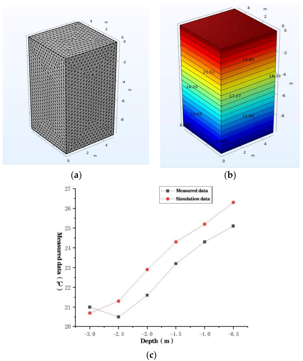
2.6.1. Grid Division

Due to the considerable variance in size of the model, the breadth of the soil is 15 m and the thickness of the concrete bedding layer is 100 mm; therefore, an inhomogeneous meshing method was adopted. Key study areas, including wall corners and indoor floors, were encrypted with a grid pattern. The model contains a total of 80,842 grids, and the isotherms are smooth and free of jagged edges, as depicted in Figure 4.

2.6.2. Model Settings

In order to improve the simulation’s efficiency, the building model has been appropriately simplified. The building model is a 10 m long, 10 m wide, two-story residential structure. Figure 4b depicts a portion of the structure. The indoor and outdoor temperatures, the thermal properties of the floor and exterior walls, the intensity of outside solar radiation, and the depth and temperature of the soil layer of constant temperature influence the heat transmission from the ground floor. Therefore, the sections of the model that do not affect the inner surface temperature of the corners were eliminated, leaving only the ground floor of the building. As there are no other structures in the vicinity of the model, the influence of the building’s direction on the solar radiation is disregarded, and the solar radiation is simplified to the horizontal plane. Due to the symmetry of heat transfer, just a quarter of the building’s ground floor is modeled. This is seen in Figure 4c. Only the structural and insulation layers of the exterior walls and floors are modeled. The interior and external finishes of the external and internal walls are eliminated since they have little impact on heat transfer. The model keeps the exterior walls’ 1.2 m height. The building’s foundation consists of a 300 mm thick reinforced concrete mat. The exterior walls are comprised of 200 mm thick hollow block and 300 mm thick EPS insulation panels. The proportions of the model’s natural soil are 15 m long, 15 m wide, and 9.62 m deep.

In order to validate the efficacy of the intended combination construction, the combined construction was separated by component and divided into three distinct models, as indicated in Figure 5 shows the IHEB model (model group C) and the VIRL model (model groups D and E). In conjunction with the design of the integrated construction, the traditional energy-efficient building was also modeled by installing insulation within 2 m of the perimeter wall and establishing a group A model. The ICWC model was configured as a group F model. The precise construction of each model group, the working condition grouping, and naming criteria are displayed in

Table 1. Working conditions’ settings and simulation parameters.

Condition No.	Model Grouping	Model Parameters	Variable Values
A1	Group A	$\mathrm{Insulation} \mathrm{layer} \mathrm{laid} \mathrm{within} 2 \mathrm{m} \mathrm{of} \mathrm{the} \mathrm{perimeter} \mathrm{ground} \mathrm{with} \mathrm{a} \mathrm{thickness} \mathrm{of} H_{\mathrm{A}}$.	$H_{\mathrm{A}}=100 mm$
B1~B16	Group B	$\mathrm{The} \mathrm{entire} \mathrm{floor} \mathrm{is} \mathrm{covered} \mathrm{with} \mathrm{insulation}. \mathrm{The} \mathrm{thickness} \mathrm{of} \mathrm{the} \mathrm{insulation} \mathrm{is} \mathrm{indicated} \mathrm{by} H_B$.	$H_B=n20\left(n=0,1,2···15\right)$
C1~C16	Group C	$\mathrm{Add} \mathrm{IHEB} \mathrm{to} \mathrm{the} \mathrm{optimal} \mathrm{working} \mathrm{conditions} \mathrm{of} \mathrm{the} \mathrm{group} \mathrm{B} \mathrm{model}. \mathrm{The} \mathrm{length} \mathrm{of} \mathrm{the} \mathrm{extension} \mathrm{band} \mathrm{is} L_C$.	$L_C=n200\left(n=0,1,2···15\right)$
D1~D17	Group D	$\mathrm{VIRL} \mathrm{is} \mathrm{added} \mathrm{to} \mathrm{the} \mathrm{optimal} \mathrm{working} \mathrm{conditions} \mathrm{of} \mathrm{the} \mathrm{group} \mathrm{B} \mathrm{model}. \mathrm{The} \mathrm{height} \mathrm{of} \mathrm{the} \mathrm{reinforcement} \mathrm{layer} \mathrm{is} L_D.$	$L_D=n50\left(n=0,1,2····16\right)$
E1~E7	Group E	$\mathrm{Combining} \mathrm{the} \mathrm{best} \mathrm{working} \mathrm{conditions} \mathrm{for} \mathrm{the} \mathrm{group} \mathrm{B} \mathrm{and} \mathrm{E} \mathrm{models}, \mathrm{varying} \mathrm{the} \mathrm{thickness} \mathrm{of} \mathrm{the} \mathrm{VIRL}. \mathrm{The} \mathrm{thickness} \mathrm{is} \mathrm{denoted} \mathrm{by} H_E$.	$H_E=n50\left(n=0,1,2····6\right)$
F1	Group F	The optimal conditions of the models in groups B, C, D, E are combined to form the group F model.

, and Figure 5 depicts the specific construction design.

2.7. Thermophysical Properties of Materials

Table 2. Thermophysical properties of materials.

Name of Material	Application Area	Thermal Conductivity W/(m·K)	Specific Heat Capacity kJ/(kg K)	Density kg/m3
Reinforced concrete	Mat foundation	1.74	0.92	2500
Extruded polystyrene board	Floor insulation	0.032	1.38	35
Expanded polystyrene board	External wall insulation	0.039	1.38	20
Hollow block	Facade walls	0.74	-	1520
Silty clay	Soil	0.58	1.01	13.44

displays the thermophysical parameters of the materials used in the simulation. The experimental site was created in preparation for the construction of an ultra-low energy building. A geological survey was commissioned for the construction site. The Ground Investigation Report indicates that the experimental site’s soil is a silty clay. The current Chinese national standard [42] stipulates that the thermal conductivity of silty clay is 0.58 W/(m·K), the thermal storage coefficient is 7.69 W/(m²·K), and the specific heat capacity is 1.01 kJ/(kg·K).

2.8. Validation of CFD Simulation Analysis

Numerous investigations have validated the CFD simulation of heat transfer in enclosures. However, there are fewer soil CFD modeling use cases. Further validation is required to determine whether or not it can objectively reflect soil heat transport. In this investigation, CFD simulation methodologies were validated using field experiments. A section of natural soil was selected for manual excavation at a construction site within a factory in Changchun, China. The excavated pit was 2 m wide, 2 m long, and 3 m deep. A probe thermometer was arranged at 0.5 m intervals, with a total of 6 set up. With a range of −50 °C to 199 °C, the probe-type thermometer chosen measures thermocouple contact. The accuracy is 1 °C, and the resolution is 0.1 °C. The error of the validation experiment is estimated to be 1 °C. The error of the CFD simulation experiment is estimated to be 0.1 °C. After 48 h of backfilling and stabilization, data were captured together with the prevailing environmental data. The temperature information is presented in

Table 3. Comparison table of measured and simulated data.

Name of Material	Depth (m)	Equipment Readings (°C)	Simulation Data (°C)	Error (°C)
Thermometer 1	−0.5	25.1	26.3	1.2
Thermometer 2	−1.0	24.3	25.2	−0.9
Thermometer 3	−1.5	23.2	24.3	−1.1
Thermometer 4	−2.0	21.6	22.9	−1.3
Thermometer 5	−2.5	20.5	21.3	−0.8
Thermometer 6	−3.0	21.0	20.7	0.3

.

According to the previous calculation, the depth of the soil layer of constant temperature in Changchun is 9.62 m. In the simulation, a 5-by-5-by-9.62 m soil model was used. The model’s surrounding boundary conditions were symmetrical. The temperature of the soil layer of constant temperature was 6.1 °C. The simulated meteorological data utilized actual data from the day of the experiment. The dry bulb temperature was 22.9 °C, the horizontal solar radiation was 138.89 W/m², and the wind speed was 9 m/s. Figure 6 displays the partition of the model grid and simulation results. Table 3 contains the data generated via simulation.

The mean value of the simulated data was 1.1 °C higher than the mean value of the actual data, with a range between 1.2 °C and 0.2 °C. On average, the standard deviation was 4.9%. The greater the soil depth, the smaller the error. The smaller the soil depth, the larger the error. The hypothesized explanation for this inaccuracy is because water evaporation from shallow soils absorbs heat. This is not accounted for by the CFD simulation. However, the error range is within acceptable parameters, and the trend in temperature corresponds well with actual measurements. Figure 5 displays the trend of temperature. Consequently, the CFD simulation method is relevant to this investigation.

3. Results

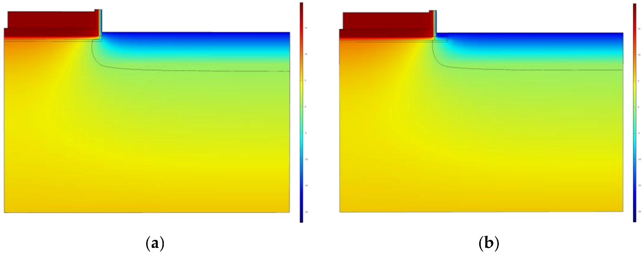
3.1. Simulation Results with the Entire Floor Covered with Insulation (Group B)

3.1.1. The Function of Full Floor Insulation

Due to the constant room temperature in the simulation, the change in temperature of the inner surface of the ground does not visually reflect the heat transfer from the underlying structure. The soil temperature beneath the structure is a good visual representation of the heat transfer from the earth. The surrounding environment influences the temperature of the earth beneath the building, and the amount of heat emitted is rather constant. The higher the temperature, the greater the heat transmission from the earth, but the lower the temperature, the less heat transfer.

Table 4. Temperature distribution of B1, A1, and B6 working conditions.

	B1 Working Conditions	A1 Working Conditions	B6 Working Conditions
Temperature simulation results
Simulation results for reduced temperature range

compares the simulation results for the three different scenarios: B1 (no ground insulation), A1 (conventional energy-efficient building with insulation within 2 m of the perimeter ground), and B6 (no ground insulation) (120 mm thick GFIL). The third row in Table 4 displays the temperature as a range reduction to make it easier to compare changes in the minimum temperature of the interior surface. The simulation results for the 16 models in group B are displayed in Figure 7a–p. It is easier to see how the soil’s temperature changed beneath the structure.

As shown in Table 4 and Figure 7, the B6 working condition of the GFIL substantially reduces heat transfer from the ground to the soil below. The average soil temperature within two meters of the building is only 5.13 °C, a decrease of 6.07 °C compared to the B1 working condition and 2.68 °C compared to the A1 working condition. As depicted in Figure 4 and Figure 7, as the ground insulation was increased, the average soil temperature within 2 m of the building gradually reduced, with a maximum decline of 8.8856 °C from 11.196 °C to 2.3104 °C. The decline was almost 79.4%. This demonstrates that GFIL can significantly limit the heat transmission from the indoor floor to the soil below. The average temperature of the earth beneath the floor drops at a slower rate as the thickness of the insulation increases. The GFIL is too thick and does not provide additional energy savings benefits, but rather increases economic costs and carbon emissions.

The group B model’s simulation results are shown in Figure 8 and

Table 5. Simulation results for Group A and B working conditions.

Condition No.	Temperature Minimum on Inner Surface (°C)	Average Temperature of the Inner Surface (°C)	Average Temperature of the Soil Within 2 m Below the Building (°C)
A1	16.25	19.39	7.81
B1	13.33	18.96	11.20
B2	15.01	19.22	9.14
B3	15.58	19.32	7.70
B4	15.90	19.39	6.63
B5	16.10	19.44	5.80
B6	16.24	19.48	5.13
B7	16.34	19.52	4.59
B8	16.42	19.54	4.14
B9	16.48	19.57	3.77
B10	16.52	19.59	3.45
B11	16.56	19.61	3.18
B12	16.59	19.62	2.95
B13	16.62	19.63	2.75
B14	16.64	19.64	2.58
B15	16.66	19.66	2.44
B16	16.67	19.67	2.31

. The three curves depict the link between GFIL and the inner surface’s minimum temperature, average temperature, and soil temperature in the two meters below building surface. The curves’ general trend agrees with the results of the prior investigation. The curves in Figure 8 can be used to learn it. A thickness of 200–240 mm is more appropriate for GFIL in cold areas (XPS).

As illustrated in Table 4, the temperature representation of the simulation data is compressed so that distinct low-temperature zones are visible at the wall’s roots and corners. The GFIL and perimeter floor paving insulation can make the low temperature phenomenon at the wall’s roots and corners much weaker, but it cannot be eradicated entirely, especially at the corner site. For A1 and B6 working conditions, the lowest surface temperatures on the exterior of the walls were 16.25 °C and 16.24 °C, respectively.

3.1.2. Low Temperature at the Roots and Corners of Walls

Figure 7q–s show the simulation results of heat flow at the wall corners for B1, A1, and B6 operating conditions. For simulation results with the lowest temperatures, it can be seen that the GFIL increases the temperature of the inner surface face at the corner. The additional 60 mm of insulation raises the corner temperature by 2.57 °C, from 13.330 °C to 15.900 °C. Increasing the thickness of the insulation marginally raises the temperature. The simulation findings for 300 mm of insulation versus 100 mm of insulation resulted in a 0.43 °C rise in the internal surface temperature. Despite the fact that the GFIL has increased the ground temperature, the temperature at the wall’s corner is still much lower than the average indoor temperature and the ground temperature. There is currently no specific temperature restriction in China for the inside surface of the envelope, which just needs to be devoid of condensation. However, international requirements for low-energy buildings require that the difference in temperature between the inner surface of the envelope and the internal temperature not exceed 3 °C. When the temperature difference surpasses 3 °C, condensation and mold are likely to form in environments with high humidity. Looking at Figure 7, it can be determined from Figure 7q–s that the previously analyzed heat transport from the ground is broadly compatible with the simulated scenario. The heat flow is from the high-temperature region to the low-temperature region, and it is most intense at the corners of the building’s outer walls. Neither pavement insulation within two meters of the perimeter floor nor GFIL can effectively resolve this issue.

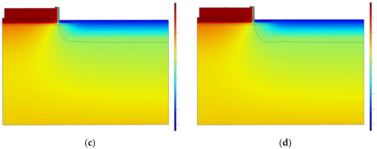
3.2. Simulation Results for the Insulated Horizontal Extension Belt Configuration (Group C)

As seen in

Table 6. Simulation results for Group C working conditions.

Condition No.	Temperature Minimum on Inner Surface (°C)	Average Temperature of the Inner Surface (°C)	Average Temperature of the Soil Within 2 m Below the Building (°C)
C1	16.56	19.61	3.18
C2	16.58	19.61	3.53
C3	16.60	19.62	3.85
C4	16.61	19.62	4.11
C5	16.63	19.63	4.31
C6	16.64	19.63	4.46
C7	16.65	19.63	4.58
C8	16.66	19.63	4.68
C9	16.66	19.63	4.75
C10	16.67	19.63	4.81
C11	16.67	19.64	4.85
C12	16.67	19.64	4.89
C13	16.68	19.64	4.91
C14	16.68	19.64	4.93
C15	16.68	19.64	4.95
C16	16.68	19.64	4.96

, the IHEB can play a role in improving the average ground temperature, the lowest temperature value at the corner, and the soil temperature beneath the building, and the trend of improvement is more consistent. However, the average temperature of the inner surface and the low temperature at the wall’s corner are only marginally increased. The simulation results of the group C model are shown in Figure 9 plotted against the inner surface’s minimum temperature, average temperature, and soil temperature within two meters of the building. As depicted in Figure 9, the IHEB has a minor increase in the average temperature of the inner surface of the floor and a low temperature at the wall corner. The IHEB was laid over a distance of 3 m. However, the temperature increase at the corner of the wall was only 0.119 °C, which is not a satisfactory solution to the problem of low internal surface temperature at the corner of the wall.

3.3. Results of VIRL Simulations (Groups D and E)

As demonstrated in

Table 7. Simulation results for Group D and E working conditions.

Condition No.	Temperature Minimum on Inner Surface (°C)	Average Temperature of the Inner Surface (°C)	Average Temperature of the Soil Within 2 m Below the Building (°C)
D1	16.62	19.64	3.12
D2	16.65	19.64	3.15
D3	16.69	19.64	3.17
D4	16.74	19.65	3.20
D5	16.80	19.65	3.22
D6	16.84	19.66	3.22
D7	16.94	19.66	3.23
D8	17.05	19.67	3.28
D9	17.12	19.67	3.25
D10	17.24	19.68	3.25
D11	17.37	19.68	3.25
D12	17.41	19.69	3.25
D13	17.47	19.69	3.26
D14	17.54	19.69	3.26
D15	17.58	19.70	3.26
D16	17.63	19.70	3.26
D17	17.67	19.70	3.26
E1	16.62	19.63	2.75
E2	16.99	19.66	2.81
E3	17.17	19.68	3.68
E4	17.29	19.68	3.11
E5	17.37	19.68	3.25
E6	17.41	19.69	3.40
E7	17.45	19.69	3.46

, the VIRL significantly improves the low temperature at the wall’s corner. The minimum temperature at the wall’s corner is increased by 1.043 °C to 17.671 °C when the height of VIRL is 800 mm. When the thickness of VIRL is 200 mm and the height is 350 mm, the requirement that the temperature of the inner surface of the envelope must not be lower than the indoor temperature by 3 °C can be met. If greater insulation is desired, a height of 500 mm is more acceptable.

By altering the thickness of the VIRL, the group E model has evolved from the D11 model. The heat flow density analysis for the B1, E4, and E7 working conditions is shown in Figure 10. The heat flow will be from indoor to outdoor through the corner in the B1 case in the figure because there is no VIRL added. The corner’s thermophysical characteristics will be significantly enhanced by the VIRL in the E4 case. E4 will significantly reduce the heat flow density at the corner compared to the B1 case and will also be the edge length of the heat flow transfer path from the interior ground. The heat flow will be transferred from the interior to the soil under the building and then to the outdoor soil. The VIRL lets the dense heat flow from the corners of the walls migrate outwards, thereby increasing the internal surface temperature at the corners and roots of the walls. At 200 mm, the VIRL is 0.38 °C higher than at 50 mm. At an indoor temperature of 20 °C, a 100 mm thick VIRL can raise the corner temperature above 17 °C. Figure 11 depicts the relationship between the inner surface’s minimum temperature and the height and thickness of the VIRL. As can be seen, there is essentially a diagonal relationship between the height of VIRL and the minimum surface temperature. An upward convex curve represents the relationship between the VIRL thickness and the inner surface’s minimum temperature. This shows that the temperature increase of the inner surface becomes smaller and smaller as the VIRL thickness increases. Figure 11 demonstrates that the VIRL at 150–200 mm provides superior insulation without increasing insulating material waste.

3.4. Optimization of ICWC

By comparing data from the simulation results, the optimal working conditions from the models of groups B, C, D, and E were combined to form the model of group F. The GFIL has a thickness of 240 mm, the IHEB has a length of 800 mm and a thickness of 240 mm, and the VIRL has a height of 500 mm and a thickness of 150 mm.

As shown in

Table 8. Comparison of Group F models with other optimal models.

Condition No.	Temperature Minimum on Inner Surface °C	Average Temperature of the Inner Surface °C	Average Temperature of the Soil Within 2 m Below the Building °C
A1	16.25	19.39	7.81
F1	17.35	19.69	4.42
B13	16.62	19.63	2.75
C5	16.63	19.63	4.31
E4	17.29	19.68	3.11

, the simulations result for all group F model indicators exceeded the optimal working conditions model for each group. The lowest temperature of the inner surface at the corner of the wall for the group F model was 17.349 °C, an increase of 0.059 °C from the E3 working condition and 0.732 °C from the B13 working condition. In addition, the average soil temperature rose by 0.117 °C in comparison to the C5 condition. With the call to reduce carbon emissions and save materials, the ICWC of the group F model can more effectively solve the problem of low internal surface temperatures at the corners of the walls, as well as raise the soil temperature beneath the building, resulting in a substantial reduction in heat transfer from the interior to the exterior.

4. Discussion

This study aims to meet the criteria of ultra-low energy buildings by optimizing energy-saving approaches for corner enclosures in order to eliminate excessively low temperatures on their internal surfaces and enhance indoor comfort. This study’s findings and techniques can therefore be used as references and guidelines for the design and retrofitting of ultra-low energy buildings in extreme cold climates.

4.1. Regression Analysis

It is vital to investigate the process by which ICWC increases the interior surface temperature, so we conducted the required regression analysis on the findings of the experiment. This can help to clarify how ICWC operates. Additionally, it makes it possible to understand IHEB, VIRL, and GFIL’s roles and functions more intuitively.

The correlation between the variables in each group of models and the outcomes of the three simulations was the first analysis carried out (inner surface temperature minimum, ground temperature mean, and bottom soil temperature mean).

Table 9. Pearson correlation coefficient.

Variables of Models (mm)	Temperature Minimum on Inner Surface	Average Temperature of the Inner Surface	Average Temperature of the Soil Within 2 m Below the Building
$H_B$	$\mathsf{\gamma } =$ 0.768	$\mathsf{\gamma } =$ 0.887	$\mathsf{\gamma } =$ −0.923
$L_C$	$\mathsf{\gamma } =$ 0.927	$\mathsf{\gamma }=$ 0.908	$\mathsf{\gamma } =$ 0.906
$L_D$	$\mathsf{\gamma } =$ 0.992	$\mathsf{\gamma } =$ 0.993	$\mathsf{\gamma } =$ 0.886
$H_E$	$\mathsf{\gamma } =$ 0.922	$\mathsf{\gamma } =$ 0.870	$\mathsf{\gamma } =$ 0.650

displays the analysis’ findings.

The Pearson correlation coefficient in statistics calculates the linear correlation.

It is determined using Equation (9).

$$\mathsf{\gamma }=\frac{1}{\mathrm{n}-1}{{\displaystyle \sum }}_{i=0}^n\left(\frac{x_i-\overline{x}}{{\sigma }_x}\right){\left(\frac{y_i-\overline{y}}{{\sigma }_y}\right)}^{ }$$

(9)

$\mathsf{\gamma }$ in the formula is the sample correlation coefficient. $x_i$ and $y_i$ are the coordinate values of the sample points. $n$ is the number of samples. $\frac{x_i-\overline{x}}{{\sigma }_x}$ and $\frac{y_i-\overline{y}}{{\sigma }_y}$ are the standard scores of $x_i$ and $y_i$, respectively. $\overline{x}$ and $\overline{y}$ are the sample means. ${\sigma }_x$ and ${\sigma }_y$ are the sample standard deviations.

The correlation is stronger when the correlation coefficient is greater in absolute value, closer to 1 or −1, stronger when the correlation coefficient is smaller, and weaker when the correlation coefficient is smaller.

Table 9 shows that for the temperature minimum on the inner surface, the correlations of the variables for all four groups of models are positive. This means that as the variables rise, the minimum surface temperature also rises. It can also be inferred that as the four groups of models perform better, the minimum value of the inner scale temperature will also rise in line with that. $H_E$ is the one with the biggest impact, followed by $L_C$ and $L_D$. The effect of $H_B$ is the smallest. This shows that the thickness of GFIL ($H_B$) has the least impact on the inner surface temperature, whereas the height of VIRL ($L_D$) has the greatest impact. The average temperature of the inner surface showed a positive correlation with all four variables. $L_D$ and $L_C$ have the best correlations. In comparison to $L_D$ and $L_C$, the correlation between $H_B$ and $H_E$ is not significantly different and is even lower. Consequently, it is understood that the most significant factor is still the thickness of the VIRL ($L_D$). Therefore, it can be concluded that VIRL has a significant impact on the rise in the internal surface temperature. IHEB and GFIL did play a supporting role, though, and that cannot be disregarded. It is also known that when compared to the correlation of the temperature minimum on the inner surface, the correlation of the average temperature on the inner surface of $H_B$ increases by 0.12 units. Although GFIL does not have a significant impact on the inner surface temperature’s minimum value, it does have a significant impact on its mean value, which is essentially the same as IBEB’s impact.

Positive correlations existed between $L_C$, $L_D$, $H_E$, and average soil temperature within 2 m beneath the building. The correlation between $L_C$ and $H_E$ was 0.91 for $L_C$ and 0.65 for $H_E$, respectively. For $H_B$, the correlation was −0.92. This shows that $H_B$ causes a significant decrease in the average soil temperature within 2 m below the building, while other factors raise this temperature. This is due to the fact that GFIL reduces heat transfer from the interior to the soil beneath the building, resulting in a drop in soil temperature.

Multiple Regression Analysis

Multiple regression analysis is a statistical analysis method that considers one variable as the dependent variable and one or more other variables as the independent variables in the variables of interest, and establishes a linear or nonlinear mathematical model quantitative relationship between multiple variables and analyses them using sample data. Multiple regression analysis of the results of this experiment can simplify the more complex working mechanism of ICWC into an intuitive empirical formula. In environments with more comparable climatic conditions, the empirical equation can be used directly to estimate corner insulation performance. The architectural design could benefit greatly from this work.

$H_B$, $L_C$, $L_D$, and $H_E$ are the independent variables in the multiple regression experiment. Temperature minimum on inner surface, the average temperature of the inner surface, and the average temperature of the soil within 2 m below the building are the dependent variables. Equations (10)–(12) provide the empirical formulas for each dependent variable and each independent variable.

$$t_{\mathrm{M}}=15.082+\left(7H_B+L_D\right)/1000$$

(10)

$$t_{\mathrm{A}}=19.227+\left(2H_B+0.024L_C+0.068L_D+0.041H_E\right)/1000$$

(11)

$$t_{\mathrm{S}}=8.644+\left(-25H_B+L_C\right)/1000$$

(12)

In the equation, $t_{\mathrm{M}}$ is the temperature minimum on the inner surface. $t_{\mathrm{A}}$ is the average temperature of the inner surface. $t_{\mathrm{S}}$ is the average temperature of the soil within 2 m below the building. $H_B$ is the thickness of GFIL (mm). $L_C$ is the length of IHEB (mm). $L_D$ is the height of VIRL (mm). $H_E$ is the thickness of VIRL (mm).

4.2. IHEB’s Function

IHEB’s function is a major crucial aspect. The simulation results reported in Section 3 demonstrate that the IHEB results in a more significant increase in the soil temperature beneath the structure, without increasing the heat transfer from the interior to the soil below the building. With a 1.2 m long IHEB, the average soil temperature within two meters of the building is 1.4017 °C higher than without the extension strip. Simultaneously, the IHEB relocates the 0 °C isotherm of the soil beneath the building.

Figure 12 shows the simulation results of the 0 °C isotherm positions for the C1, C4, C7, and C9 operating conditions. The figure shows that the 0 °C isotherm for C1 and C4 conditions is still partially below the building. The 0 °C isotherms for the C7 and C9 conditions are completely out of the building. This indicates that the 0 °C isotherm will gradually move away from the building as the length of IHEB increases. At IHEB lengths longer than 800 mm, the soil temperature beneath the building’s main body is over the 0 °C isotherm, indicating that the soil is not frozen. The effect of the IHEB on the soil beneath the building’s main body will not only reduce the building’s energy consumption but will also alter the building’s foundation depth. In colder climates, structures are typically buried deeper than the depth of the local permafrost. A properly installed IHEB allows the impact of permafrost on the building foundation to be ignored and just the bearing capacity of the soil on the foundation to be evaluated, which can greatly reduce the amount of excavation necessitated by the permafrost issue. IHEB construction is also ideally suited for temporary buildings, such as dormitories for construction workers and houses for disaster assistance, which may be constructed with remarkable rapidity.

The envisaged ICWC is derived from the common ground insulation extension construction of ultra-low energy buildings and combines it with the practice of cold gutter insulation construction. It has been demonstrated that the ICWC raises the internal surface temperature; however, some issues remain unresolved. First, the ICWC is overly thick in some places. This causes the material to easily distort following freeze–thaw cycles, and its durability is compromised. Second, the IHEB will prevent the soil beneath the building from freezing, but the soil in front of the IHEB will attain temperatures below 0 °C. This implies that the IHEB requires additional frost-resistant construction to prevent distortion and damage caused by freezing and expansion. Thirdly, the simulation studies conducted to date are still relatively limited to seasonally frozen soil areas, and it is necessary to conduct additional testing to see whether the developed structure is appropriate in other cold places. These are also the most important concerns that must be investigated in the future.

5. Conclusions

As a major energy user, it is vital to minimize energy consumption in buildings, and promoting ultra-low energy buildings aggressively is unquestionably a potent strategy for doing so. The extremely low energy consumption levels and severe construction criteria of ultra-low energy buildings exert more demands on the envelope system. In this study, CFD modeling was employed to simulate the corner wall envelope of an ultra-low energy structure, and a comparative method was employed to validate the performance of the constructed ICWC. In addition, the applicability of the CFD simulation method to this study was confirmed, and it was proved that the experimental results were not affected by the margin of error. By dividing the planned ICWC model into five groups and comparing them to conventional energy-efficient building floor insulation structures, a total of 58 models were analyzed. The following are the study’s findings:

• GFIL can significantly reduce heat transfer from a building’s interior to the soil below. When GFIL’s XPS panels are 240 mm thick, the soil temperature within 2 m of the building is 2.75 °C, a drop of 5.06 °C compared to typical perimeter floor layer insulation. Compared to an uninsulated structure, a reduction of 8.44 °C is observed.
• Incorporate IHEB in GFIL. The longer the IHEB, the less heat is transported from the soil beneath the building to the surrounding soil, resulting in an increase in temperature. When the IHEB is 800 mm long, the average soil temperature beneath the building is 1.13 °C higher than when there is no IHEB. When the IHEB is 3000 mm long, the average soil temperature within two meters of the building rises by 1.78 °C. Following analysis, an IHEB length of 800 mm is deemed suitable.
• In seasonally frozen areas, a reasonable arrangement of the insulation IHEB allows the soil temperature underneath the building to be above 0 °C and not freeze. Under the boundary conditions chosen in the simulations, the soil temperature below the building was above 0 °C when the IHEB length was 800 mm.
• Traditional perimeter ground insulation, the GFIL, and the IHEB do not resolve the problem of low internal surface temperatures at the roots and corners of walls.
• The VIRS was successful at increasing the internal surface temperature of the wall’s base and corners. In the test scenario, the 500 mm tall and 150 mm thick VIRS was the most cost-effective and appropriate solution. It increased the surface temperature to 17.29 °C.
• The designed ICWC improves the interior surface temperature of the corner and also possesses the benefits of models in groups C and D. The optimal performance of the ICWC is achieved with a 240 mm thick GFIL, an 800 mm long IHEB, and a 500 mm tall and 150 mm thick VIRL. It can reach an internal surface temperature of 17.35 °C at the corner, a ground temperature of 19.69 °C on average, and a soil temperature of 4.42 °C on average within −2 m below the building, which is superior to the performance of the other three sets of models operating independently.

Through CFD simulation analysis, the designed ICWC improves the overall thermophysical properties of the ground, reduces the heat transferred out, and further reduces the energy consumption of the building. It also solves the problem of low internal surface temperature at the corners and roots of walls in seasonally frozen soil regions, which makes them prone to condensation and mold. IHEB raises the temperature of the soil beneath and around the building floor. This allows the building to be constructed without regard to the effects of seasonal frost and can reduce the depth of burial of the building. It also provides a new vision for decreasing the amount of foundation trench earthwork necessary in seasonally frozen soil regions and for the speedy construction of emergency homes.

References

1. Perez, M.; Perez, R. Update 2022–A fundamental look at supply side energy reserves for the planet. Sol. Energy Adv. 2022, 2, 100014. [Google Scholar] [CrossRef]
2. Way, R.; Ives, M.C.; Mealy, P.; Farmer, J.D. Empirically grounded technology forecasts and the energy transition. Joule 2022, 6, 2057–2082. [Google Scholar] [CrossRef]
3. Żywiołek, J.; Rosak-Szyrocka, J.; Khan, M.A.; Sharif, A. Trust in renewable energy as part of energy-saving knowledge. Energies 2022, 15, 1566. [Google Scholar] [CrossRef]
4. Yang, X.; Zhang, S.; Xu, W. Impact of zero energy buildings on medium-to-long term building energy consumption in China. Energy Policy 2019, 129, 574–586. [Google Scholar] [CrossRef]
5. Schwartz, L.C.; Miller, C.; Murphy, S.; Frick, N.M. State Indicators for Advancing Demand Flexibility and Energy Efficiency in Buildings-Part I; Lawrence Berkeley National Laboratory (LBNL): Berkeley, CA, USA, 2022. [Google Scholar]
6. Chen, Y. Chinese solutions and contributions to the global response to climate change. Contemp. World 2021, 5, 4–9. [Google Scholar]
7. Mengis, N.; Kalhori, A.; Simon, S.; Harpprecht, C.; Baetcke, L.; Prats-Salvado, E.; Schmidt-Hattenberger, C.; Stevenson, A.; Dold, C.; El Zohbi, J. Net-Zero CO2 Germany—A Retrospect from the Year 2050. Earth’s Future 2022, 10, e2021EF002324. [Google Scholar] [CrossRef]
8. Ahmed, Z.; Cary, M.; Ali, S.; Murshed, M.; Ullah, H.; Mahmood, H. Moving toward a green revolution in Japan: Symmetric and asymmetric relationships among clean energy technology development investments, economic growth, and CO2 emissions. Energy Environ. 2022, 33, 1417–1440. [Google Scholar] [CrossRef]
9. Kim, J.T.; Yu, C.W.F. Sustainable development and requirements for energy efficiency in buildings–the Korean perspectives. Indoor Built Environ. 2018, 27, 734–751. [Google Scholar] [CrossRef]
10. Ascione, F.; De Masi, R.F.; de Rossi, F.; Ruggiero, S.; Vanoli, G.P. Optimization of building envelope design for nZEBs in Mediterranean climate: Performance analysis of residential case study. Appl. Energy 2016, 183, 938–957. [Google Scholar] [CrossRef]
11. Congedo, P.M.; Baglivo, C.; Seyhan, A.K.; Marchetti, R. Worldwide dynamic predictive analysis of building performance under long-term climate change conditions. J. Build. Eng. 2021, 42, 103057. [Google Scholar] [CrossRef]
12. Albatayneh, A. Sensitivity analysis optimisation of building envelope parameters in a sub-humid Mediterranean climate zone. Energy Explor. Exploit. 2021, 39, 2080–2102. [Google Scholar] [CrossRef]
13. Ashhar, M.Z.M.; Haw, L.C. Recent research and development on the use of reflective technology in buildings–A review. J. Build. Eng. 2022, 45, 103552. [Google Scholar] [CrossRef]
14. Jankovic, A.; Goia, F. Control of heat transfer in single-story mechanically ventilated double skin facades. Energy Build. 2022, 271, 112304. [Google Scholar] [CrossRef]
15. Pan, L.; Xu, Q.; Nie, Y.; Qiu, T. Analysis of climate adaptive energy-saving technology approaches to residential building envelope in Shanghai. J. Build. Eng. 2018, 19, 266–272. [Google Scholar] [CrossRef]
16. 1Zhou, Z.; Wang, C.; Sun, X.; Gao, F.; Feng, W.; Zillante, G. Heating energy saving potential from building envelope design and operation optimization in residential buildings: A case study in northern China. J. Clean. Prod. 2018, 174, 413–423. [Google Scholar] [CrossRef]
17. Feng, W.; Huang, J.; Lv, H.; Guo, D.; Huang, Z. Determination of the economical insulation thickness of building envelopes simultaneously in energy-saving renovation of existing residential buildings. Energy Sources Part A Recovery Util. Environ. Eff. 2019, 41, 665–676. [Google Scholar] [CrossRef]
18. Hu, J.; Yu, X. Thermo and light-responsive building envelope: Energy analysis under different climate conditions. Sol. Energy 2019, 193, 866–877. [Google Scholar] [CrossRef]
19. Gagliano, A.; Aneli, S. Analysis of the energy performance of an Opaque Ventilated Façade under winter and summer weather conditions. Sol. Energy 2020, 205, 531–544. [Google Scholar] [CrossRef]
20. Kishore, R.A.; Bianchi, M.V.; Booten, C.; Vidal, J.; Jackson, R. Optimizing PCM-integrated walls for potential energy savings in US Buildings. Energy Build. 2020, 226, 110355. [Google Scholar] [CrossRef]
21. Rathore, P.K.S.; Shukla, S.K.; Gupta, N.K. Potential of microencapsulated PCM for energy savings in buildings: A critical review. Sustain. Cities Soc. 2020, 53, 101884. [Google Scholar] [CrossRef]
22. Homod, R.Z.; Almusaed, A.; Almssad, A.; Jaafar, M.K.; Goodarzi, M.; Sahari, K.S. Effect of different building envelope materials on thermal comfort and air-conditioning energy savings: A case study in Basra city, Iraq. J. Energy Storage 2021, 34, 101975. [Google Scholar] [CrossRef]
23. Vox, G.; Blanco, I.; Convertino, F.; Schettini, E. Heat transfer reduction in building envelope with green façade system: A year-round balance in Mediterranean climate conditions. Energy Build. 2022, 274, 112439. [Google Scholar] [CrossRef]
24. Zhao, J.; Du, Y. A study on energy-saving technologies optimization towards nearly zero energy educational buildings in four major climatic regions of China. Energies 2019, 12, 4734. [Google Scholar] [CrossRef] [Green Version]
25. Zhao, K.; Jiang, Z.; Huang, Y.; Sun, Z.; Wang, L.; Gao, W.; Ge, J. The method of reducing heat loss from thermal bridges in residential buildings with internal insulation in the hot summer and cold winter zone of China. J. Build. Eng. 2022, 62, 105421. [Google Scholar] [CrossRef]
26. Zhang, Y. Floor insulation and energy saving in harsh cold regions. J. Chifeng Coll. Nat. Sci. Ed. 2012, 59–61. [Google Scholar] [CrossRef]
27. Yang, H.; Liu, M.; Jin, F.; Sun, H. A discussion on ways to insulate the touchdown envelope. Build. Sci. 2017, 33, 123–128. [Google Scholar]
28. Bai, Y.; LIU, W.; Chai, Y.; Che, Z.; Tong, G. The effect of chilling furrows on lateral ground temperature in heliostats. J. Shenyang Agric. Univ. 2004, 35, 595–597. [Google Scholar]
29. Alhawari, A.; Mukhopadhyaya, P. Thermal bridges in building envelopes—An overview of impacts and solutions. Int. Rev. Appl. Sci. Eng. 2018, 9, 31–40. [Google Scholar] [CrossRef]
30. Miąsik, P.; Lichołai, L. The influence of a thermal bridge in the corner of the walls on the possibility of water vapour condensation. In Proceedings of the E3S Web of Conferences, Polańczyk, Poland, 19–23 June 2018; p. 00072. [Google Scholar] [CrossRef] [Green Version]
31. Boronbaev, E.; Unaspekov, B.; Abdyldaeva, A.; Tohlukova, E.; Holmatov, K.; Zhyrgalbaeva, N. Full-Fledged Use of Semi-Basement Space by Building Seismic-Resistance, Energy-Efficiency, Microclimate and Preventing Influences of Thermal Bridges and Mold Growth. Civ. Eng. Archit. 2022, 10, 131–143. [Google Scholar] [CrossRef]
32. Pasut, W.; De Carli, M. Evaluation of various CFD modelling strategies in predicting airflow and temperature in a naturally ventilated double skin façade. Appl. Therm. Eng. 2012, 37, 267–274. [Google Scholar] [CrossRef] [Green Version]
33. Nasir, M.H.A.; Hassan, A.S. Thermal performance of double brick wall construction on the building envelope of high-rise hotel in Malaysia. J. Build. Eng. 2020, 31, 101389. [Google Scholar] [CrossRef]
34. Lotfabadi, P.; Hançer, P. A comparative study of traditional and contemporary building envelope construction techniques in terms of thermal comfort and energy efficiency in hot and humid climates. Sustainability 2019, 11, 3582. [Google Scholar] [CrossRef]
35. BC HOUSING. Temperature, Airflow and Moisture Patterns in Attic Roofs; BC HOUSING: Burnaby, BC, Canada, 2020. [Google Scholar]
36. Liu, X.; Xu, M.; Guo, J.; Zhu, R. Numerical study on the energy performance of building zones with transparent water storage envelopes. Sol. Energy 2019, 180, 180–690. [Google Scholar] [CrossRef]
37. Connon, R.; Devoie, É.; Hayashi, M.; Veness, T.; Quinton, W. The influence of shallow taliks on permafrost thaw and active layer dynamics in subarctic Canada. J. Geophys. Res. Earth Surf. 2018, 123, 281–297. [Google Scholar] [CrossRef]
38. Singh, R.K.; Sharma, R.V. Numerical analysis for ground temperature variation. Geotherm. Energy 2017, 5, 22. [Google Scholar] [CrossRef] [Green Version]
39. Brown, J.; Ferrians, O., Jr.; Heginbottom, J.A.; Melnikov, E. Circum-Arctic Map of Permafrost and Ground Ice Conditions; U.S. Department of the Interior: Washington, DC, USA, 1997. [Google Scholar]
40. Li Xin, R.A.N.Y. Frozen Soil Map of China (2000); National Qinghai-Tibet Plateau Scientific Data Center: China, 2016. [CrossRef]
41. Liu, X.; Zhao, C.; Shi, C.; Zhao, B. Study on soil layer of constant temperature. J. Sol. Energy 2007, 28, 5. [Google Scholar] [CrossRef]
42. Ministry of Housing and Urban-Rural Development of the People’s Republic of China (MOHURD). Thermal Design Code for Civil Buildings; China Construction Industry Press: Beijing, China, 2016. [Google Scholar]
43. Administration, C.M. Specialized Meteorological Data Sets for Building Thermal Environment Analysis in China; China Construction Industry Press: Beijing, Chnia, 2015. [Google Scholar]
44. Ministry of Housing and Urban-Rural Development of the People’s Republic of China (MOHURD) Technical Standards for Near-Zero Energy Buildings; China Construction Industry Press: Beijing, China, 2019.
Figure 1. Research methodology flow chart.
Energies 16 01325 g001
Figure 2. (a) Sketch of permafrost variation [37]. (b) Annual Amplitude of Soil Temperature [38]. (c) Soil layer of constant temperature. (d) Northern Hemisphere Permafrost Distribution [39]. (e) Distribution of permafrost types in China [40].
Energies 16 01325 g002aEnergies 16 01325 g002b
Figure 3. Insulation construction of wall corners. (1) Hollow brick walls. (2) Reinforced concrete raft slab foundations. (3) The 200 mm thick EPS board wall external insulation. (4) Concrete bedding. (5) Soil. (7) EPS VIRL. (8) XPS GFIL. (9) XPS IHEB.
Energies 16 01325 g003
Figure 4. (a) Model gridding. (b) Building section diagram. (c) Simulation models.
Energies 16 01325 g004
Figure 5. Model construction for each working condition. (a) Group A model construction. (b) Group B model construction. (c) Group C model construction. (d) Groups D and E models. (e) Group F model construction. (1) Hollow brick walls. (2) Reinforced concrete raft slab foundations. (3) The 200 mm thick EPS board wall external insulation. (4) Concrete bedding. (5) Soil. (6) Ground insulation within 2m of the perimeter of the external wall. (7) EPS VIRL. (8) XPS GFIL. (9) XPS IHEB.
Energies 16 01325 g005
Figure 6. (a) Validation of model meshing. (b) Temperature simulation results. (c) Line graph of measured and simulated data.
Energies 16 01325 g006
Figure 7. Group B model temperature distribution map. (a) Model B1 temperature distribution, (b) Model B2 temperature distribution, (c) Model B3 temperature distribution, (d) Model B4 temperature distribution, (e) Model B5 temperature distribution, (f) Model B6 temperature distribution, (g) Model B7 temperature distribution, (h) Model B8 temperature distribution, (i) Model B9 temperature distribution, (j) Model B10 temperature distribution (k) B11 model temperature profile, (l) B12 model temperature profile, (m) B13 model temperature profile, (n) B14 model temperature profile, (o) B15 model temperature profile, (p) B16 model temperature profile, (q) B1 heat flow direction profile, (r) A1 heat flow direction profile, (s) B6 heat flow direction profile.
Energies 16 01325 g007aEnergies 16 01325 g007b
Figure 8. Thickness of GFIL versus each temperature.
Energies 16 01325 g008
Figure 9. Length of IHEB versus each temperature.
Energies 16 01325 g009
Figure 10. Heat flow density division diagram. (a) B1 heat flow direction diagram, (b) E4 heat flow direction diagram, (c) E7 heat flow direction diagram.
Energies 16 01325 g010
Figure 11. Height and thickness of the VIRL in relation to the minimum ground temperature.
Energies 16 01325 g011
Figure 12. Map of the location of the 0 °C isotherm. (a) Model C1 temperature cloud. (b) Model C4 temperature cloud. (c) Model C7 temperature cloud. (d) Model C9 temperature cloud.
Energies 16 01325 g012aEnergies 16 01325 g012b