Model Predictive Control of DC–DC Boost Converter Based on Generalized Proportional Integral Observer

Abstract

Due to the nonminimum phase characteristics and nonlinearity of boost converters, the control design is always a challenging issue. A novel model predictive control strategy is proposed for the boost converter in this work. First, the Super-Twisting algorithm is applied to current control, and the input–output plant for voltage control is derived based on the linearization technique. All the model uncertainties are defined as lumped disturbances, and a generalized proportional integral observer is designed to estimate the lumped disturbance. Second, a composite predictive approach is developed on the basis of the predictive model and disturbance estimations. By solving the cost function directly, the optimal control law is derived explicitly. Lastly, the effectiveness of the proposed control strategy is verified by both simulation and experimental results.

1. Introduction

The rapid development of the power grid and renewable energy has promoted the extensive application of DC–DC boost converters in various DC voltage conversion occasions, such as uninterruptible power supplies, high-voltage DC (HVDC) power systems, communication equipment, motor drives, fuel cell applications. As a key component in the power conversion system, the output voltage regulation accuracy is particularly important for maintaining a stable bus voltage and achieving satisfactory performance of connected electric equipment [1,2,3]. However, accurate voltage control of the boost-type converter is a rather challenging task due to two major reasons. First, the boost-type converter behaves with nonminimum phase characteristics, and it is intrinsically unstable. Second, the voltage regulation is subject to the adverse effects of system uncertainties, such as dynamic load demand, input voltage change, and other circuit parameter variations. Therefore, it is essential to investigate an effective control law to ensure the performance of the boost converter.

Over the years, several methods have been developed for voltage control. A cascaded PI method was introduced in [4], and another PI method with a low-pass filter was proposed in [5]. High static performance was obtained, whereas the robustness decreased when the converter works at nonnominal points. Said et al. [6] applied fuzzy logic to improve the voltage regulation performance of the boost converter, and the uncertainties were approximated by the Takagi–Sugeno model with 12 affine functions, but the computational burden of the controller was heavy. An internal model control for a boost converter was presented in [7], but it required the inverse of the linear perturbation model, which was complicated in real systems. The backstepping control was presented in [8], but it presented steady-state errors caused by the exact feedback linearization [9]. The sliding mode control is widely employed due to its robustness and fast dynamics, but there is a tradeoff between robustness and chattering [10]. Furthermore, some other methods have been applied to power converters, such as linearization control [11], active disturbance rejection control [12], LQR [13], robust control [14], and intelligent control [15].

Model predictive control (MPC) is a potential candidate for power converters, owing to its optimized tracking performance, fast response, and strong robustness against disturbances [16,17]. The core idea of MPC is to predict the future values of system states and solve the optimization problem defined by different control objectives. According to whether it is an integer optimization program, MPC can be classified into two categories: finite control set MPC (FCS-MPC) and continuous control set MPC (CCS-MPC) [18]. FCS-MPC generates a variable switching frequency and has a higher computational cost than CCS-MPC. Furthermore, CCS-MPC is also superior to FCS-MPC in terms of circuit security and switching loss. Seok et al. [19] employed CCS-MPC for a boost converter to regulate the inductor current, and the dynamic response of current dynamics was improved. However, when designing CCS-MPC as the voltage controller, the main disadvantage that affects control performance is model uncertainties [20]. The integrator is widely used to compensate for model uncertainties, as can be seen in [21] for inverters and in [22] for servo motors. Since the integral control is coupled with other properties, such as dynamic response, stability, and robustness. The utilization of integrators may decrease the other properties of MPC [23]. The online parameter identification methods were also utilized to obtain accurate circuit parameters [24,25]. However, a considerable computational cost was required, and the control accuracy highly depended on the identification accuracy. As a practical solution, disturbance observers were incorporated into MPC works [26,27]. The utilization of disturbance observers can efficiently improve prediction accuracy and enhance robustness. In general, the combination of MPC and observer can be classified into two categories. The first category utilizes the disturbance estimations as a feedforward compensation part of the baseline MPC law [28]. The second category utilizes the estimations to adjust the predictions online and then solved the optimization problem [29]. However, most existing MPC studies assume that the lumped disturbance of the system is fixed in the prediction horizon. In practical systems, the lumped disturbance reflected on power converters is generally a high-frequency and low-frequency mixed time-varying signal, and the trend of the lumped disturbance over the prediction horizon cannot be neglected.

To this end, a novel offset-free CCS-MPC controller is proposed in this paper, and an interleaved boost converter is selected to verify the control performance. The typical dual-loop control framework is adopted, and the Super-Twisting (ST) algorithm is designed for the current control loop, which can guarantee the fast and robust tracking of the given points. The voltage control loop takes advantage of the MPC technique (multiobjective optimization, optimized control effect, etc.), and the time-varying lumped disturbance is considered. The design philosophy is as follows: firstly, a generalized proportional integral observer (GPIO) is constructed to estimate the lumped uncertainties and their derivatives. Secondly, the future output voltage is predicted by a predictive model and disturbance estimations. Lastly, a cost function is designed, and an explicit optimal control law is obtained by solving the cost function directly. Furthermore, strict analysis indicates that the proposed strategy can guarantee the asymptotic stability of the system in the presence of external disturbances and system uncertainties. The main contributions of this paper are summarized as follows:

(1)

The proposed composite MPC with the integrated GPIO achieves offset-free tracking performance under time-varying disturbances.

(2)

The proposed method allows a long prediction horizon, which helps to improve the stability and performance compared with a short prediction horizon.

(3)

Solving the optimization problem online is not required in this paper, as the optimal control law is given explicitly; thus, the online computational burden is limited.

The remainder of this paper is arranged as follows: in Section 2, the system model of the converter is presented; in Section 3, the proposed controller is analyzed in detail; the simulation and experimental results are provided in Section 4 and Section 5; lastly, the conclusions are given in Section 6.

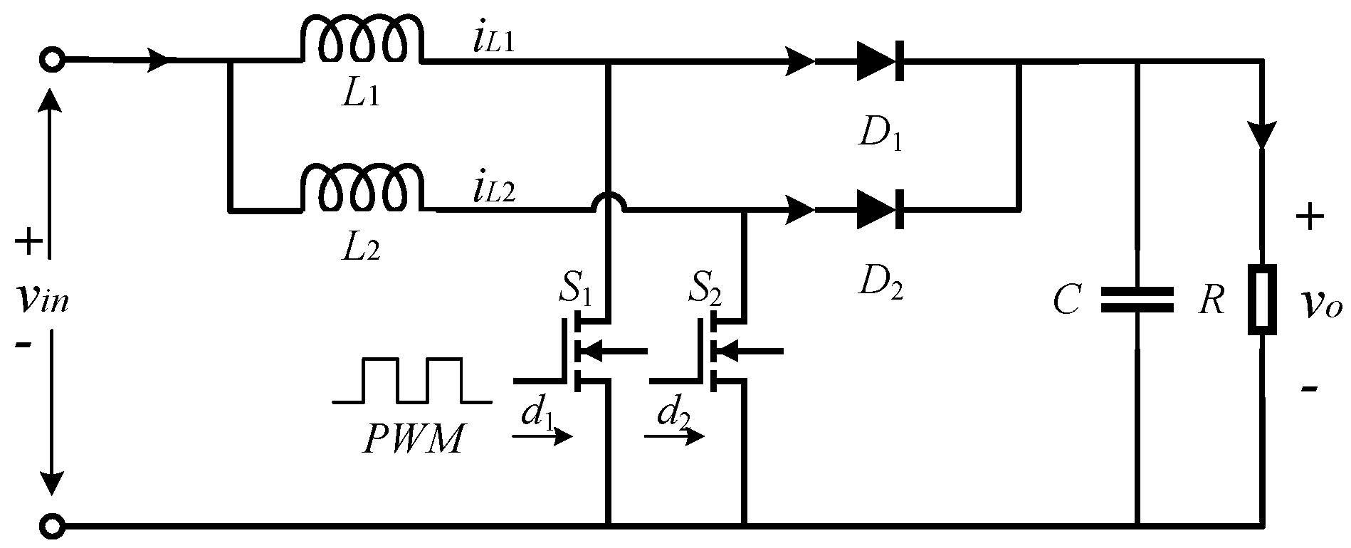
2. Topology Analysis and Modeling

The typical two-phase interleaved boost converter (TIBC) is shown in Figure 1. $L_1,L_2$ are inductors, $C$ is the capacitor, $S_1,S_2$ are MOSFET switches, $D_1,D_2$ are diodes, and $R$ is the equivalent load resistance. $v_{in}$ is the source voltage, $v_o$ is the output voltage, $i_{L1},i_{L2}$ are inductor currents, and $d_1,d_2$ are duty ratios for power switches.

Generally, the circuit parameters of two half-bridge circuits are designed to be the same:

$$L_1=L_2=L,d_1=d_2=d.$$

(1)

Assuming that the converter works in continuous conduction mode, the static model is

$$\left\{\begin{array}{c}{V}_o=V_{in}/\left(1-D\right)\\ I_o=2I_L\left(1-D\right)\end{array}\right.,$$

(2)

where the capital symbols denote the static values of the related system state variables.

According to the average state space technique, the dynamic model of TIBC is

$$L\frac{d{i}_{Li}}{dt}=v_{in}-\left(1-d_i\right)v_o,$$

(3a)

$$C\frac{d{v}_o}{dt}={\displaystyle \sum }\left(1-d_i\right)i_{Li}-\frac{v_o}{R},i=1,2.$$

(3b)

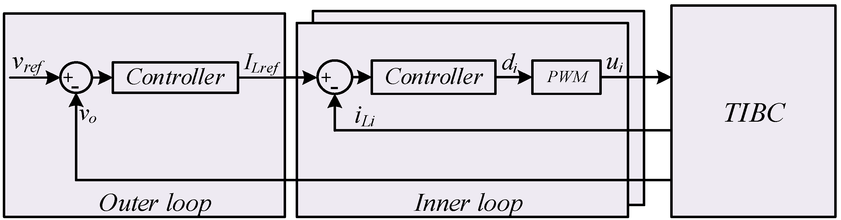
3. Overall Control Strategy

3.1. Current Control

The dual-loop control scheme for power converters is shown in Figure 2. Aiming at the current dynamicsin Equation (3a), the sliding mode surface $s_i$ can be defined as

$$s_i=i_{Li}-I_{Lref},i=1,2,$$

(4)

where $I_{Lref}$ is the reference inductor current.

The ST algorithm is designed as

$$d_i=-\alpha {\left|s_i\right|}^{\frac{1}{2}}sign\left(s_i\right)-\beta \int sign\left(s_i\right)dt,$$

(5)

where α, β are control coefficients, and sign(x) is the sign function.

According to the stability analysis in [30], the current control system will be asymptotically stable if the control parameters satisfy

$$\alpha >L\sqrt{2\epsilon }/v_o,\beta >\left(3{\alpha }^2{v}_o^2\epsilon L+2{\epsilon }^2{L}^3\right)/\left({\alpha }^2{v}_o^3\right),$$

(6)

where $\epsilon$ is defined as $\left|\dot{\kappa }\right|\le \epsilon ,\kappa =\left(v_{in}-v_o\right)/L$.

When the ideal sliding mode (${\dot{s}}_i=s_i=0$) is established, according to Equation (3a), the equivalent control of the current loop is

$$d_{eq}=1+\left(L·d{I}_{Lref}/dt-v_{in}\right)/v_o.$$

(7)

Substituting Equation (7) into Equation (3b), the voltage dynamics is

$$C{v}_o\frac{d{v}_o}{dt}=\left(i_{L1}+i_{L2}\right)\left(v_{in}-L·d{I}_{Lref}/dt\right)-v_o^2/R.$$

(8)

According to Equation (8), the equilibrium point of the system is

$$I_{L1,2}=I_{Lref}=v_o^2/2v_{in}R.$$

(9)

Linearizing Equation (8) around the equilibrium point in Equation (9) gives

$$C{v}_o\frac{d{\tilde{v}}_o}{dt}=2\left(I_L{\tilde{v}}_{in}-L{I}_L·d{\tilde{i}}_L/dt+v_{in}{\tilde{i}}_L\right)-2v_o{\tilde{v}}_o/R.$$

(10)

Therefore, the transfer function from inductor current to output voltage is

$$\left\{\begin{array}{c}{G}_{vi}\left(s\right)=\frac{V_o\left(s\right)}{I_{Lref}\left(s\right)}=\frac{b-cs}{s+a} \\ a=\frac{2}{RC},b=\frac{2v_{in}}{C{v}_o},c=\frac{L{v}_o}{RC{v}_{in}}\end{array}\right..$$

(11)

3.2. Voltage Control

Denoting $I_{Lref}=u,$ and considering the uncertainties of $a,b$ and the right-half plane zero term as the lumped disturbance $f$, the control plant for voltage control is

$${\dot{v}}_o=-a_0{v}_o+b_{0}u+f,$$

(12)

where $a_0,b_0$ can be calculated from Equation (11), and $f=\left(b-b_0\right)I_L-\left(a-a_0\right)v_o-c{\dot{I}}_L$.

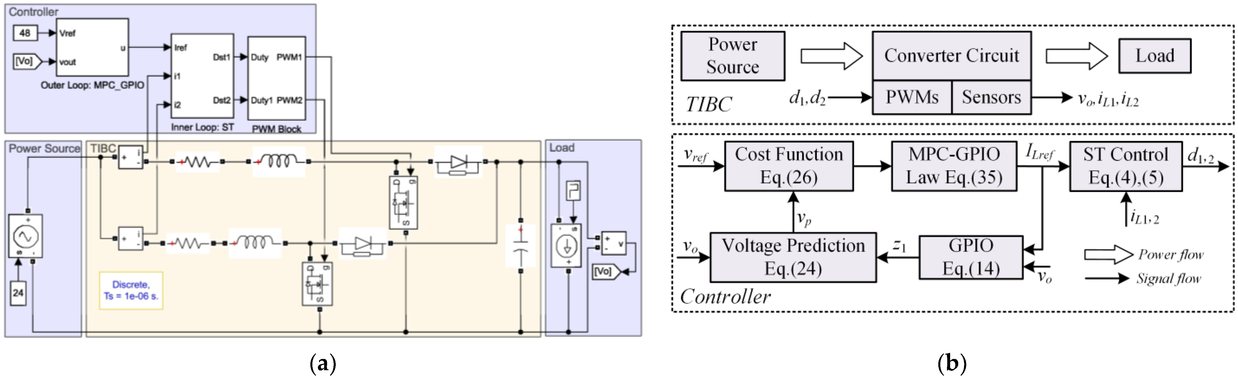
3.2.1. Design of GPIO

Unlikr the existing disturbance observer-based MPC studies [28,29], which assumed that the system disturbance is constant, the trend of the lumped disturbances is considered in this work. Following this idea, the GPIO introduced in [31] is constructed to estimate the time-varying uncertainties and disturbances.

The lumped disturbance $f$ and its first to N − 1-order derivatives are derived as the extended variables to the system in Equation (12) as

$$\left\{\begin{array}{c}\dot{\mathit{x}}=A\mathit{x}+Bu+Gh\left(t\right)\\ y=C\mathit{x} \end{array}\right.,$$

(13)

where $\mathit{x}={\left[v_o,f,f^{\left(1\right)},\dots ,f^{\left(n-1\right)}\right]}^T,h\left(t\right)$ is the N-order derivative of $f$. The matrices $A,B, \mathrm{and} G$ are as follows ($\mathit{E}$ is the identity matrix):

$$\begin{gathered} A_{\left(n+1\right)\times \left(n+1\right)}=\left[\begin{array}{cc}{\overline{A}}_{n\times 1}& {\mathit{E}}_{n\times n}\\ 0_{1\times 1}& {\mathbf{0}}_{1\times n}\end{array}\right],B_{\left(n+1\right)\times 1}=\left[\begin{array}{c}{b}_{\mathbf{0}\left(1\times 1\right)}\\ {\mathbf{0}}_{n\times 1}\end{array}\right],G_{\left(n+1\right)\times 1}=\left[\begin{array}{c}{\mathbf{0}}_{n\times 1}\\ 1_{1\times 1}\end{array}\right], \\ {C}_{1\times \left(n+1\right)}=\left[\begin{array}{cc}{1}_{1\times 1}& {\mathbf{0}}_{1\times n}\end{array}\right],{\overline{A}}_{\left(n+1\right)\times 1}=\left[\begin{array}{c}-a_{\mathbf{0}\left(1\times 1\right)}\\ {\mathbf{0}}_{n\times 1}\end{array}\right]. \end{gathered}$$

The original first-order system in Equation (12) is observable and controllable. Hence, it can be concluded that, for the extended system in Equation (13), $\left\{A,C\right\}$ is an observable pair.

Then, for the system in Equation (13), the GPIO is designed as follows:

$$\left\{\begin{array}{c}\dot{\widehat{\mathit{x}}}=A\widehat{\mathit{x}}+Bu+L\left(v_o-{\widehat{v}}_o\right)\\ \widehat{y}=C\widehat{\mathit{x}} \end{array}\right.,$$

(14)

where $\widehat{\mathit{x}}={\left[{\widehat{v}}_o,z_1,z_2,\dots ,z_{n-1}\right]}^T$ is the estimated state vector of $\mathit{x}$; the matrix $L$ is the gain vector of the observer to be designed, which has the following form:

$$L_{\left(n+1\right)\times 1}={\left[g_0,g_1,\dots ,g_n\right]}^T.$$

(15)

The estimation error vector of the GPIO is defined as

$$\mathit{e}=\mathit{x}-\widehat{\mathit{x}}.$$

(16)

Combining Equations (14) and (16), the error equation is

$$\dot{\mathit{e}}=A_e\mathit{e}+Gh\left(t\right),$$

(17)

where $A_e=A-LC$.

In practical applications, it is reasonable to suppose that $h\left(t\right)$ is bounded. Therefore, if the observer gain vector $L$ is properly selected to make the matrix $A_e$ a Hurwitz matrix, the error system in Equation (17) will be asymptotically stable.

In this paper, the characteristic polynomial of the matrix $A_e$ is

$$\lambda \left(s\right)=s^{n+1}+\left(g_0+a_0\right)s^n+{{\displaystyle \sum }}_{i=1}^n{g}_i{s}^{n-i}.$$

(18)

The pole placement method can be applied to tune the exact value of the gain vector $L$. To facilitate the design process of GPIO, referring to the bandwidth tuning method [26], all the poles of the error system in Equation (17) are placed at $-{\omega }_0$. Therefore, the characteristic polynomial of the matrix $A_e$ is rewritten as

$$\lambda \left(s\right)={\left(s+{\omega }_0\right)}^{n+1}.$$

(19)

Combining Equations (18) and (19), the gain vector $L$ is obtained as

$$g_0=C_{n+1}^1{\omega }_0-a_0,g_i=C_{n+1}^{i+1}{\omega }_0^{i+1},i=1,\dots ,n.$$

(20)

3.2.2. Design of MPC

The MPC can realize multiobjective optimization using the predefined cost function with weighing factors for different control objectives. The major ideas of MPC are summarized below.

• Prediction Model

The prediction model is utilized to predict the system outputs over several sampling periods, and it is generally constructed by the discrete form of Equation (12). As for the discretization methods, the Euler method and Taylor expansion are commonly used methods. For the Euler approximation-based MPC law, the computational effort raises sharply with the increase in the predictive horizon. The Taylor series expansion results in a continuous form prediction model, and the computational effort is independent of the prediction horizon. It also shows a smaller discretization error than the Euler approximation. Therefore, the Taylor series expansion is utilized in this work to formulate the prediction model.

Note that the voltage dynamics in Equation (12) is a first-order system; the future output voltage is predicted as

$$v_p\left(t+\tau \right)\approx v_o\left(t\right)+\tau {\dot{v}}_o\left(t\right)+\cdots +\frac{{\tau }^{\left(1+r\right)}}{\left(1+r\right)!}{v}_o{}^{\left(1+r\right)}\left(t\right),$$

(21)

where $v_p\left(t+\tau \right)$ is the predicted output voltage, and r is the control order, which defines the control input as an r-order derivative in the prediction time.

According to [32], a higher control order can increase the prediction accuracy and stability for higher-order nonlinear systems. To facilitate the analysis, the control order is chosen as one here, which is sufficient to ensure closed-loop stability. Then, the control sequence is defined as

$$\tilde{u}\left(t\right)={\left[u\left(t\right),\dot{u}\left(t\right)\right]}^T.$$

(22)

Combining the disturbance estimations given by GPIO, the derivatives of the output voltage are calculated as

$$\left\{\begin{array}{c}{\dot{v}}_o\left(t\right)=-a_0{v}_o\left(t\right)+b_{0}u\left(t\right)+z_1 \\ {\ddot{v}}_o\left(t\right)=a_0^2{v}_o\left(t\right)-a_0{b}_{0}u\left(t\right)+b_0\dot{u}\left(t\right)-a_0{z}_1+z_2\end{array}\right..$$

(23)

According to Equations (22) and (23), the output prediction in Equation (21) is rewritten as

$$v_p\left(t+\tau \right)=\left[{\Gamma }_v\left(\tau \right),{\Gamma }_u\left(\tau \right)\right]\left[\begin{array}{c}{Y}_1\left(t\right)\\ Y_2\left(t\right)\end{array}\right],$$

(24)

where ${\Gamma }_v\left(\tau \right)=1,{\Gamma }_u\left(\tau \right)=\left[\tau ,0.5{\tau }^2\right],Y_1\left(t\right)=v_o\left(t\right)$.

Furthermore,

$$Y_2\left(t\right)={\left[{\dot{v}}_o\left(t\right),{\ddot{v}}_o\left(t\right)\right]}^T=\tilde{Y}\left(t\right)+B_u\tilde{u}\left(t\right)+B_{z}z\left(t\right),$$

(25)

where

$$\tilde{Y}\left(t\right)={\left[-\widehat{a}{v}_o\left(t\right),{\widehat{a}}^2{v}_o\left(t\right)\right]}^T,B_u=\left[\begin{array}{cc}{b}_0& 0\\ -a_0{b}_0& b_0\end{array}\right],B_z=\left[\begin{array}{cc}1& 0\\ -a_0& 1\end{array}\right],z\left(t\right)={\left[z_1,z_2\right]}^T.$$

2.

Definition of Cost Function

The tracking error and control variations are selected as optimization objectives, and a generalized cost function is defined as

$$J=\frac{1}{2}\underset{0}{\overset{T_P}{{\displaystyle \int }}}\left[{[v_p\left(t+\tau \right)-v_r\left(t+\tau \right)]}^2+\rho u_c{\left(t\right)}^2\right]d\tau ,$$

(26)

where $v_r\left(t+\tau \right)$ is the reference value, $u_c\left(t\right)$ is the future control input, $T_P$ is the prediction time, and $\rho >0$ is the weighting factor.

In Equation (26), the first part penalizes the steady-state error of the converter, and the second part penalizes the control input variation. The purpose of MPC is to directly obtain the desired tracking performance by designing $T_s$ and $\rho$. The prediction time should be larger than the sampling time, and it determines the transient performance (fast or slow). On the other hand, a larger weighting factor $\rho$ means smaller control variation and voltage overshoot but decreases dynamic response.

3.

Optimized Control Law Design

The future control input $u_c\left(t\right)$ is determined by

$$u_c\left(t\right)={\Gamma }_r\left(\tau \right)\tilde{u}\left(t\right),$$

(27)

where ${\Gamma }_r\left(\tau \right)=\left[1,\tau \right]$.

The reference value for $Y_1\left(t\right),Y_2\left(t\right)$ is defined as $Y_{c1}\left(t\right),Y_{c2}\left(t\right)$; hence, the reference value $v_r\left(t+\tau \right)$ in Equation (26) can be expressed as

$$v_r\left(t+\tau \right)=\left[{\Gamma }_v\left(\tau \right),{\Gamma }_u\left(\tau \right)\right]\left[\begin{array}{c}{Y}_{c1}\left(t\right)\\ Y_{c2}\left(t\right)\end{array}\right].$$

(28)

For simplicity, omit the brackets $\left(·\right)$ for state variables. Then, according to Equations (24), (27), and (28), the cost function in Equation (26) is rewritten in the matrix form:

$$J=\frac{1}{2}\underset{0}{\overset{T_P}{{\displaystyle \int }}}\{{\{\left[{\Gamma }_v,{\Gamma }_u\right]\left[\begin{array}{c}{Y}_1-Y_{c1}\\ Y_2-Y_{c2}\end{array}\right]\}}^2+\rho {\left[{\Gamma }_r\tilde{u}\right]}^2\}d\tau .$$

(29)

Equation (29) can be expanded as

$$J=\frac{1}{2}\underset{0}{\overset{T_P}{{\displaystyle \int }}}\{\left[{\left(Y_1-Y_{c1}\right)}^T,{\left(Y_2-Y_{c2}\right)}^T\right]\left[\begin{array}{c}{\Gamma }_v^T\\ {\Gamma }_u^T\end{array}\right]\left[{\Gamma }_v,{\Gamma }_u\right]\left[\begin{array}{c}{Y}_1-Y_{c1}\\ Y_2-Y_{c2}\end{array}\right]+{\tilde{u}}^T{\Gamma }_r^T\rho {\Gamma }_r\tilde{u}\}d\tau .$$

(30)

Note that the integral variable $\tau$ only exists in ${\Gamma }_v,{\Gamma }_u,{\Gamma }_r$, Equation (30) can be further expressed as

$$\begin{gathered} J={\left(Y_1-Y_{c1}\right)}^T{\xi }_1\left(Y_1-Y_{c1}\right)+2{\left(Y_1-Y_{c1}\right)}^T{\xi }_2\left(Y_2-Y_{c2}\right) \\ +{\left(Y_2-Y_{c2}\right)}^T{\xi }_3\left(Y_2-Y_{c2}\right)+{\tilde{u}}^T{\xi }_4\tilde{u}, \end{gathered}$$

(31)

where

$$\begin{gathered} {\xi }_1=\frac{1}{2}{{\displaystyle \int }}_0^{T_P}{\Gamma }_v^T{\Gamma }_{v}d\tau =\frac{1}{2}{T}_P,{\xi }_2=\frac{1}{2}{{\displaystyle \int }}_0^{T_P}{\Gamma }_v^T{\Gamma }_{u}d\tau =\frac{1}{2}\left[\begin{array}{cc}\frac{T_P^2}{2}& \frac{T_P^3}{6}\end{array}\right], \\ {\xi }_3=\frac{1}{2}{{\displaystyle \int }}_0^{T_P}{\Gamma }_u^T{\Gamma }_{u}d\tau =\frac{1}{2}\left[\begin{array}{cc}\frac{T_P^3}{3}& \frac{T_P^4}{8}\\ \frac{T_P^4}{8}& \frac{T_P^5}{20}\end{array}\right],{\xi }_4=\frac{1}{2}{{\displaystyle \int }}_0^{T_P}{\Gamma }_r^T\rho {\Gamma }_{r}d\tau =\frac{\rho }{2}\left[\begin{array}{cc}{T}_P& \frac{T_P^2}{2}\\ \frac{T_P^2}{2}& \frac{T_P^3}{3}\end{array}\right]. \end{gathered}$$

The part of Equation (31) related to $\tilde{u}\left(t\right)$ is

$$\begin{gathered} J\left(\tilde{u}\right)={\tilde{u}}^T{B}_u^T{\xi }_3{B}_u\tilde{u}+{\tilde{u}}^T{\xi }_4\tilde{u}+2{\left(Y_1-Y_{c1}\right)}^T{\xi }_2{B}_u\tilde{u} \\ +2{\left[\tilde{Y}\left(t\right)+B_{z}z\left(t\right)\right]}^T{\xi }_3{B}_u\tilde{u}-2Y_{c2}^T{\xi }_3{B}_u\tilde{u}. \end{gathered}$$

(32)

The derivative of $J\left(\tilde{u}\right)$ to $J\left(\tilde{u}\right)$ is

$$\frac{\partial J\left(\tilde{u}\right)}{\partial \tilde{u}}=2\left(B_u^T{\xi }_3{B}_u+{\xi }_4\right)\tilde{u}+2B_u^T{\xi }_2^T\left(Y_1-Y_{c1}\right)+2B_u^T{\xi }_3^T\left[\tilde{Y}\left(t\right)+B_{z}z\left(t\right)-Y_{c2}\right].$$

(33)

With $\partial J\left(\tilde{u}\right)/\partial \tilde{u}=0$, the optimal control law from Equation (26) is

$${\tilde{u}}^{*}\left(t\right)=-{\left(B_u^T{\xi }_3{B}_u+{\xi }_4\right)}^{-1}{B}_u^T\left\{{\xi }_2^T\left(Y_1-Y_{c1}\right)+B_a^{-1}\left[\tilde{Y}\left(t\right)+B_{z}z\left(t\right)-Y_{c2}\right]\right\}.$$

(34)

Taking the first row of ${\tilde{u}}^{*}\left(t\right)$, we get

$$u\left(t\right)=-k_1\left(v_o-v_{ref}\right)+\frac{{\dot{v}}_r+a_0{v}_o-z_1}{b_0},$$

(35)

where $k_1$ is the first row of the matrix ${\left(B_u^T{\xi }_3{B}_u+{\xi }_4\right)}^{-1}{B}_u^T{\xi }_2^T$.

$$k_1=\frac{4T_P{b}_0\left[33b_0^2{T}_P^2+40\rho a_0{T}_P+180\rho \right]}{\left(3b_0^4+48\rho a_0{b}_0^2\right)T_P^4+96\rho a_0{b}_0^2{T}_P^3+104\rho b_0^2{T}_P^2+240{\rho }^2}.$$

3.2.3. Stability Analysis

Stability is an essential property for a closed-loop control system and must be guaranteed. A strict analysis is provided here to show the convergence characteristic of the proposed MPC-GPIO method.

With the tracking error as $e_v=v_o-v_r$, Equation (35) is substituted into Equation (12), and the error dynamics of the MPC law can be written as

$${\dot{e}}_v=-b_0{k}_1{e}_v+f-z_1.$$

(36)

If there are no disturbances, the tracking error follows ${\dot{e}}_v=-b_0{k}_1{e}_v$, and the closed-loop system is asymptotically stable.

In the presence of disturbances, for simplicity, the second-order GPIO is selected in this section. The estimation error is defined as $e_s=v_o-{\widehat{v}}_o,$ $e_1=f-z_1$, $e_2=f^{\left(1\right)}-z_2$. Then, the error dynamics of the control system is

$${\dot{E}}_{v,r}=A_{\epsilon }{E}_{v,r}+B_{\epsilon }h\left(t\right),$$

(37)

where $E_{v,r}={\left[e_v, e_s,e_1,e_2\right]}^T,B_{\epsilon }={\left[0,0,0,-1\right]}^T,A_{\epsilon }=\left[\begin{array}{cc}-b_0{k}_1& H_{\left(1\times 3\right)}\\ {\mathbf{0}}_{3\times 1}& A_{e\left(3\times 3\right)}\end{array}\right],H=\left[\begin{array}{ccc}0& 1& 0\end{array}\right]$.

Suppose that the second-order derivative of lumped disturbance $h\left(t\right)$ is bounded. According to Equations (18)–(20), the eigenvalues of matrix $A_{\epsilon }$ in Equation (37) are

$${\lambda }_1=-b_0{k}_1,{\lambda }_2={\lambda }_3={\lambda }_4=-{\omega }_0.$$

(38)

Therefore, the matrix $A_{\epsilon }$ is Hurwitz-stable, and the voltage control loop is asymptotically stable.

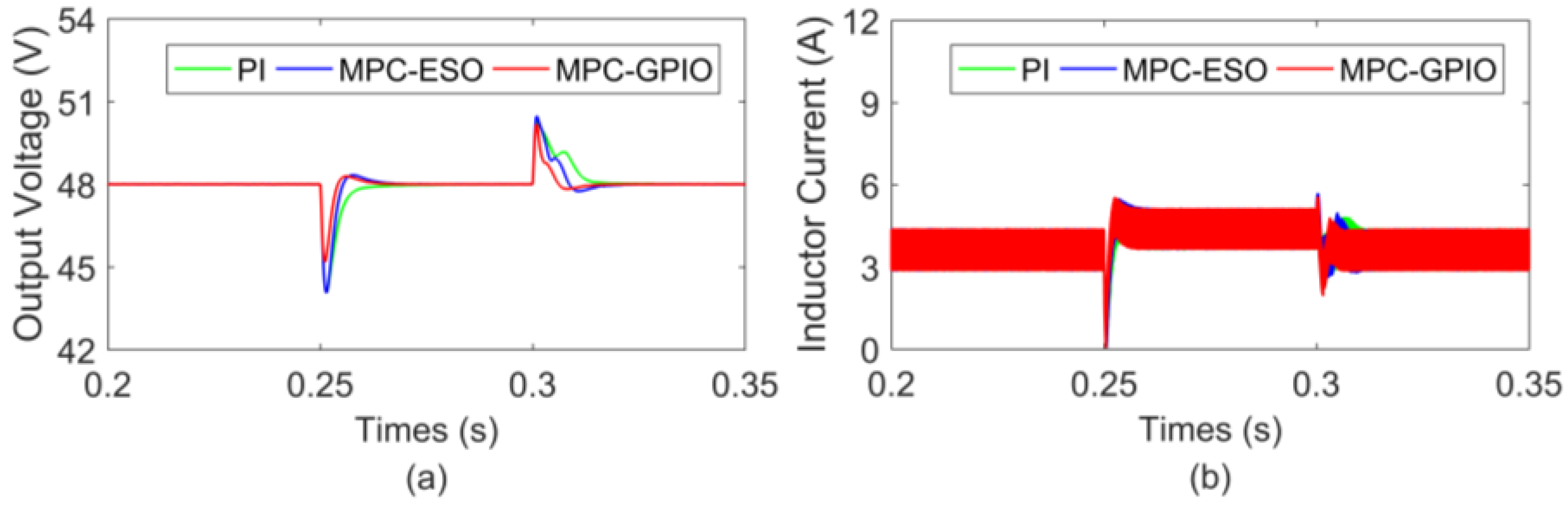
4. Simulation Results

The converter circuit with the proposed MPC-GPIO control strategy was established in MATLAB/Simulink, as shown in Figure 3a, and the block diagram of the simulation is shown in Figure 3b. The detailed circuit parameters are given in

Table 1. Detailed parameters of the converter.

Parameter	Symbol	Value
Nominal input voltage	$V_{in}$	16–24 V
Nominal output voltage	$V_o$	48 V
Nominal inductance	$L_{1,2}$	200 μH
Nominal capacitance	$C$	400 μF
Load power	$P_{rate}$	300 W
Switching frequency	$f_s$	50 kHz

. For comparison, the typical cascaded-loop PI method and the extended state observer-based MPC method (MPC-ESO) proposed in [28] are also developed in this section. The MPC-GPIO and MPC-ESO method are tuned with the same control parameters, given as $T_P=4ms,\rho =4,{\omega }_0=500$. Furthermore, both the MPC-GPIO and the MPC-ESO methods utilize the ST algorithm in Equation (5) as the current controller, which is tuned as $\alpha =0.05,\beta =30$. For the cascaded-loop PI controller, the bandwidth tuning method is utilized, and the current loop is tuned as $k_p=0.05,k_i=30$, while the voltage loop is tuned as $k_p=0.5,k_i=80$.

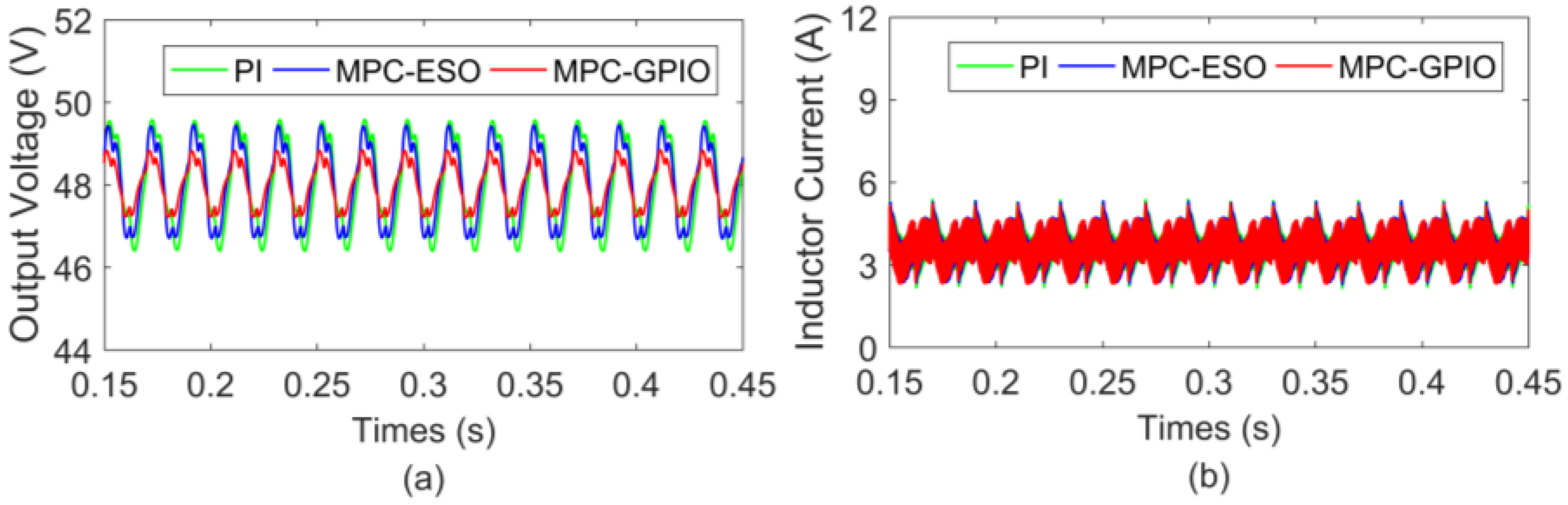
4.1. Circuit Parameter Uncertainties

For power converters, the value of circuit parameters may change due to long-term use. Moreover, the parasitic parameters of some key components will also change and affect the control performance. Hence, several typical cases are tested, including the variation in inductance, capacitance, and parasitic resistance.

Figure 4 shows the dynamic responses of TIBC under different cases, where the given value changes from 48 V to 56 V at 0.3 s. According to Figure 4a,b, when the nominal inductance or capacitance deviates 20% from the rated value, the proposed MPC-GPIO method shows almost the same voltage response curves. As shown in Figure 4c, the change in inductor parasitic resistance also has no significant influence on the control performance, and the voltage overshoot is reduced when there is a large inductor parasitic resistance. As shown in Figure 4d, the dynamic response curves overlap when the capacitor parasitic resistance changes. Therefore, the proposed MPC-GPIO method is robust to parameter uncertainties.

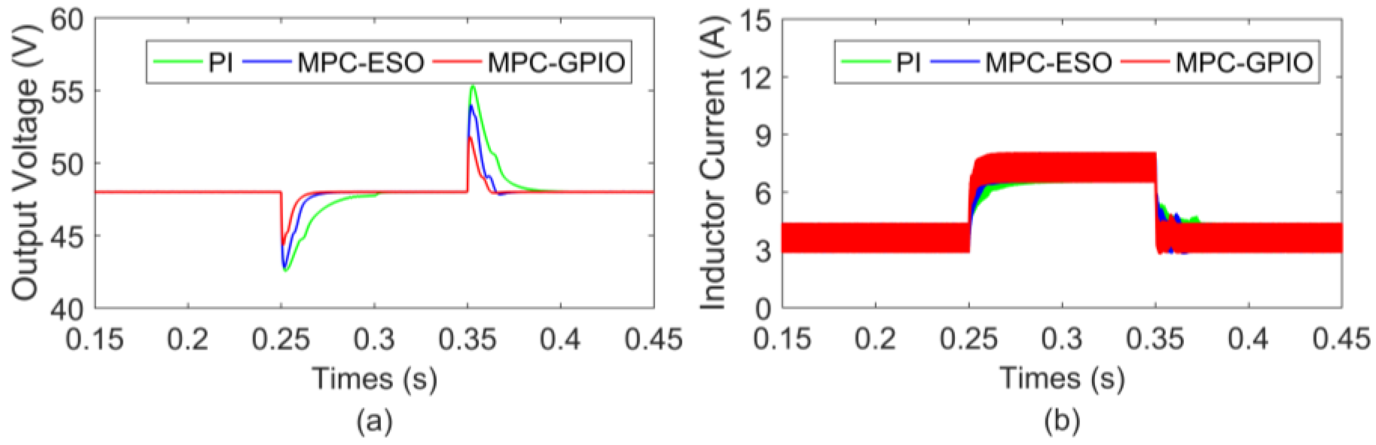
4.2. Power Source Disturbances

The robustness of the MPC-GPIO method against power source disturbance is tested in this section.

First, the input voltage decreases from 24 V to 20 V at 0.25 s; then, the input voltage increases to 24 V at 0.3 s. The load resistance is set as 13.7 Ω. The dynamic response curves of the converter are shown in Figure 5. As can be seen, all three controllers can eliminate the output error resulting from the input voltage variations. However, the cascaded PI method shows a long recovery time. The MPC-ESO method has fast convergence characteristics, but it still has larger voltage decreases/increases than the proposed MPC-GPIO method.

Then, the time-varying disturbance is applied to TIBC, and the input voltage is set to $V_{in}=24+2\sin \left(100\pi t\right)V$. The corresponding response curves of the converter are shown in Figure 6. As can be observed, the cascaded PI method and MPC-ESO method result in a large voltage perturbation. The voltage perturbation of the MPC-GPIO method is significantly reduced. Therefore, the MPC-GPIO controller exhibits stronger robustness against power source disturbances.

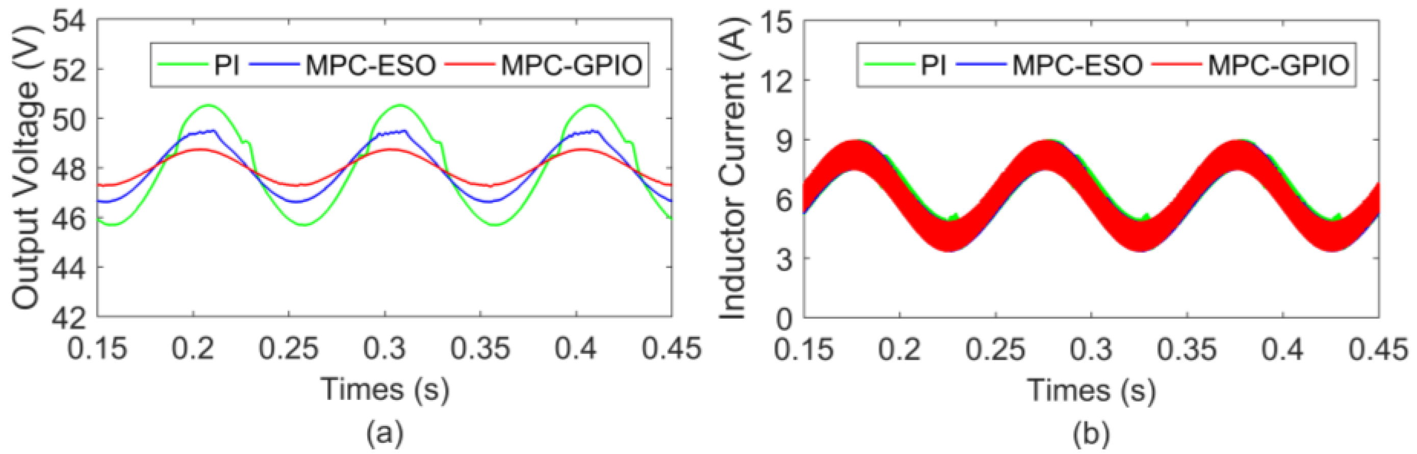
4.3. Load Disturbances

The load disturbance is applied to the converter in this section. First, the input voltage is set as 24 V; the load resistance decreases from 13.7 Ω to 6.85 Ω at 0.25 s and increases from 6.85 Ω to 13.7 Ω at 0.35 s. The dynamic response curves of TIBC are shown in Figure 7. As can be seen, the voltage perturbations and recovery time of the three controllers are different in the transient process. However, compared with the other two controllers, the proposed MPC-GPIO controller shows a smaller voltage perturbation and faster dynamic response.

Furthermore, the time-varying load current is also applied to the converter, and the results are shown in Figure 8. A controlled current source is employed as the power load, set as $i_o=6+2\sin \left(20\pi t\right)A$. When the load current changes, the output voltage changes sinusoidally. Compared with the other two controllers, the proposed MPC-GPIO controller still has a better control effect.

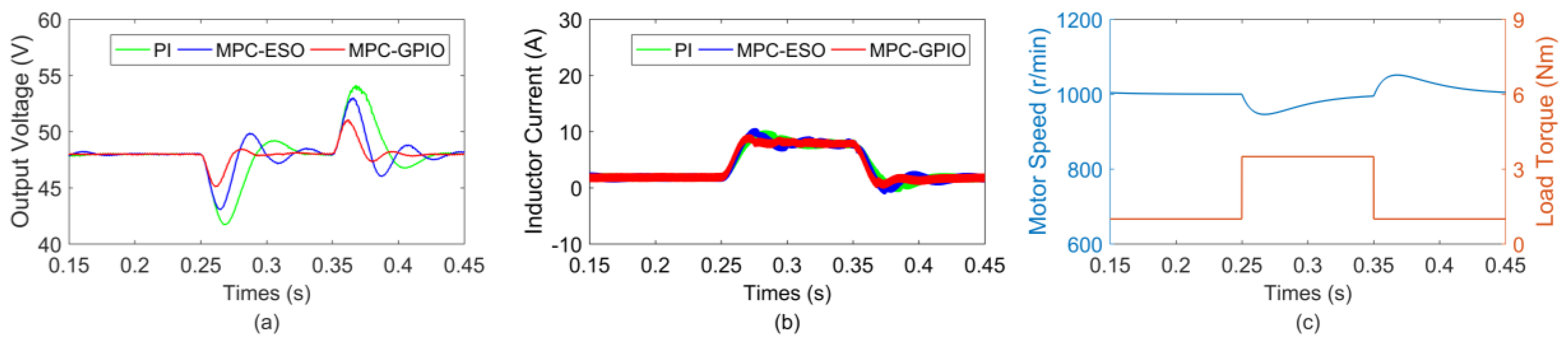
4.4. Electric Machine Load

The electric machine load was applied to the converter, and the simulation results are shown in Figure 9. The permanent magnet synchronous machine, voltage-source inverter, and SVPWM were established in MATLAB/Simulink. For the motor, the stator resistance was 0.108 Ω, the d–q axis inductance was 2.4 mH, and the rotor flux was 0.045 Wb. The reference motor speed was set as 1000 r/min, and the load torque in the initial state was 1 N·m. At 0.25 s, the load torque stepped to 3.5 N·m and stepped back to 1 N·m at 0.35 s.

As can be observed from Figure 9, when the load torque changes, the output voltage deviates from the nominal value and generates a certain oscillation. For the cascaded PI method, there is large voltage perturbation, and the recovery time is nearly 0.75 s. For the MPC-ESO method, the voltage perturbation is reduced but the recovery time is longer. For the proposed MPC-GPIO method, both the voltage perturbation and the recovery time are reduced significantly. Therefore, the proposed method has a better control effect.

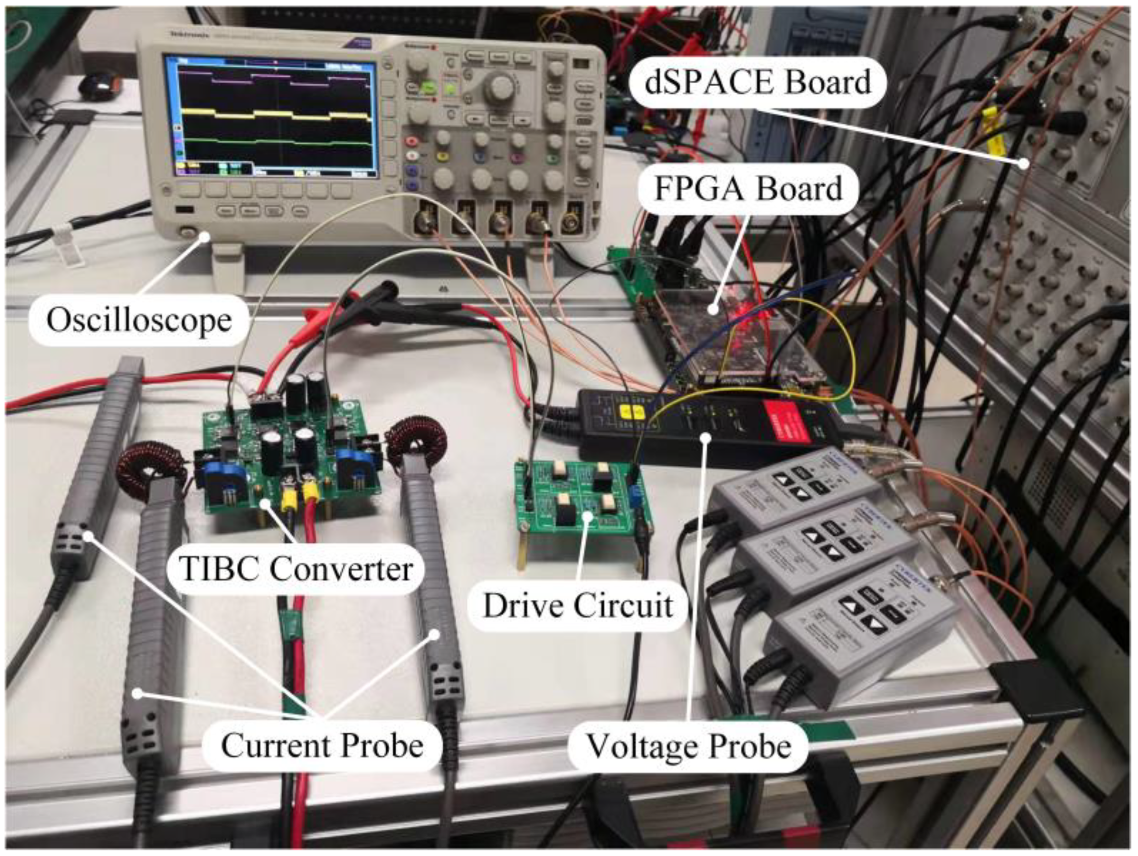
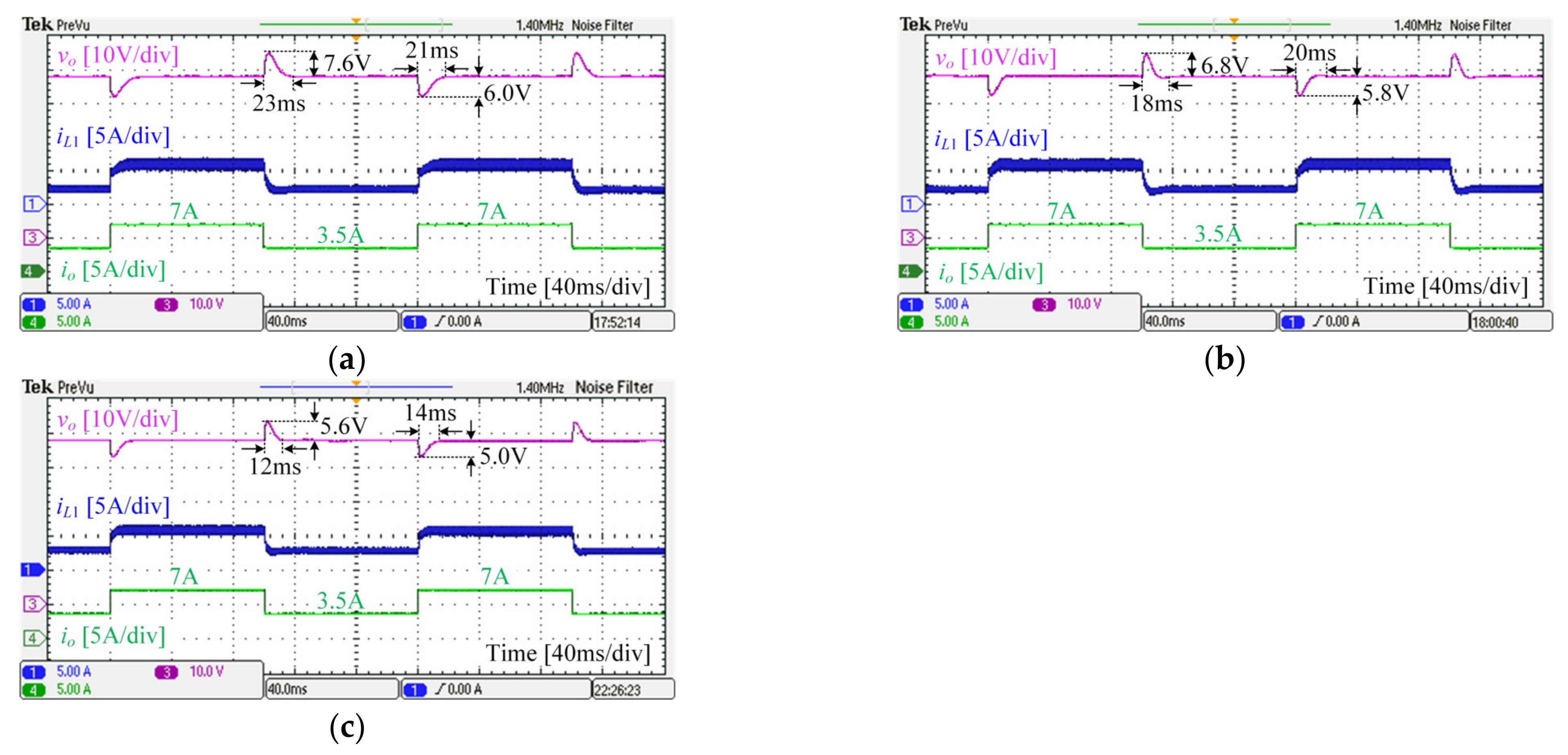
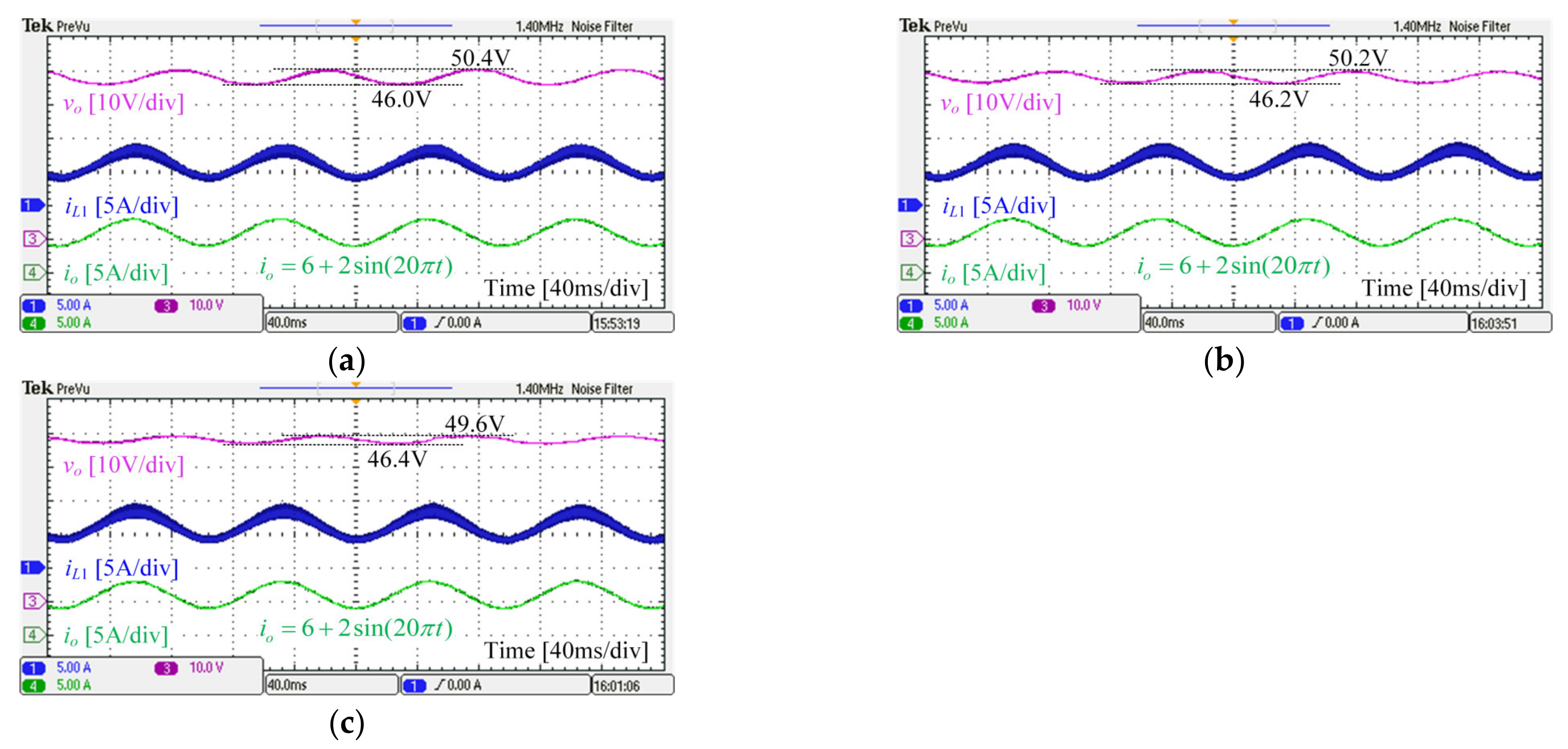
5. Experimental Results

An experimental setup is constructed and experimental tests are conducted in this secyion to demonstrate the superiority of the MPC-GPIO method, as shown in Figure 10. The converter circuit parameters are given in Table 1, and the detailed laboratory instruments used in the experiment are listed in

Table 2. Detailed instruments in the experiment.

Laboratory Instruments	Marking	Quantity
dSPACE board	DS1007	1
Power source	PEL-80/40.5	1
Electric load	NHR 4760	1
FPGA board	Altea EP4CE15F23C8	1
Voltage sensor	Cybertek DP6150A	1
Current sensor	Cybertek CP8050A	3
Oscilloscope	Tektronix DPO2014B	1

. Furthermore, the measurement accuracy for the voltage sensor and current sensor are ±2% and ±1%, respectively.

The algorithm is realized in the dSPACE board, and then the control signals are sent to FPGA to realize the phase shift. The typical cascaded-loop PI algorithm and the MPC-ESO controller are chosen as the benchmarks. The parameters of MPC-GPIO and MPC-ESO are tuned as $T_P=4ms,\rho =4,{\omega }_0=500$, and the ST algorithm in the current loop is tuned as $\alpha =0.05,\beta =30$. For the cascaded-loop PI controller, the current loop is tuned as $k_p=0.05,k_i=30$, and the voltage loop is tuned as $k_p=0.5,k_i=80$.

5.1. Step Load Disturbance

The step load disturbance was adopted, and the step load current between 3.5 A and 7 A was applied to TIBC periodically using the programmable electronic load. The corresponding experimental results of the cascaded PI controller, MPC-ESO controller, and MPC-GPIO controllers are shown in Figure 11.

According to Figure 11, when the load current changed periodically, all three controllers could regulate the output voltage to the given value of 48 V. However, at the moment of disturbances, the cascaded-loop PI controller exhibited the largest voltage perturbations and longest recovery time, and the MPC-GPIO controller showed the best voltage regulation performance.

5.2. Time-Varying Load Disturbance

To demonstrate the superiority of the MPC-GPIO method in dealing with time-varying disturbance, the sinusoidal form load current was applied to the converter, as $i_o=6+2\sin \left(20\pi t\right)A$. Figure 12 shows the experimental results of TIBC under three controllers.

It can be observed from Figure 12 that, when the load current varies, the output voltage also changes periodically. For the cascaded PI controller, the output voltage ranged from 46 V to 50.4 V. For the MPC-ESO controller, the output voltage ranged from 46.2 V to 50.2 V. The proposed MPC-GPIO controller had the strongest robustness, and its output voltage ranged from 46.4 V to 49.6 V.

6. Conclusions

To overcome the nonminimum phase behaviors and nonlinearity of the boost converter, a novel offset-free continuous control set model predictive controller was developed in this study. Based on the dual-loop control framework, the ST control was adopted to the current loop, and the equivalent control plant was obtained through the linearization technique. The disturbance estimation method was utilized, and all the system uncertainties were considered as the lumped disturbance. To remove the offset within MPC, a generalized proportional integral observer was designed to compensate for the predictive model online. Considering the steady-state error and control input variation, an optimization problem was constructed and solved offline; thus, an explicit optimal control law was obtained.

To verify the effectiveness of the proposed controller, simulation and experimental tests were carried out under different cases. Compared with the cascaded PI controller and the MPC-ESO controller, the voltage regulation performance of the proposed MPC-GPIO controller was improved significantly.

References

1. Mesquita da Silva, J.A.; Deaecto, G.S.; Barros, T.A.d.S. Analysis and Design Aspects of Min-Type Switching Control Strategies for Synchronous Buck–Boost Converter. Energies 2022, 15, 2302. [Google Scholar] [CrossRef]
2. Fantino, R.A.; Christian, S.F.; Balda, J.C. Synchronous-Variable-Frequency Control of Bidirectional DCM Interleaved DC–DC Converter for Wide-Range Enhanced Efficiency. IEEE Trans. Ind. Electron. 2021, 69, 5844–5853. [Google Scholar] [CrossRef]
3. Rahimi, T.; Ding, L.; Kheshti, M.; Faraji, R. A ZVS Three-Phase Interleaved DC-DC converter with SFM control method for the Microgrid Applications. In Proceedings of the 2020 11th Power Electronics, Drive Systems, and Technologies Conference (PEDSTC), Tehran, Iran, 4–6 February 2020; pp. 1–5. [Google Scholar] [CrossRef]
4. Kabalo, M.; Paire, D.; Blunier, B.; Bouquain, D.; Simões, M.G.; Miraoui, A. Experimental evaluation of four-phase floating interleaved boost converter design and control for fuel cell applications. IET Power Electron. 2013, 6, 215–226. [Google Scholar] [CrossRef] [Green Version]
5. Garcia, F.S.; Pomilio, J.A.; Spiazzi, G. Modeling and Control Design of the Interleaved Double Dual Boost Converter. IEEE Trans. Ind. Electron. 2012, 60, 3283–3290. [Google Scholar] [CrossRef]
6. El Beid, S.; Doubabi, S. DSP-Based Implementation of Fuzzy Output Tracking Control for a Boost Converter. IEEE Trans. Ind. Electron. 2013, 61, 196–209. [Google Scholar] [CrossRef]
7. Kobaku, T.; Patwardhan, S.C.; Agarwal, V. Experimental Evaluation of Internal Model Control Scheme on a DC–DC Boost Converter Exhibiting Nonminimum Phase Behavior. IEEE Trans. Power Electron. 2017, 32, 8880–8891. [Google Scholar] [CrossRef]
8. Xu, Q.; Jiang, W.; Blaabjerg, F.; Zhang, C.; Zhang, X.; Fernando, T. Backstepping Control for Large Signal Stability of High Boost Ratio Interleaved Converter Interfaced DC Microgrids With Constant Power Loads. IEEE Trans. Power Electron. 2019, 35, 5397–5407. [Google Scholar] [CrossRef]
9. Yuan, C.; Bai, H.; Ma, R.; Huangfu, Y. Large-Signal Stability Analysis and Design of Finite-Time Controller for the Electric Vehicle DC Power System. IEEE Trans. Ind. Appl. 2021, 58, 868–878. [Google Scholar] [CrossRef]
10. Yang, T.; Liao, Y. Discrete Sliding Mode Control Strategy for Start-Up and Steady-State of Boost Converter. Energies 2019, 12, 2990. [Google Scholar] [CrossRef]
11. Li, X.; Chen, X. A Multi-Index Feedback Linearization Control for a Buck-Boost Converter. Energies 2021, 14, 1496. [Google Scholar] [CrossRef]
12. You, J.; Fan, W.; Yu, L.; Fu, B.; Liao, M. Disturbance Rejection Control Method of Double-Switch Buck-Boost Converter Using Combined Control Strategy. Energies 2019, 12, 278. [Google Scholar] [CrossRef] [Green Version]
13. Valencia-Rivera, G.H.; Amaya, I.; Cruz-Duarte, J.M.; Ortíz-Bayliss, J.C.; Avina-Cervantes, J.G. Hybrid Controller Based on LQR Applied to Interleaved Boost Converter and Microgrids under Power Quality Events. Energies 2021, 14, 6909. [Google Scholar] [CrossRef]
14. Guo, K.; Liu, Q.; Xi, X.; Mao, M.; Wan, Y.; Wu, H. Coordinated Control Strategy of a Combined Converter in a Photovoltaic DC Boost Collection System under Partial Shading Conditions. Energies 2020, 13, 474. [Google Scholar] [CrossRef] [Green Version]
15. Barhoumi, E.M.; Ben Belgacem, I.; Khiareddine, A.; Zghaibeh, M.; Tlili, I. A Neural Network-Based Four Phases Interleaved Boost Converter for Fuel Cell System Applications. Energies 2018, 11, 3423. [Google Scholar] [CrossRef] [Green Version]
16. Xu, Q.; Yan, Y.; Zhang, C.; Dragicevic, T.; Blaabjerg, F. An Offset-Free Composite Model Predictive Control Strategy for DC/DC Buck Converter Feeding Constant Power Loads. IEEE Trans. Power Electron. 2019, 35, 5331–5342. [Google Scholar] [CrossRef]
17. Ebad, M.; Song, B.-M. Accurate model predictive control of bidirectional DC-DC converters for DC distributed power systems. In Proceedings of the 2012 IEEE Power and Energy Society General Meeting, San Diego, CA, USA, 22–26 July 2012; pp. 1–8. [Google Scholar] [CrossRef]
18. Vazquez, S.; Rodriguez, J.; Rivera, M.; Franquelo, L.G.; Norambuena, M. Model Predictive Control for Power Converters and Drives: Advances and Trends. IEEE Trans. Ind. Electron. 2017, 64, 935–947. [Google Scholar] [CrossRef] [Green Version]
19. Kim, S.-K.; Park, C.R.; Kim, J.-S.; Lee, Y.I. A Stabilizing Model Predictive Controller for Voltage Regulation of a DC/DC Boost Converter. IEEE Trans. Control. Syst. Technol. 2014, 22, 2016–2023. [Google Scholar] [CrossRef]
20. Zhang, H.; Li, Y.; Xie, R.; Song, J.; Liang, B.; Huangfu, Y. Adaptive Model Predictive Control of an Interleaved Boost Converter Using Real-Time Updated Model. IEEE Trans. Power Electron. 2022, 38, 1720–1731. [Google Scholar] [CrossRef]
21. Ramirez, R.O.; Espinoza, J.R.; Baier, C.R.; Rivera, M.; Villarroel, F.; Guzman, J.I.; Melin, P.E. Finite-State Model Predictive Control With Integral Action Applied to a Single-Phase Z-Source Inverter. IEEE J. Emerg. Sel. Top. Power Electron. 2018, 7, 228–239. [Google Scholar] [CrossRef]
22. Favato, A.; Carlet, P.G.; Toso, F.; Torchio, R.; Bolognani, S. Integral Model Predictive Current Control for Synchronous Motor Drives. IEEE Trans. Power Electron. 2021, 36, 13293–13303. [Google Scholar] [CrossRef]
23. Yang, J.; Zheng, W.X.; Li, S.; Wu, B.; Cheng, M. Design of a Prediction-Accuracy-Enhanced Continuous-Time MPC for Disturbed Systems via a Disturbance Observer. IEEE Trans. Ind. Electron. 2015, 62, 5807–5816. [Google Scholar] [CrossRef]
24. He, L.; Wang, F.; Ke, D. FPGA-Based Sliding-Mode Predictive Control for PMSM Speed Regulation System Using an Adaptive Ultralocal Model. IEEE Trans. Power Electron. 2021, 36, 5784–5793. [Google Scholar] [CrossRef]
25. Izci, D.; Ekinci, S. A novel improved version of hunger games search algorithm for function optimization and efficient controller design of buck converter system. E-Prime-Adv. Electr. Eng. Electron. Energy 2022, 2, 100039. [Google Scholar] [CrossRef]
26. Xiong, W.; Wang, Z.; Zhang, B.; Li, S. Robust Voltage Regulation for DC–DC Converters via a Predictive GPIO-Based Control Approach. IEEE Trans. Circuits Syst. II Express Briefs 2022, 69, 4864–4868. [Google Scholar] [CrossRef]
27. Zhou, L.; Eull, M.; Preindl, M. Optimization-Based Estimation and Model Predictive Control for High Performance, Low Cost Software-Defined Power Electronics. IEEE Trans. Power Electron. 2022, 38, 1022–1035. [Google Scholar] [CrossRef]
28. Liu, H.; Li, S. Speed Control for PMSM Servo System Using Predictive Functional Control and Extended State Observer. IEEE Trans. Ind. Electron. 2011, 59, 1171–1183. [Google Scholar] [CrossRef]
29. Po, L.; Ruiyu, L.; Tianying, S.; Jingrui, Z.; Zheng, F. Composite adaptive model predictive control for DC–DC boost converters. IET Power Electron. 2018, 11, 1706–1717. [Google Scholar] [CrossRef]
30. Zhang, H.; Ma, R.; Han, C.; Xie, R.; Liang, B.; Li, Y. Advanced Control Design of Interleaved Boost Converter for Fuel Cell Applications. In Proceedings of the IECON 2020 The 46th Annual Conference of the IEEE Industrial Electronics Society, Singapore, 18–21 October 2020; pp. 5000–5005. [Google Scholar] [CrossRef]
31. Chen, W.-H.; Yang, J.; Guo, L.; Li, S. Disturbance-Observer-Based Control and Related Methods—An Overview. IEEE Trans. Ind. Electron. 2015, 63, 1083–1095. [Google Scholar] [CrossRef] [Green Version]
32. Chen, W.-H.; Ballance, D.J.; Gawthrop, P.J. Optimal control of nonlinear systems: A predictive control approach. Automatica 2003, 39, 633–641. [Google Scholar] [CrossRef]
Figure 1. The topology of TIBC.
Energies 16 01245 g001
Figure 2. The cascaded dual-loop control structure.
Energies 16 01245 g002
Figure 3. Snapshot and block diagram of the simulation: (a) simulation of TIBC under MATLAB/Simulink; (b) block diagram of simulation.
Energies 16 01245 g003
Figure 4. Dynamic response of converter under parameter uncertainties: (a) the variation of inductance; (b) the variation of capacitance; (c) the variation of parasitic resistance of the inductor; (d) the variation of parasitic resistance of the capacitor.
Energies 16 01245 g004
Figure 5. Dynamic response of TIBC under step input voltage change at 0.25 s and 0.3 s: (a) output voltage; (b) inductor current.
Energies 16 01245 g005
Figure 6. Dynamic response of TIBC with the input voltage, V i n = 24 + 2 sin 100 π t V : (a) output voltage; (b) inductor current.
Energies 16 01245 g006
Figure 7. Dynamic response of TIBC under step load disturbance at 0.25 s and 0.3 s: (a) output voltage; (b) inductor current.
Energies 16 01245 g007
Figure 8. Dynamic response of TIBC with the load current is set as i o = 6 + 2 sin 20 π t A : (a) output voltage; (b) inductor current.
Energies 16 01245 g008
Figure 9. Dynamic response of converter with electric machine load: (a) output voltage; (b) inductor current; (c) motor speed and load torque.
Energies 16 01245 g009
Figure 10. Experimental platform.
Energies 16 01245 g010
Figure 11. Experimental results of different controllers under step load current changes: (a) cascaded PI controller; (b) MPC-ESO controller; (c) MPC-GPIO controller.
Energies 16 01245 g011
Figure 12. Experimental results of different controllers under sinusoidal load disturbance: (a) cascaded PI controller; (b) MPC-ESO controller; (c) MPC-GPIO controller.
Energies 16 01245 g012