Review

Overview of Numerical Simulation of Solid-State Anaerobic Digestion Considering Hydrodynamic Behaviors, Phenomena of Transfer, Biochemical Kinetics and Statistical Approaches

1
TIMR (Integrated Transformations of Renewable Matter), Université de Technologie de Compiègne, ESCOM, Centre de Recherches Royallieu, 60203 Compiègne, France
2
GéoLab, Institut Polytechnique UniLaSalle, Rue Pierre Waguet, 60026 Beauvais, France
3
Institut Polytechnique UniLaSalle, Université d’Artois, ULR 7519, Rue Pierre Waguet, 60026 Beauvais, France
*
Authors to whom correspondence should be addressed.
Energies 2023, 16(3), 1108; https://doi.org/10.3390/en16031108
Submission received: 10 December 2022 / Revised: 8 January 2023 / Accepted: 17 January 2023 / Published: 19 January 2023

Abstract

:
Anaerobic digestion (AD) is a promising way to produce renewable energy. The solid-state anaerobic digestion (SSAD) with a dry matter content more than 15% in the reactors is seeing its increasing potential in biogas plant deployment. The relevant processes involve multiple of evolving chemical and physical phenomena that are not crucial to conventional liquid-state anaerobic digestion processes (LSAD). A good simulation of SSAD is of great importance to better control and operate the reactors. The modeling of SSAD reactors could be realized either by theoretical or statistical approaches. Both have been studied to a certain extent but are still not sound. This paper introduces the existing mathematical tools for SSAD simulation using theoretical, empirical and advanced statistical approaches and gives a critical review on each type of model. The issues of parameter identifiability, preference of modeling approaches, multiscale simulations, sensibility analysis, particularity of SSAD operations and global lack of knowledge in SSAD media evolution were discussed. The authors call for a stronger collaboration of multidisciplinary research in order to further developing the numeric simulation tools for SSAD.

1. Introduction

1.1. Anaerobic Digestion for Biogas Production

Anaerobic digestion (AD) is one of the promising solutions for recovering the energy contained in various organic wastes. Inputs to anaerobic digestion can be agricultural by-products, industrial effluents, sludge from wastewater treatment plants (WWTP) and the biodegradable fraction of household waste [1]. Depending on the dry matter content (DM) operated in digestors, there are two other types of technology: liquid-state AD (DM < 15%) and solid-state AD (DM > 15%) [2].
Liquid-state AD (LSAD), also called wet anaerobic digestion, is the technology conventionally employed by the industry. It is adapted to substrates with a relatively high water content (e.g., sewage sludge). On one hand, its humid character allows a more efficient homogenization of the mixture. On the other hand, it dilutes substrates to keep the DM level relatively low and stable in the reactors. At the end of the digestion, phase separation of digestate is generally required to (1) maintain the biomass concentration in the reactors by recirculation of its liquid phase and (2) concentrate the digestate for further agricultural usage. It should be noted that LSAD technology shows a high level of maturity. Around 90% of the AD reactors in France run in LSAD mode [3]. The disadvantage of LSAD lies on the fact of its low organic loading leading to low biogas yield rate and the high energy and financial costs for digestate phase separation and downstream treatment.

1.2. Solid-State Anaerobic Digestion

Although currently it does not represent a large market share, the solid-state anaerobic digestion (SSAD), also called dry anaerobic digestion, is being increasingly adopted in newly built biogas plant projects [4]. The interest of SSAD is based on the fact that it operates with a higher organic loading that gives rise to more robust biochemical reactions. Moreover, it requires less water for the dilution of the substrates upstream and consequently, less phase separation downstream. As the medium is more concentrated, solid-state digesters require less volume and less heating compared to LSAD reactors. These advantage of SSAD makes possible the construction of a low-cost biogas plant. It is also acknowledged that SSAD reactors can tolerate a relatively higher organic loading [5]. Nevertheless, the disadvantages of this type of technology are also obvious. It is less suitable for processing liquid substrates. Its solid character makes agitation very difficult, resulting in less contact between the substrates and the microorganisms. In addition, incomplete homogenization can lead to a local concentration of inhibiting compounds (e.g., ammonia, volatile fatty acids—VFA) that limit or even stop the methanogenic microbial activities [6]. Solid-state digestion, therefore, requires more sophisticated equipment (pumps, agitators, heat exchangers, etc.) for implementation. The maturity of solid-state anaerobic digestion is currently less marked than that of the LSAD process.
SSAD can be realized by various processes. Many review papers like Fagbohungbe et al. (2014) [7], Kothari et al. (2014) [8], Xu et al. (2015) [9], André et al. (2018) [3] and Franca and Bassin (2020) [10] have given comprehensive overview of various SSAD reactors available at different scales. To be general, we can find the continuous processes with the recirculation of liquid digestate or biogas serving as stirring methods of the solid media. Compared to continuous processes, batch reactors with discontinuous operation are more common in SSAD [11], like container-type and garage-type digesters. One has to note that the DM content is not a determining factor defining LSAD or SSAD. The solid behavior could be seen with DM content less than 15% for reactors charged by cereal straw. Media of DM content more than 15% but with sewage sludge can be pasty, an intermediary state between LSAD and SSAD.
In all cases, different from LSAD reactors, three phases are generally present in SSAD reactors: a relatively immobilized solid phase representing the bulk of solid substrates pending degradation, a liquid phase resulting from the inoculum (the leachate as well as the percolate across the solid bulk) and finally a gas phase rich in biogas found in the headspace of reactors and the pores in solid bulk (due to its characteristics similar to porous media). Depending on the technology used, the solid phases could be partially immerged in the liquid phase which is the collected at the bottom of reactors, heated through a heat exchanger and regularly sprayed to the top of bulk for a new round of percolation. This recirculation allows to maintain the operational temperature and the adequate humidity in SSAD reactors. It also helps the redistribution of the intermediate products, such as solubilized organic matter (sugars, VFA…) and alkalinity, in the solid bulk preventing the local inhibition by pH or substrates in the reactors. The useful microorganisms for biomass degradation (i.e., hydrolytics, acidogens, acetogens, and methanogens) can also be redistributed throughout the digesters by the recirculation of liquid percolate.
It has to be noted that, in reality, there exists an additional phase related to the presence of biofilm attached to the particle surface of solid phase. The microorganisms gather together as cooperative consortium by the production of extracellular polymeric substances (EPS) embedding them in the so-called biofilm [12]. Most of the microbial activities, especially those of acidogens, acetogens and methanogens, take place within this thin biofilm because only the soluble OM diffused into biofilm can be properly degraded and transformed into biogas. The behaviors of this biofilm are totally different from the solid phase since the former evolves as a function of microbial loading. Its physico-chemical properties are subject to the state of various microorganisms habiting in it. Attachment, detachment and development of biofilm can be seen during anaerobic digestion.
The presence of these four phases makes the understanding, the modeling, the operation and the control of the SSAD processes difficult.

1.3. Scientific Hurdles of SSAD

A SSAD reactor is generally fed with drier organic feedstock such as animal manures, silages, and green waste (fruits, vegetables, and plants), of which France has considerable production. However, in France, solid-state anaerobic digestion represents less than 9% of anaerobic digestion facilities [3]. This low presence can be explained by the lack of in-depth knowledge of the processes and the complex industrial control, as mentioned above. The scientific barriers of the sector are based on various technical aspects [3,4,8,13,14]:
-
the solid feedstock leads to inefficient mixing and thus makes the medium heterogeneous in SSAD reactors;
-
the pretreatment technology of lignocellulosic waste is largely studies by the scientific community but much less explored on real scale;
-
the pumping of the solid inputs into SSAD reactors is not as easy as LSAD due to the special rheological properties of solid substrates (non-Newtonian media);
-
the mass transfer between microorganisms and solid substrates is limited by the weak liquid/solid contact (i.e., inoculum/substrate);
-
the management of local inhibitions requires hydrodynamic information in reactors,
-
few robust monitoring tools are available for real-time monitoring of physico-chemical and operational parameters for accurate control;
-
there is a lack of dynamic modeling tools considering different transfer phenomena and the biodegradation of OM more adapted to SSAD reactors.

1.4. Modeling of SSAD Processes

The SSAD processes are usually designed and operated in an empirical way [9], which is not necessarily optimized and adapted to the variation of the biomass and the change of the operational parameters. Resolving this issue calls for an efficient and accurate simulation of the biogas production kinetics from the biomass, considering numerous operational parameters as input variables. It would be one of the keys to help the deployment of SSAD technology for biomass valorization.
A large number of models were reported in the literature based on either theoretical or statistical approaches.
The theoretical approaches rely more on a predefined theory ready to explain different physics in the reactors like biokinetics of OM, mass and heat transfer, hydrodynamics and media properties. These models can be coupled so that different phenomena could be considered. Figure 1 illustrates an example of various phenomena to be modeled in a leach-bed reactor. With experimental data one can identify the values of key parameters of these theories and then realize a simulation of the anaerobic digestion process. Intermediate results such as the evolution of physico-chemical properties (DM, VS…), VFA, pH and COD could usually be obtained and further analyzed.
The statistical approaches are based more on the black box (sometimes grey box) phenomena. We can either use empirical (or semi-theoretical) equations to describe the production kinetics, or employ more advanced statistical methods like machine learning method to simulate the biogas yield. Empirical or semi-theoretical equations (like the first-order kinetics and the modified Gompertz equation) are based on certain simplified theories explaining predominant physics during SSAD. Its modeling is often carried out using linear or non-linear regression of gas production curves. The statistical approaches are mostly not interested in the obtention of the intermediate results of AD. Like black box, they depend on the input parameters and accordingly return the final simulation results.
Both families of modeling are useful for the simulation of SSAD processes. The choose of the modeling methods is highly dependent on its purpose: developing a model for comprehension or a model for direct industrial applications. Many review papers on either AD or SSAD technology have contributed to a state of the art of various aspects of SSAD, from technology to its simulation [3,4,5,8,10,13]. However, since the modeling issue, especially when the complexity related to SSAD is concerned, is not the key subject of these papers, details and critical comments are not systematically given.
Wade (2020) structured the modeling methods and focused on the contribution of mathematical modeling to AD in a general way [15]. Emebu et al. (2022) studies the classification and the elaboration of various AD models. This recent and comprehensive review describes the models according to the biochemical stages and the phenomena like mass and heat in LSAD systems [16]. The work of Xu et al. (2015) [9] is among the rare reviews commenting on the mere research advance of SSAD modeling but dated in 2015. To authors’ knowledge, no comprehensive reviews since are available discussing about the SSAD numerical simulation.
In the present paper, an up-to-date overview of the published work will be realized in order to get a state of the art of current research. According to the bibliographic analysis authors will give a critical opinion to each type of the models and open the horizon for the future work. This work will help the acquirement of the knowledge about the numerical simulation of SSAD in a bid to improve the operation and, ultimately, the deployment of solid-state AD processes in biogas plant.

1.5. Objectives of the Paper

The present paper gives an overview of the research into the modeling of solid-state anaerobic digestion. The objectives are to (1) obtain the state of the art of the previous work related to modeling issue of SSAD processes including theoretical and statistical approaches, (2) discuss the limitation and difficulties in realizing the modeling and (3) give the perspectives for future work.

2. Theoretical Approaches Considering Different Phenomena

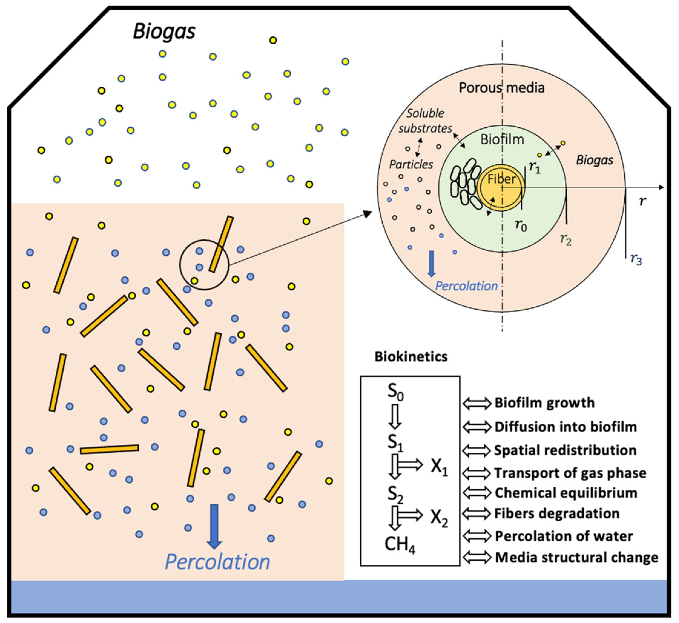
2.1. Different Phenomena Involved in SSAD

2.1.1. Biokinetics of Anaerobic Digestion

The first biochemical process of anaerobic digestion is hydrolysis. During this stage, the macromolecules contained in the substrate (mainly lipids, proteins and carbohydrates) are hydrolyzed into water-soluble monomers and oligomers with the help of enzymes secreted by hydrolytic microorganisms [17,18,19]. Depending on the substrate treated, the monomers obtained can vary (long chain fatty acids, amino acids, monosaccharides …). This first step is often considered the limiting step in AD for lignocellulosic substrates [20,21,22]. The second stage of the anaerobic digestion process is acidogenesis. The bacteria responsible for this step are the acidogenic bacteria. During this step, the products of hydrolysis are transformed into volatile fatty acids (VFA), alcohols (ethanol and propanol), carbon dioxide and partially into hydrogen. The acetogenesis step is the third step which consists of acetate formation from the products of the previous two steps. The final step in the anaerobic digestion process is methanogenesis. The microorganisms responsible for the methanogenesis stage are the archaea. They are microorganisms with metabolic characteristics and a membrane structure different from prokaryotic bacteria. Archaea are characterized by slow development and high sensitivity to pH. An ideal pH is between 6.5 and 8.5 for this step to avoid inhibition. All of these steps are schematically shown in Figure 2.
The modeling of the anaerobic digestion phenomenon represents here the methods allowing representing the temporal and spatial evolution of the compounds intervening in the anaerobic digestion process. There are different methods of approach to model this process and the objective of this part is to describe the models used. The kinetics of these reactions can take several forms depending on the experimental assumptions made and the complexity of the model. The reaction kinetics most used in the literature are detailed in Appendix A.

2.1.2. Phenomena of Transfer (Mass and Heat)

In addition to biological kinetics, various matters and heat transfer phenomena are also involved during anaerobic digestion. Mass transfer phenomena can be broadly divided into two categories: interactions between the different phases and hydrodynamic transfers. Although the latter always take place, they are only considered in modeling for solid anaerobic digestion, which, unlike liquid anaerobic digestion, is assumed to be highly heterogeneous.
  • Physico-chemical balances
Several physico-chemical balances exist within the anaerobic digestion process. There are balances between the phases throughout the degradation process, as well as chemical balances between the different species present. To understand the principle of physico-chemical equilibrium, it is necessary to review some notions of thermochemistry. The chemical transfers being independent, the equilibrium between two phases A and B is thus expressed by the equality of the chemical potential which comes back to the equality of the fugacity. Depending on the approach used (γ-ϕ or ϕ-ϕ), it is then possible to determine the equilibrium equations between phases according to the assumptions made. However, the use of thermochemistry in the field of anaerobic digestion is often limited to simplified phase exchanges and is only applied to liquid-gas equilibria, with the hydrolysis step producing monomers directly in their soluble form.
Equilibrium phenomena between liquid and gas phases are present within the anaerobic digestion process, especially during the CO2 and CH4 production steps. By performing a γ-ϕ approach on the chemical equilibrium between the liquid phase considered ideal solution and the gas phase and considering liquid mixture as an ideal mixture with low concentration of species in the liquid phase and pressure below ten bars, Henry’s law is obtained. Henry’s law is the most common liquid-gas equilibrium law used in SSAD modeling and is expressed in Equation (1) below:
P g a s , i = P S i V = K H S i L
where KH is Henry’s constant (mol·m−3·Pa−1), Pgas,i is the partial pressure of species i in the gas phase (Pa) and S i L the concentration of species i in the liquid phase (mol·m−3). Henry’s law thus represents the equilibrium between the liquid and gas phases in a stationary state. To describe the transfer phenomena between the liquid and gas phases, the double film theory of Whitman (1924) is the most commonly used. The assumptions made are to consider only the phenomenon of molecular diffusion in a stationary regime and when the contact time between the phases is greater than the time necessary to reach a stationary concentration profile. The expression of the transfer rate is then written in Equation (2):
v i , T = k L a ( S i L K H P g a s , i )
with v i , T as the velocity of the liquid-gas transfer (mol·m−3·s−1); k L as the transfer coefficient (m·s−1); a as the specific surface (m2·m−3); S i L as the concentration of species I in the liquid phase (mol·m−3); and Pgas,i as the partial pressure of compound i in the gas phase (Pa). Generally, the coefficient kL a is considered as a single constant because of the difficulties in determining the specific surface a and dissociating the two constants. Indeed, many parameters are to be considered such as the geometry of the reactor and the physical properties of the phases [20,23]. These phenomena play a very important role in anaerobic digestion because methane and carbon dioxide are first produced in the liquid phase before going into the gas phase [20]:
-
The liquid-gas material transfer directly influences the CO2 concentration in the liquid medium and thus the pH of the medium through the buffering capacity related to bicarbonates [24,25].
-
It also influences poorly soluble compounds (like CH4 and H2) can reach a concentration of 80 times that of thermodynamic equilibrium [26].
However, studies have shown that overpressure can be beneficial to the anaerobic digestion process, especially to overcome ammonia toxicity: the CO2 concentration in the liquid phase can decrease the pH by buffering effect [27].
Liquid-solid interactions are numerous in the AD process and are divided into two categories: sorption and precipitation. Hydrolysis is not considered since we consider the production of monomers from hydrolysis directly as solutes and not as solids. Adsorption is the process by which gas or liquid molecules attach themselves chemically or physically to solid surfaces. The causes of this attachment are surface reactions of a physical (capillary or hydrophobic repulsion), chemical (surface chemical reaction) or electrical (electrostatic or polarization interactions) nature [28,29,30]. The opposite phenomenon is desorption and can also occur in the AD process. There are links between the decrease in the concentration of certain aromatic components such as humic acid with the organic content of the solid phase, but the multitude of substances involved makes characterization of these phenomena difficult [29,30]. In anaerobic digestion processes, the lignocellulosic substrate content gives an indication of the adsorption of hydrophobic organic molecules due to the polar character of lignin [31]. This means that lignin contributes to the isolation of potentially toxic compounds for the anaerobic digestion process. Few studies have been conducted on this subject [32] in contrast to biosorption, which is the phenomenon representing the formation of bonds between dead biomass and heavy metals present in the digestion medium [31]. These mechanisms are related to the extracellular polymers produced by the bacteria and studies have been conducted on the biosorption of various heavy metals [33,34]. These sorption phenomena are therefore of interest for anaerobic digestion because, in the right proportions, they avoid inhibition by heavy metal concentrations [35]. Precipitation is a phenomenon arising from the complexation of ions in neutral inorganic form [32]: calcium carbonates, calcium phosphate, sulfato-metallic precipitates and phospho-magnesium complexes are the most commonly encountered in the methanization process [36]. Precipitation leads to various problems: it reduces the useful volume of the digesters, reduces microbial activity by cementing the biomass and impacts the production rate of biogas and digestate [37,38]. Precipitate formation is related to pH, soluble mineral concentration and process temperature, so it is necessary to control these parameters to avoid negative impacts of the precipitation phenomenon [20]. Physico-chemical studies could allow a better control of these phenomena.
  • Mass balances and hydrodynamics behaviors
The creation of a mathematical model requires the construction of equations representative of the studied phenomenon. For partial differential equation models, some considerations, mass balances for each solute have to respect a global mass balance (Equation (3)):
I n p u t + P r o d u c t i o n = O u t p u t + A c c u m u l a t i o n
Being adapted to each chemical and biological species, the mass balances make it possible to build mathematical models representative of anaerobic digestion in the solid process. In these models, two main types of hydrodynamics phenomena could be considered: diffusion and convection phenomena. These phenomena are represented by local variations of a solute C and expressed by the following Equations (4) and (5):
C t = q C z
C t = D 2 C z 2
where C represents the solute concentration (kg·m−3), q the Darcian velocity (m·s−1), and D the diffusion coefficient (m2·s−1). These equations are present in heterogeneous modeling representing spatial variation of each solute.

2.2. Theoretical Models

Theoretically, an AD reactor involves enormous physical, chemical and biological phenomena. The complexity of modeling increases when it comes to the SSAD system. The heterogeneity in solid media and the interactions between different phases are to be taken into account. This leads to the use of partial differential equations (PDE) in the model in order to characterize the dependence of various variables not only on the time (t) but also on the space (coordinates). Since the modeling of AD was developed at first according to LSAD system where heterogeneity in reactors is less concerned, it is usual that the spatial variation of the variables is neglected supposing a (quasi-)homogeneous system or a perfect mixed one, which simplifies PDE to ordinary differential equations (ODE). This reduces the complexity of the model and the time for the calculation.
When modeling techniques are adapted from LSAD to SSAD, the hypothesis is at first established that the system is mixed so that the complexity of modeling could be reduced when a multiple of phenomena are considered. Afterwards, the spatial effect is specified and introduced into the system to represent better the reality of a SSAD system with heterogeneity of materials in the reactors. There also exist some special models in which a non-conventional theory is given to describe the reactions or the physics in the SSAD reactors.
This chapter is dedicated to a literature review about the modeling of SSAD in perfect mixed systems (with time-depending ODE), heterogeneous systems (with time- and spatial-depending PDE). The use of non-conventional theories for modeling is also introduced in this part.

2.2.1. Perfect Mixed Systems

Table 1 gives a summary of the literature review of the simulation studies on SSAD supposing a perfect mixed system. Generally, these studies can be categorized into the conventional biochemical modeling using ADM-1 type models or the non-conventional models proposing new theories explaining the phenomena. Various effects such as TS content, gas/liquid equilibrium and mass transfer could be considered in the modeling.
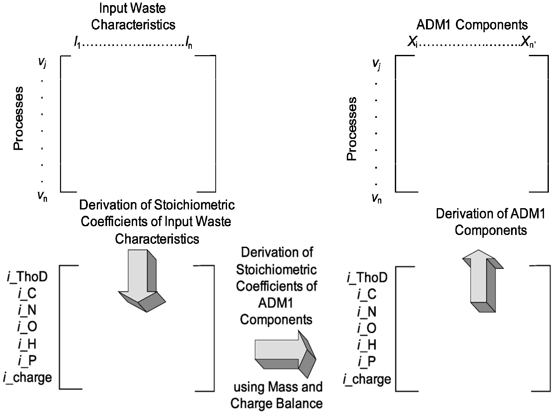
  • Biochemical dynamic modeling (ADM1 and its derivatives)
The ADM1 model is the most-known AD biochemical model [20]. It allows a good simulation of the LSAD reactors but requires the identification of a large number of kinetic and physico-chemical parameters. ADM1 has many variants and simplifications for LSAD system [39,40,41]. AM2 proposed by Arzate et al. (2016) [42] is one of the simplified ADM1 with only two microbial populations involved and listed as follows: acidogenesis and methanogenesis. Hydrolysis step could be added prior to AM2 model to complete a full degradation chain of substrate. Sari (2022) looked into the simplified one stage or two-stage models capturing the major behaviors of full ADM1 model [43]. ADM1 and its extensions have also been adapted to the SSAD simulation since long.
Bollon et al. (2011) [44] simulated the SSAD processes of organic fraction of municipal solid waste (OFMSW) by developing a ADM1-type kinetic model considering acetate degradation and moisture content of the medium. This model modified ADM1 by putting hydrolysis and acidogenesis stages in one first-order kinetic equation. The innovation of the study was found in the 3-liquid-gas dynamic equilibrium of CH4, CO2 and H2. The batch methane production of acetate was simulated (Figure 4 of [44]). Results showed that the methane yield was limited by the mass diffusion of soluble matter. They also concluded that the kinetic parameters of ADM1 in conventional LSAD were not adequate to describe SSAD reactions.
Abbassi-Guendouz et al. (2012) [45] studied the effect of Total Solids (or dry matter) on the SSAD of cardboard. The modeling using ADM1 model was also carried out. They mentioned that the default value of first-order hydrolysis rate (10 d−1) was not sufficient to simulate SSAD and a very low hydrolysis kinetics (0.1 d−1) according to Qu et al. (2009) [46] was considered.
The model developed by Liotta et al. (2015) [47] was based on the ADM1 modified by Esposito et al. (2008) [48]. There were 28 sets of mass balance equations. One particular parameter characterizing disintegration of complex OM (Ksbk) as well as two kinetic parameters for acetate and propionate (Kac and Kpro) were reckoned to be a linear function of the Total solids content (TS) of the media. This helps the adjustment of the kinetic parameters according to the feedstock of digesters (food waste, straw …).
A modified AM2 model suggested by Attar and Haugen (2019) [49] took into account the difference of inflow and outflow rates, the effect of temperature on the specific growth rate and a mass and charge balance for inorganic carbon content estimation. Faced up with the real-scale experimental data, the modified AM2 was proved sufficient to accurately predict the biogas production behaviors of sewage sludge. A sensitive analysis was also accordingly performed to examine the dominant parameters impacting the variables.
Table 1. Summary of simulation studies on SSAD processes supposing a perfect mixed system.
AuthorsSubstratesReactor ModeHydrolysis KineticsMajor BiokineticsSpecial ConsiderationMass Transfer
Kalyuzhnyi et al. (2000) [50]/N.A.First-order kineticEquilibrium-based kineticspH, gas/liquid equilibriumDiffusion
Martin (2000) [51]/N.A.Expansion of reaction shellsRate proportional to volume of shells//
Martin et al. (2003) [52]/N.A.Taking place in acetogenic zoneReaction front mechanism7 mobile zonesDiffusion
Bollon et al. (2011) [44]OFMSW
gAcetate
BatchFirst-order kineticsModified ADM1gas/liquid equilibrium of CH4, CO2 and H2/
Namuli et al. (2011) [53]Dairy farm wasteN.A.Stoichiometric modelADM1Density, CHNSO, VS, ash, N, P and K contents/
Fdez-Güelfo et al. (2011, 2012) [54,55]OFMSWSemi-continuous/Modified Monod-type equationNon-biodegradable substrate concentration/
Abbassi-Guendouz et al. (2012) [45]CardboardBatchFirst-order kineticsModified ADM1Kinetic parameters adjusted by TS/
Xu et al. (2014) [56]Corn stoverBatchFirst-order kinetic with inhibitionModified GompertzAdjustment of Gompertz parameterDiffusion
Liotta et al. (2015) [47]Food waste
gRice straw
BatchFirst-order kineticModified ADM1Kinetic parameters adjusted by TS/
Poggio et al. (2016) [57]Green waste
gFood waste
Batch and semi-continuous First-order kineticADM1CHNSO contents, Nitrogen, COD/
Attar and Haugen (2019) [49]Sewage sludge//Modified AM2Liquid level change, temperature/
Lafratta et al. (2021) [58]Sewage sludge
gDog food
ContinuousFirst-order kineticFirst-order kineticsFirst-order kinetics for all biochemical reactions/
  • Stoichiometric model combined with ADM1
Another tool considering the characterization of input waste was developed by Namuli et al. (2011) [53]. In this study, the density, the elementary fractions (CHNSO), the ash, phosphor, potassium and VS contents were fed into an ADM1-type model allowing calculating the final biogas yield through mass and charge balance (Figure 3).
Similarly, Poggio et al. (2016) [57] combined ADM1 with a biochemical fractionation. The carbohydrates, proteins and lipids fractions were obtained by realizing nitrogen, COD and mass balances. The first two balances were realized based on the elemental characterization (CHNSO contents) of the raw substrates. The batch test data of green waste and food waste were used for the model calibration. The model was then validated using a semi-continuous dataset (cf. Figure 8 of [57]). A good prediction of various variables like biogas production, VFA, total nitrogen and alkalinity were achieved.
  • Two-particles model
Kalyuzhnyi et al. (2000) [50] developed a structured mathematical model of SSAD process by dividing the solid media into two particles as “seed” particles and “waste” particles. The “seed” particles had low biodegradability and relatively high methanogenic activity. On the contrary, the “waste” particles had relatively high biodegradability but is low in methanogenic activity. The organic solute could be transferred from one particle to another by diffusion. Diffusion was carried out by Fick’s Law-like equation. Both kinds of particles were supposed to be in a perfect mixed system. Stoichiometric reactions, microbial development, liquid-gas equilibrium and pH issues were considered in the model.
  • Reaction front model
Martin (2000) [51] simulated the SSAD reactions taking place on an imagined interface between the raw and digested waste. This work considered the expansion of hydrolysis or acidogenic shells whose growth rate was proportional to the production rate of biogas. This innovative model fitted the experimental data well as compared with the first-order decay kinetics. This non-conventional approach was then further developed by the same author and named “the reaction front hypothesis” [52]. The new theory proposed a leading zone where acetate was formed as well as a methanogenic buffered zone where acetate was diffused. These seeding zones could grow gradually until the process stabilization. This very novel concept of modeling opened the perspectives about using non-mechanistic theory for modeling of a complex multi-physical system such as SSAD.
  • Simplified Monod model
The studies of Fdez.-Güelfo et al. (2011, 2012) [54,55] worked on the process modeling of dry thermophilic AD of either simulated or real OFMSW by using a simplified Monod-like equation (Equation (6)):
r s = μ max ( h S ) · ( S S NB ) ( S S NB )
where −rs is the substrate consumption rate (g·L–1·s–1), μ max is the specific growth rate of microorganisms (d–1), S is the concentration of substrate (g·L–1), h is the maximum concentration of substrate that could be achieved (g·L–1). The kinetic parameters could be obtained by the non-linear regression of the methane yield curves. They succeeded, by using their model, in obtaining the μ max and the minimal sludge retention time for a stable operation of SSAD.
  • Mass diffusion model combined with empirical equation
A mass diffusion model was developed by Xu et al. (2014) [56]. In this model, the hydrolysis step was assimilated to the first-order kinetic with inhibition terms. The mass diffusion model used Fick’s Law to simulate the diffusion flow rate of sugar into microflora. A mass balance between the substrate and inoculum layers was also taking into consideration. The degradation of sugar inside the microbial cells followed a simplified Monod equation. Instead of going into complex biochemical simulation, they used the modified Gompertz equation to achieve the final biogas production (cf. Figure 2 of [56]). However, its maximum methane production rate was achieved by the following equation (Equation (7)) considering the hydrolysis, diffusion and inhibition phenomena:
( R CH 4 ) max = k h X F 0 Y Δ C H 4 / Δ S k i k s Y Δ M / S μ max X M 0 + k i L V D e A + 1
where (RCH4)max is the maximum methane production rate (NmL CH4∙g VS−1∙d−1); kh, ki and ks are the hydrolysis, inhibition and substrate half saturation coefficients (d–1); X M 0 and X F 0 are the initial substrate and inoculum concentrations (g·L–1); Y Δ C H 4 / Δ S and Y Δ M / S are the microbial growth yield and methane yield coefficients (−), De is the diffusivity of sugar; and L, A and V the thickness, surface and volume of substrate layer. The obtained (RCH4)max is injected into a modified Gompertz equation for methane production curve (Equation (8)):
P ( t ) = P 0 / { 1 + exp [ ( R CH 4 ) max · e · ( λ t ) / P 0 + 1 ] }
where P(t) is the cumulative methane yield at day t (NL CH4∙kg VS−1), P0 is the simulated methane yield of the substrate (NL CH4∙kg VS−1), e is Euler’s number (e = 2.71828...), λ is the lag time (d) and t is the digestion time (d).
  • First-order dynamic model
A first-order dynamic model was developed by Lafratta et al. (2021) [58] supposing all of the biochemical reactions follow the first-order kinetic. They suggested that first-order kinetics had fewer parameters to identify and thus could make the simulation less heavy by achieving the similar accuracy. The modeled values fit well the experimental data (cf. Figure 8 of [58]).
According to the literature analysis above and the information provided by Table 1, it is interesting to note that most of the modeling is based on the ADM1-type model for biochemical simulation. The phenomenon of diffusion or convection is not systematically included since the hypothesis of a perfectly mixed reactor limits the role of mass transfer in describing the reactions inside a solid-state digester. The consideration of a heterogeneous system with a multidimensional approach would be more appropriate to introduce the mass transfer into the modeling.

2.2.2. Heterogeneous Systems

It is difficult to transpose the biokinetics used for liquid anaerobic digestion to solid anaerobic digestion. Indeed, the low-free water content in digesters [59] and the lack of knowledge on the mobility of microbial species and their mode of action in this environment limits the development of models for this phenomenon [32]. Hydrodynamic-related phenomena influence reaction kinetics by impacting material transfers and percolation within the solid mass [60].
  • Distributed model
According to the different models presented, a one-dimensional distributed model has been developed considering diffusion and convection transfers within the liquid phase [61]. This model assumes homogeneity according to the cross-section of the reactor used and a variation considered only along the reactor. This model (Equations (9)–(12)) uses a system of partial differential equations including spatial and temporal variations to consider the transport phenomena and the biological kinetics of the process:
X t = k H X f ( S )
S t = D S 2 S z 2 q S z + k H X f ( S ) ρ max S B K S + S g ( S )  
B t = D S 2 B z 2 q α B z + Y B S ρ max S B K S + S g ( S ) k D B  
G t = γ ( 1 Y B S ) ρ max S B K S + S g ( S )  
with X, S, B and G (kg·m−3) as the solid substrate, soluble substrate, microorganisms and gaseous products, respectively. The term γ represents the fraction of methane in the biogas and α represents the fraction of biomass carried away by liquid convection. DS represents the diffusion coefficient (m²·s−1) and q the Darcian velocity (m·s−1). The terms ρmax and KS are the constants related to the Monod kinetics. The terms g(S) and f(S) are the inhibition functions related to acetogenesis and hydrolysis, respectively. Obviously, other studies have been carried out with the distributed model using different biological kinetics such as the Contois model for hydrolysis or by dividing the solid substrate into several species with different hydrolysis kinetics [62,63]. The consideration of transport phenomena by a distributed model is thus a complete approach allowing an adaptability of the biological kinetics and a modification of the model according to the working assumptions.
  • Spatio-temporal model
The space-time model was developed to take into consideration the heterogeneous distribution of biological kinetics and spatial distribution of substrates [64] by extending the use of the distributed model to 3D, this model includes the phenomena of material transport, and allows to show how the spatial distribution affects the degradation of the material, in particular for solid-state anaerobic digestion. The equations of this model (Equations (13)–(16)) are therefore very close to the distributed model:
X t = D X Δ X a 1 q X b 1 X f ( S )
S t = D S Δ S q S + k 2 X f ( S ) b 3 B g ( S )  
B t = D S Δ B a 2 q B + b 4 g ( S ) B b 5 B  
G t = D G Δ G q G + b 6 g ( S ) B  
with a1 and a2 are the fractions of substrate and biomass carried away by liquid convection, and the b1b6 are the reaction terms used here as constants to be determined to simplify the model [65]. There are other models developed from the presented models, such as the diffusion limit model [56] considering the effect of the proportion of dry matter on AD; but, as ADM1, the main theoretical models are those cited above.
  • Mobile-Immobile model
The work of Coutu et al. (2022) [66] simulated the SSAD of cattle manure in a leach-bed reactors. They proposed a novel model coupling Mobile-Immobile water interactions (MIM) and AM2. Another novelty was related to the consideration of the microporosity and macroporosity evolutions of solid bulk, found by Hernandez et al. (2021) [59], in the coupled model. The theoretical model was created based on a one-dimensional diffusion-like theory in which the immobile fraction of OM is hydrolyzed and diffused into mobile zone for biodegradation (Equations (17) and (18)). The realization of the model in the paper was conducted supposing perfect mixed system and therefore, reduced to a zero-dimensional model (independent of spatial effect). The fitting of the simulated data to the experimental values is rather satisfactory (Figure 4).
θ m ( t ) t [ C m i ( z , t ) ] + C m i ( z , t ) t [ θ m ( t ) ] + α [ C m i ( z , t ) C i m i ( z , t ) ] = θ m ( t ) D ( t ) 2 [ C m i ( z , t ) ] z 2 q [ C m i ( z , t ) ] t + θ m ( t ) j = 1 M σ j r m j ( z , t )
θ i m ( t ) t [ C i m i ( z , t ) ] + C i m i ( z , t ) t [ θ i m ( t ) ] = α [ C m i ( z , t ) C i m i ( z , t ) ] + θ i m ( t ) j = 1 M σ j r i m j ( z , t )
where θm and θim are the mobile and immobile water fraction of the bulk (m3·m–3), Cm and Cim are the concentrations of soluble matter in mobile and immobile zones (kg·m–3), α is the coefficient of mass transfer between mobile and immobile zones, i is each soluble matter species, σj is the stoichiometric coefficient of each soluble matter considered in the reaction j, rmj and rimj are the reaction rates for reaction j in mobile and immobile zones (kgCOD·m–3·d–1).
  • Gradostat models
Another way of modeling is to approximate spatialization using a set of simple interconnected models. This is the case of gradostat models, considering a set of two or more interconnected steady-state reactors called chemostats. Each chemostat is a two-way flow between input and output [67]. The gradostat models appeared during 1950s as a representation of the microbial growth in steady-state reactors [68,69]. Modeling of each reactor considered substrate and biomass concentration, respectively, respecting the following equations:
d s d s = 1 Y μ ( s ) x Q V ( s i n s )
d x d s = μ ( s ) x Q V x
with x and s the substrate and biomass concentrations, Q the input flow, V the effective volume, Y the yield conversion of substrate into biomass and µ the specific growth rate of micro-organisms. Many studies were led using this tool [70] to describe bioreactors with an easy spatial discretization allowing avoiding partial differential equations resolution.
  • Plug flow simulation
Most of the simulation is realized in batch mode. The work of Panaro et al. (2022) [71] studied the modeling of SSAD process in plug flow reactors. The convective and diffusive phenomena were included in the one-dimensional flow. An AM2-type biochemical model was applied to simulate the biodegradation of organic matter and the production of biogas. The simulated data were confronted with the experimental results and showed good accuracy.

3. Statistical Approaches

3.1. Empirical Non-Linear Regression Models

Most of the models used in solid-state anaerobic digestion propose theoretical approaches. The advantage of these methods is to increase the understanding of the phenomenon and to allow a simple prediction of the degradation of the substrates. The disadvantages are that they present a certain complexity, which can limit the identification of the kinetic parameters of the model and move away from the experimental reality [72]. In order to predict methane production in a simpler way, some models use an empirical approach described in this section.

3.1.1. Logistical Model

The purpose of the logistic model is to propose a simplified model to reduce the number of parameters and make them more easily identifiable. This model introduces several assumptions which are the following:
-
Only biomass concentration induces methane production.
-
Biomass growth is limited by factors such as hydrolysis rate and substrate availability.
-
Inhibition and death of microorganisms are not taken into account.
-
The proportion of liquid adsorbed on the solid substrate and present in the capillaries is not accessible to microorganisms and solutes.
The model obtained is the following Equation (21):
d B d t = μ max B ( 1 X 0 max X X 0 )
with B the biomass concentration and X the solid substrate concentration (kgCOD·m−3), μmax being the maximum growth rate and thus the only model parameter to be determined (s−1). In this model, water is assumed to be adsorbed onto the solid matrix and capillaries are unavailable areas for solute and microorganism transport. Two parameters are assumed to correlate with the microorganism concentration: the maximum growth rate μmax and the initial amount of available organic matter X0. The water content ω is considered empirically in Equations (22) and (23):
μ max = τ μ max R
τ = ω ω 0 ω R ω min
where τ is a function in which ω0 represents the initial water content, ωR the maximum water content and ωmin the minimum water content to ensure bioconversion initialization. These equations suggest that if the water content reaches the maximum allowable water content, all of the substrate X0 is available for AD. Below this, methane production will not reach its optimum [72].

3.1.2. General Kinetic Model

A model (Equation (24)) was designed by Fernández et al. (2010) [73] and developed by Fdez-Güelfo et al. (2012) [55]. This model, called the general kinetics model, consists of a simplification of the reaction rate law:
B + X Δ ( Δ > 1 )
where X (kg·m−3) is the organic carbon concentration in the solid substrate, B (kg·m−3) is the microorganism concentration, and Δ is a stoichiometric constant. The equations specific to the evolution of the state variables are therefore (Equations (25) and (26)):
d B d t = ( Δ 1 ) k X B
d X d t = k X B
with k the reaction rate constant associated with the process (kg·m−3). Considering the initial substrate concentration X0, the non-degradable substrate concentration XNB, the maximum growth rate μmax and h the maximum concentration of microorganisms, the last equation can also be written in Equation (27):
d X d t = μ max ( h X ) ( X X N B ) X 0 X N B  
Concentrations here are expressed in kgCOD·m−3. The combination of the substrate degradation rate and the methane production rate gives the Equation (28):
G = Y G X ( e θ t 1 1 h X 0 + e θ t X 0 X N B )   with   θ = h X N B X 0 X N B
here G represents the total amount of methane produced and YG/X the yield of methane produced per unit of substrate consumed (m3CH4·kgCOD−1). This model has been used to study the impact of dry matter content on the solid-state AD process. Fernández et al. (2010) [73] found a maximum degradation rate almost twice as high at 20% dry matter than at 30%. These findings are similar to those in the literature on the impact of dry matter content on methane production [45,47]. The kinetics of this model were then modified by Fdez-Güelfo et al. (2012) [55] to adapt it to thermophilic conditions with validation on two types of substrates and four different types of feedings. More generally, empirical models are based on modifications of the Gompertz equation and the logistic equation, which are the two frequently used empirical models [74,75,76]. These two models provide some representative parameters such as the lag time, also called lag phase, or the maximum degradation rate. The modified Gompertz model seems to have a better match with experimental results than the other empirical models, but there are few comparisons on solid-state AD modeling [74,76,77].

3.1.3. Non-Linear Regression Models

In multiple linear regression models, each studied parameter i is represented in the model by a variable xi and a coefficient ai. The observed response y is usually methane production. The value of the coefficient is used to give a tendency for the observed variable favor increasing or decreasing the response. The regression generally goes up to second-order terms, with higher-order terms no longer making physical sense. The general expression for this model is in Equation (29) as follows:
y = a 0 + i = 1 k a i x i + i = 1 k a i i x i 2 + i , j = 1 i j k a i i x i x j
The coefficients ai represent the coefficients of each variable xi, also called factor. The a0 represents the response value under the average conditions of the study domain of the different variables. The coefficient aii represents the quadratic coefficient of the quadratic factor xi2 and aij represents the impact of the interaction of parameters i and j. These models are used in the design of experiments methodologies for the representation of the response surface. These models have been used in the context of anaerobic digestion to evaluate the impact of many parameters on methane production. The studies carried out on the anaerobic digestion process and using the design of experiments methodology have multiplied in recent years, allowing a better understanding of the optimal operating conditions of the anaerobic digestion process. The studied parameters are in particular the following:
-
Optimal pretreatment conditions on the efficiency of anaerobic digestion [78,79].
-
The optimal conditions for liquid phase recirculation under solid-state anaerobic digestion conditions [80].
-
The determination of the optimal values of carbon to nitrogen ratio [81].
-
The determination of the optimal pH [82].
-
The determination of optimal biomass inoculation conditions [83,84,85,86].
There are also more complex studies such as optimizing digester geometry to maximize methane production [87]. Factors can also be linked together by constraints such as the fundamental mixing constraint. This allows for optimization of process methane production by acting on the composition of a mixture. Such work has been conducted on AD [88,89] considering up to three different substrates. Another possibility is to optimize both the substrate composition and the values of the operating parameters by mixing different regressions [90]. The limitation of such a design of experiments is the increasing number of experiments required for each additional substrate. The different parameters studied are shown in Table 2. Other responses can be studied, such as VFA production, or pH. Some studies are multi-response and subsequently optimize an objective function that skillfully combines these different responses [91]. Multilinear regression has been shown to be a very useful tool for predicting methane production from different substrates [92,93]. It is also an inexpensive tool to implement in terms of time and technique. It is then the ideal strategy to “rough out” the parameters of interest in order to determine the significant variables to study.

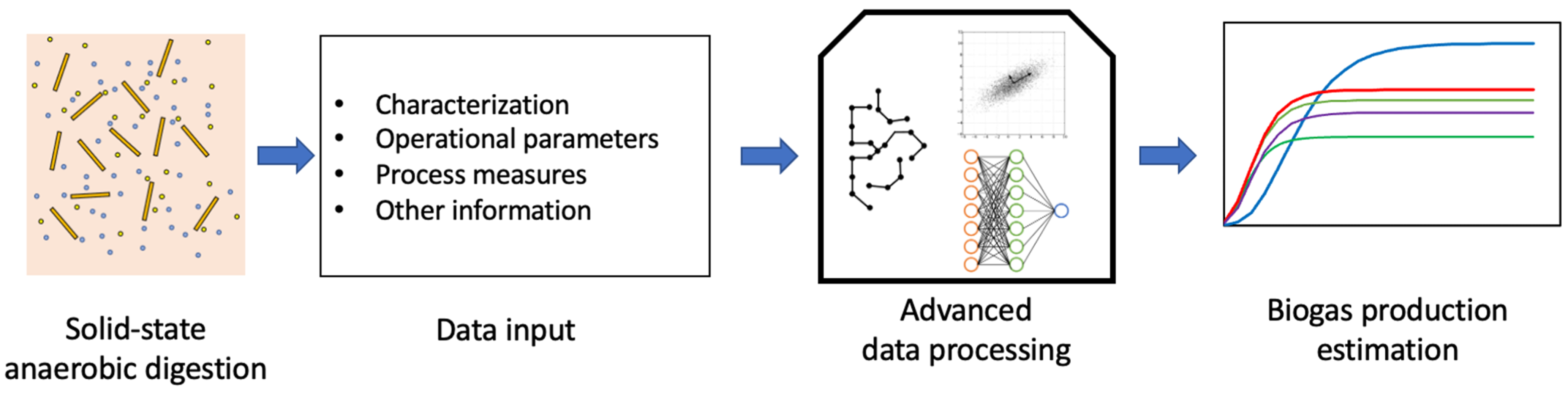
3.2. Advanced Statistical Models

In addition to non-linear regression models, the chemical engineering industry is seeing its increasing interest in the use of machine learning for process modeling. It is somehow a black-box approach, or considered as phenomenological modeling (Figure 5). These models do not give directly mechanistic explanation of the simulated phenomena, which, at least, is not the prioritized purpose of these models.
The machine leaning approach (including artificial neural network, ANN) has been largely studied to predict the performance of wastewater treatment plant [94], the process of upflow anaerobic sludge blanket process (UASB) [95], the LSAD of sewage sludge [96], industrial sludge [97] and agricultural byproducts [98].
A few studies using machine learning are available for SSAD simulation.
Xu et al. (2014) [99] collected 50 datasets from 10 publications as data input, including the physico-chemical features of the substrates and the inoculum (pH, TS, VS, TN, sugar, cellulose and lignin contents …) as well as the operational parameters of the SSAD processes (temperature, C/N ratio, particle size, substrate/inoculum ratio…). Three ANN models were used. The first model used all of the collected parameters as input. The second one used the crucial parameters that are found significant by the multilinear regression. The last one used the parameters that could be easily obtained or realized like VS, TS, C/N ratio. All three models were calibrated by one part of datasets and validated by another part. The authors stated that more datasets were required for a better training of the model.
Seo et al. (2021) [100] tried to predict the biogas yield rate from continuous SSAD of food waste with the aid of the process-wise modeling or the neural network approach. The sludge retention time (SRT), soluble COD, total VFA, total ammonia-nitrogen (TAN) and free ammonia are used as model input. Compared to process-based model, the neural network method was more efficient in the prediction of biogas yield from food waste in SSAD reactor (cf. Figure 6 of [100]).
A very recent paper of Pei et al. (2022) [101] tested extreme machine leaning (EML), ANN and random forest (RF) for SSAD modeling. The RF method found three critical parameters (butyric acid, acetic acid and pH) impacting the biogas yield. Best prediction accuracy was obtained by the algorithm of EML (Figure 3 of the [101]).
The algorithm of the machine learning modeling is still undergoing fast development. It is evidenced that theses could be a very useful tool for accurate estimation and thus a finer control of the process behaviors of biogas production, without entering the very details explaining what is happening behind. A large quantity of data input, which cannot be easily acquired, is indispensable for a better training of the model. A shared database of anaerobic digestion data on various scales would be greatly helpful for a larger development of the field [9].

4. Discussion and Perspectives

4.1. Limitations of Current Modeling Methodology

4.1.1. Modeling Approaches

As discussed above, either theoretical or statistical approaches are efficient in SSAD modeling. Without specifying the objectives of the modeling, it would be difficult to privilege one over another.
  • Theoretical models
The modeling can serve for a better understanding of the physico-chemical and biological phenomena taking place in the reactors. In this case, the theoretical approaches with a better vision on the intermediary processes or products would be preferred. This approach allows the interpretation of results supported by the scientific explanations. However, one has to note that the good outcome of theoretical models only shows the fit of theory to the experimental observations. It would not be reflecting the reality in the reactors. For the same experimental results, a multiple of theories could apply. The identifiability of parameters (to be discussed later) may also bring the difficulty in using theoretical models by nonacademic specialists. Furthermore, the theoretical models usually require some strict hypotheses. This means that the use of this model from one type of reactor to another, from one kind of substrate to another and from one mode of operation to another would vary to a great extent. It may limit the use of the modeling of this kind for industrial applications facing the complexity and variability of substrates in real biogas plants.
As specifically for SSAD, the development of theoretical models is therefore of great challenge for researchers to be able to understand a complex system with a variety of the physico-chemical phenomena involved. The combination of the mass transfer and biokinetic equations with a hydrodynamic model is difficult to put into service since for a small SSAD reactors there could be millions of cells to be numerically simulated, taking a considerable time for the simulation.
  • Empirical and advanced statistical models
The statistical methods provide another way to simulating SSAD processes. Whichever grey box or black box modeling, the statistical approach does not pay as much attention as the theoretical approach does to the intermediary products or individual phenomena (i.e., CFD, mass and transfer, biokinetics). The understanding of the processes is not the first objective of the modeling. The SSAD is such a complex system that, as discussed for theoretical models, the combination of different physico-chemical phenomena in one model would be difficult to realize in an efficient way and within a reasonable simulation time. This makes the empirical and advanced statistical models stand out since these tools need less information about specific physics and avoid to enter the details of the reactions.
The nonlinear fitting of empirical equations to the experimental data often shows good simulation of biogas production. It is an easy tool for the use and comprehension for non-specialists. However, the extrapolation of the models would not be simple and accurate. The overfitting problem has to be noted and taken care of [102]. Besides, the empirical models with limited equations are always doubted to be sufficient to describe a reactor as complicated as SSAD. Information may be lost when using simple empirical models.
The advanced statistical methods, such as random forest and neural network, are very robust and promising tools for SSAD simulation. The quality of modeling highly depends on the volume of training datasets. For a biogas plant with a large amount of data (measures in hours over several years), these tools can be efficient to predict possible inhibition and digestion failure so that the handling persons can react in time.

4.1.2. Mathematical Model Implementation

The first step of model development is the mathematical model implementation. Every assumption and consideration must be done in this part to determine limits and possibilities according to the goal of the study. Concerning solid-state anaerobic digestion, different physical and biological phenomena could be considered as biokinetics and hydrodynamics. Units must also be determined for the study. In fact, concentrations could be expressed in mass, moles or COD, as space and time measurement must be adapted considering the phenomenon scale. Different factors could be considered as the substrate properties in terms of possible inhibitions, the liquid phase recirculation frequency or rheology to adapt hypothesis of the study. At this point, a verification step is necessary to ensure a correct mass balance between solutes, substrates and biomass. This verification step could be done by a derivation of the global mass balance equal to zero, ensuring a constant mass balance [66].
Moreover, the complexity of the dynamic systems of the bioprocesses imposes a rigor on the determination of the kinetic parameters related to the developed model. Considering heterogeneous systems, the identifiability of parameters is an important issue that must be treated for each developed model. Identifiability question is divided into a problem of structural identifiability and practical identifiability [103]. Structural identifiability is the study of the mathematical identifiability of each parameter in the case of ideal measurements. Different methods could be used to mathematically determined each parameter as transformation of the non-linear model into a linear model [104], development into series [105,106] or study of the observability of the nonlinear system [107].
Most of the theoretical approaches rely on the use of ADM1-type models for the biokinetic simulation. However, ADM1 is a large-scale non-linear model. The full version of ADM1 model deals with 19 reactions with a total 32 dynamic state variables. There are two types of parameters in ADM1 model: the biochemical parameters and the input or initial condition parameters [108]. The biochemical parameters derive from the model structure and can be obtained by calibration using appropriate experimental data. The calibration involves an optimization process through the minimization of an objective function, usually called “the fitting goodness” [109]. The study of Nimmegeers et al. (2017) [110] discussed about two identifiability, namely the structural identifiability and practical identifiability. The structural identifiability describes the availability of a unique estimation of parameters from a mathematical point of view on the structural of the concerned model. The practical identifiability refers to the estimation of parameters considering all identification conditions such as the quality of the input experimental data. The authors presented a reaction network of ADM1 and stated the complexity of the model with the parameters in large number makes the practical identifiability difficult to achieve. This nature could result in the multiple optimal outputs (i.e., non-unique set of parameter estimates) during the calibration. The parameters found could be intercorrelated. They suggested that, in order to make the parameter estimations locally and structurally identifiable, one should modify the ADM1 model by using the parameters combination instead of individual parameters. A good and adapted experimental design is also required to increase the practical identifiability of the parameters.
Unfortunately, in many practical cases it is not possible to identify the different kinetic parameters because of the poor quality and limited number of experimental data [111]. In these cases, it is then necessary to perform a sensitivity study on these parameters in order to determine the effect of a small variation of these parameters on the adequacy between model and experimental data [66]. This is why it is very important to implement a mathematical model before conducting any experiment to ensure a great identifiability of each calibrated parameter.
The SSAD modeling differs greatly from the conventional LSAD. The simple use of literature values of parameters obtained from LSAD modeling is not representative for SSAD due to its multiphase and multiphysical natures. This added one more difficulty in the simplification of the model calibration (to be discussed later).
A comprehensive database of anaerobic digestion of all kinds shared within the scientific and industrial communities would be of great help in enriching the available and adapted data for model training.

4.1.3. Calibration, Validation and Outcomes of Models

Two different datasets must be used to calibration and validation step to ensure a representative and reproducible model of the observed phenomenon. Different strategies could be used to minimize the number of experiments: dividing a dataset into two set of data, or create a dataset from existing database with numerical methods as bootstrapping [90]. Once mathematical model was implemented, kinetics identifiability was studied and datasets were identified, experiments could be realized.
Calibration step of kinetics parameters aims to obtain the best fitting with experimental data. Different methods could be used to calibrate kinetics on a dataset as mathematical regression for linear equations or a minimization of an objective function for complex linear equations system [90]. In this last case, initialization of kinetics could be very influential on calibration results. This is why initialization step is a critical point to ensure a great kinetics calibration.
Validation step is used to validate the calibration results previously obtained. A tolerance on the uncertainties obtained between calibration results and validation results must be determined before practicing validation step to ensure a robust correlation. This tolerance depends on the studied phenomenon. Future research should take into account this aspect when one designs the experimental variables and parameters to be determined.
The quality of modeling outcomes depends on the type of models used and the suitability of the training data for the model calibration. It is highly possible that the modeling results are only valid for the conditions with which the models are fitted and calibrated. The outcomes from model extrapolation would be highly uncertain and unreliable, making the modeling not ready for industrial ends. A big data volume and a good data representability are of great significance for the quality of the model, especially for the advanced statistical models like neural network.

4.1.4. Difficulty in Multiscale Modeling

The multiscale modeling concerns more the theoretical models. On one hand, the mass transfer and biokinetics occur on microscopic scale. The thickness of biofilm is less than 200 μm [12]. The relevant modeling is accordingly designed on this level (in micrometers or millimeters). However, when simulating the biogas production of real-scale reactors, usually in liters or in cubic meters, the microscopic model seems to be too small to take into consideration the heterogeneity of the digesting bulk [112,113]. Other models, like CFD [114,115,116,117,118], are usually based on real-scale modeling, suggesting the elements not going to the millimetric scale. The number of elements would be too many and the simulation is practically not possible if the mesh of real scale simulation consists of microscopic scale mesh. On the other hand, the temporal scale is varying depending on models. The CFD could be on second-wise (if possible) but the biokinetics including mass transfer, substrates degradation and the microbial growth are in days. These spatial and temporal scale differences call for further studies on multiscale transition and coupling of different models.

4.2. Lack in Knowledge of SSAD Reactors

4.2.1. Evolution of Media

Different from LSAD, SSAD media (bulk) are closer to the properties of solid and can be characterized by the parameters like size, density, apparent and bulk density, permeability and porosity. Theses parameters change as anaerobic digestion pursues [59,119]. This characteristic makes the development of mathematical models even more difficult since the parameters normally considered constant can no longer be put outside of the derivative terms, but turn to be a function of time (or other variables). In the reality of SSAD, the modification of media porosity and structural strength may give rise to the collapse of solid bulk, which is interpreted as the reduction in bulk height and volume. The consideration of these factors changes the simulation methods and amounts to the complexity to solve the model equations. The lack of this kind of information lead to the imprecision of SSAD models as compared to the reality. A more decent mathematical model including the physical evolution of the AD media should be elaborated.

4.2.2. Biomass and Processes Characterization

A good characterization of the biomass allows a better input feeding of the models. The biomass and substrate used in SSAD can be agricultural straw, animal manure and OFMSW. Each has its own characteristics. The normal methods like TS, VS, TOC, COD, BOD and TN are not sufficient. Their rheological properties (e.g., fluid types, viscosity) and the porous properties (e.g., permeability, porosity) have to be considered [59,120,121,122]. As indicated in the previous section, the temporal evolution of these characteristics in anaerobic digestors should be considered as well.
SSAD can be operated by many kinds of reactors like garage/container types, plug flow digestors. The operational mode is specific to each. For example, in a leach bed reactor, the recirculation of liquid digestate is not continuous but at a frequency of several times per day. The CFD, mass transfer and biokinetic characteristics could be therefore altered. The immersion effect of liquid phase on the biogas production is not negligeable either [11]. How to mathematically translate these basic operational practices is of great difficulty and can bring about a major challenge for the further development of the SSAD-related technologies. All of these mentioned aspects require an interdisciplinary cooperation of chemical engineering (for reactors and transfer phenomena), microbiology (for microbial activities), chemistry (for surface characterization) and mathematics (for modeling) to acquire sufficient knowledge about what is taking place in the reactors. The valorization of modeling results for large-scale industrial application calls for an involvement of other disciplines like material science, mechanics and automatic control. The multidisciplinarity of the topics needs to be further strengthened.

5. Conclusions

The SSAD is of great potential for the possibility to construct and operate a low-cost biogas plant. The relevant processes involve a multiple of evolving chemical and physical that are not crucial to conventional LSAD processes. The modeling of SSAD reactors could be realized either by theoretical or statistical approaches. Both have been studied to certain extent but are still not sound. For theoretical modeling of a real solid digester, hydrodynamics, mass transfer and biokinetics have to be taken into account, which requires robust mathematical interpretations and calls for efficient algorithms realizing the complex simulations. A better follow-up of biomass characteristics would be a good help to understand what is occurring during anaerobic digestion. However, it would be very difficult to find a good characterization technique allowing the understanding of the biomass evolution during AD. The regression or advanced statistical approaches prove to be promising for the prediction and the control of SSAD reactors. They call for a much bigger database of good quality and variety to train and validate the models.
The specific modeling issues such as parameters identifiability, the multiscale modeling, the sensibility analysis and the lack of knowledge in biomass itself are still to be further investigated. A stronger collaboration of multidisciplinary researches, such as chemical engineering, mathematics, information technology, surface chemistry, biochemistry, microbiology, material science, automatic control and mechanics, turns out to be necessary in order to help developing the numeric simulation tools for SSAD.

Author Contributions

Conceptualization, X.L., A.C., S.M., A.P. and T.R.; methodology, X.L. and A.C.; formal analysis, X.L. and A.C.; investigation, X.L. and A.C.; writing—original draft preparation, X.L. and A.C.; writing—review and editing, S.M., A.P. and T.R.; visualization, X.L. and A.C.; project administration, A.P. and T.R.; funding acquisition, X.L., A.P. and T.R. All authors have read and agreed to the published version of the manuscript.

Funding

This research was funded by the support of young assistant professors of Université de Technologie de Compiègne, France (“Appel Soutien aux jeunes Maîtres de Conférences—Direction à la Recherche de l’UTC”) grant reference [MONUMETHA] and the program MOCOPEE and the FEDER fund grant number [FEDER PO Picardie/MOCOPEE PI0012581].

Data Availability Statement

Not applicable.

Acknowledgments

The authors gratefully thank the program MOCOPEE (www.mocopee.fr) and the FEDER fund (FEDER PO Picardie/MOCOPEE PI0012581) for the support provided for this work and the PhD grant of Arnaud Coutu.

Conflicts of Interest

The authors declare no conflict of interest.

Nomenclature

ADAnaerobic digestion
ADM1Anaerobic digestion model No. 1
ANNArtificial neural network
BMPBiochemical methane potential
BODBiological oxygen demand
CODChemical oxygen demand
DMDry matter
EMLExtreme machine leaning
EPSExtracellular polymeric substances
GHGGreenhouse gas
LSADLiquid-state anaerobic digestion
MIMMobile-Immobile water model
ODEOrdinary differential equation
OFMSWOrganic fraction of municipal solid waste
OMOrganic matter
PDEPartial differential equation
RFRandom forest
TANTotal ammonia
TSTotal solids
TNTotal nitrogen
SRTSludge retention time
SSADSolid-state anaerobic digestion
UASBUpflow anaerobic sludge blanket
VFAVolatile fatty acids
VSVolatile solids
WWTPWastewater treatment plant

Appendix A

Appendix A.1. Detailed Biokinetics of Anaerobic Digestion and the Modeling

The first biochemical process of anaerobic digestion is hydrolysis. During this stage, the macromolecules contained in the substrate (mainly lipids, proteins and carbohydrates) are hydrolyzed into water-soluble monomers and oligomers with the help of enzymes secreted by hydrolytic microorganisms [17,18,19]. Depending on the substrate treated, the monomers obtained can vary. This first step is often considered the limiting step in AD for lignocellulosic substrates [20,21,22]. Proteins are converted to amino acids [20], polypeptides and ammonium. Lipids are converted to long chain fatty acids and glycerol [20]. Carbohydrates of the cellulose and hemicellulose are converted to glucose, galactose and fructose monosaccharides [123]. Lignin is, to a very limited extent, hydrolysable to different aromatic compounds that can be used by some microorganisms, but it is considered almost non-biodegradable under anaerobic conditions [124]. The second stage of the anaerobic digestion process is acidogenesis. The bacteria responsible for this step are the acidogenic bacteria. During this step, the products of hydrolysis are transformed into volatile fatty acids (VFA), alcohols (ethanol and propanol), carbon dioxide and partially into hydrogen. Several degradation pathways exist during this step, such as the degradation of monosaccharides [20]. The fatty acids produced in this step can be electron acceptors or donors [125]. Other compounds can be produced by the degradation of sugars such as lactate and alcohols when the pH becomes acidic. Bacteria responsible for acidogenesis are fast-growing bacteria compared to those responsible for the following stages. They tolerate relatively low pH levels to 5 and are less substrate selective than methanogenic microorganisms. The growth rate of these bacteria is 30 to 40 times faster than methanogens. These acids will then be transformed during the acetogenesis stage. The acetogenesis step is the third step and consists of acetate formation from the products of the previous two steps. Acetogenic bacteria are pH sensitive, strict anaerobes and slow growing compared to the other biochemical steps. During this step, the acids from acidogenesis require electron acceptors, a role that hydrogen fulfills [20,125]. These reactions are thermodynamically unfavorable and can only occur at very low hydrogen partial pressure and product concentration [20,126]. Hydrogen must therefore be consumed in order for the VFA degradation reaction to be thermodynamically possible. The final step in the anaerobic digestion process is methanogenesis. Two metabolic pathways are possible to produce methane: acetoclastic methanogenesis and hydrogenoclastic methanogenesis. Acetoclastic methanogenesis produces about 70% of the total methane [126]. Two metabolic pathways exist depending on the archaea involved: during acetogenesis, some microorganisms consume volatile fatty acids and produce H2, this is called homoacetogenesis. Other archaea consume carbon dioxide and hydrogen during methanogenesis: this is called hydrogenoclastic methanogenesis [20]. Hydrogenoclastic methanogenesis allows the pressure in H2 to be reduced, and is therefore necessary for the proper realization of the AD process. This ensures that acetogenesis runs smoothly because, according to Le Chatelier’s principle, too much hydrogen pressure slows or even stops the acetogenesis reaction, resulting in an accumulation of VFA and a risk of inhibition by acidosis. The microorganisms responsible for the methanogenesis stage are the archaea. They are microorganisms with metabolic characteristics and a membrane structure different from prokaryotic bacteria. Archaea are characterized by slow development and high sensitivity to pH. An ideal pH is between 6.5 and 8.5 for this step to avoid inhibition. All of these steps are schematically shown in Figure 2.
The modeling of the anaerobic digestion phenomenon represents here the methods allowing representing the temporal and spatial evolution of the compounds intervening in the anaerobic digestion process. There are different methods of approach to model this process and the objective of this part is to describe the models used. The kinetics of these reactions can take several forms depending on the experimental assumptions made and the complexity of the model. The reaction kinetics most used in the literature are detailed in this section.

Appendix A.2. First Order Kinetics

This is the simplest kinetic to implement. It allows to represent the evolution of one or several substrates in a homogeneous medium from the following relation (Equation (A1)):
v = ϑ d C d t = ϑ k i C i b i
with v (kg·m−3·s−1) the degradation rate of species i at concentration Ci (kg·m−3), bi is the partial order of the reaction with respect to species i, ϑ is the stoichiometric coefficient associated with species i, and k is a constant related to the reaction rate (s−1). In the case where only one consumed species is considered, solving the ordinary differential equation gives the form of the evolution of the concentration of species i as a function of time (Equation (A2)):
C ( t ) = C 0 e k t
where C(t) (kg·m−3) is the concentration of the species considered, C0 (kg·m−3) the initial concentration of the species at time t = 0 s. In this case, the constant 1/k can be defined with respect to the reaction time to get 36.8% of C0. The concentration of species i is described here as an exponential decay. If we consider that the species under consideration is a substrate degraded to methane, then this formula is applicable to anaerobic digestion: the production of methane is directly given by the following Equation (A3).
V C H 4 = ρ S 0 ( 1 e k t )
with VCH4 the cumulative volume of methane produced (m−3), S0 the initial organic matter concentration (kg·m−3) and ρ the final yield. These simplified models are widely used for modeling the AD process, especially for quickly predicting methane production [127,128,129,130], or for modeling the hydrolysis step. These are easy to implement models, possessing few kinetic parameters to determine. They are applied during biochemical methane potential tests (BMP) to quickly determine the kinetics of methane production. However, these models do not consider the physics of bacterial degradation or other physicochemical factors of the process. The models from the literature are summarized in Table A1.
Table A1. Existing empirical models for SSAD modeling.
Kinetic ModelMathematical ExpressionReferences
First order model V C H 4 = ρ S 0 ( 1 e k t ) Dennehy et al. (2016) [128]
Gompertz model V C H 4 = e ( e v max e V C H 4 , max ( t l a g t ) + 1 ) Velázquez-Marti et al. (2019) [131]
Dual pooled model V C H 4 = V C H 4 , max [ ( 1 α e k f t ) ( 1 α ) e k L t ] Dennehy et al. (2016) [128]
VCH4,max (m3) represents the potential for methane production, vmax represents the maximum rate of methane production (m3·s−1), and tlag represents the acclimation time (lag time) of the microorganisms to biomass (s). However, some authors have shown that it is possible to refine the modeling of hydrolysis by considering the concentration of hydrolytic bacteria [132]. For the other biochemical stages of anaerobic digestion, it is emphasized in the literature that these stages are biological because they include metabolization pathways. It is therefore necessary to account for biological growth in the reaction kinetics. The first-order models do not consider the variation of the reaction kinetics with substrate saturation. It is therefore necessary to consider other models presented below.
During Hydrolysis step, microorganisms are not directly involved and therefore, first-order kinetics are suitable for modeling this step [20,133,134]. Extracellular enzymes are assumed to be in large excess of the hydrolysable substrate. The form that the hydrolysis kinetics take is therefore order-1 (Equation (A4)):
d S d t = K h S
with the hydrolysable substrate concentration (kg·m−3) and Kh the hydrolysis constant (s−1). Thus, the hydrolysis rate depends only on the amount of remaining hydrolysable substrate. Obviously, each substrate has a different hydrolysis constant. The hydrolysis constants present in the literature are very variable, but are globally between 2 × 10⁻⁵ and 2.88 d−1 [20,133,135]. More elaborate first-order models exist in the literature such as the Gompertz model and the dual pooled first order kinetic model, allowing for more fine-grained modeling, especially for experiments with multiple substrates or high VFA content [128,136]. The Gompertz model is a model that considers the time of biomass acclimation and biomass growth rate [131]. It was designed to represent the evolution of the concentration of microorganisms in a fermentation process and therefore can be used for all stages of the anaerobic digestion process. However, it is necessary to determine three constants to use it and this model does not consider a maximum substrate degradation rate, unlike the Monod kinetics presented later. A comparison of these models showed that the use of the first-order kinetics for the hydrolysis step did not induce a too great loss of information compared to the other models, but may be inaccurate for the modeling of the degradation of some substrates [137].

Appendix A.3. Biokinetics Modeling without Inhibition

Apart from hydrolysis, the biochemical steps of anaerobic digestion are metabolic processes in which substrates are consumed by microorganisms. These biokinetics are represented by three steps: consumption by the microorganisms, growth and decay (or bacterial death). The Monod model allows considering a growth rate of the biomass according to the substrate concentration while considering the substrate as a limiting species. The model is composed of a maximum growth rate and a saturation constant characteristic of the microorganisms concerned, as shown in Equation (A5):
μ = μ max S K S + S
where μ represents the growth rate (kg·m−3·s−1), μmax (kg·m−3·s−1) represents the maximum growth rate, and Ks represents the half-saturation constant (kg·m−3·s−1). This is the model classically used for the different stages of the anaerobic digestion process when inhibition phenomena are not apparent. Applied to the whole process, this equation makes it possible to describe all the degradations carried out by the microorganisms and to know the evolution of the concentration of substrates, microorganisms and products. There is also a model derived from Monod’s model and considering explicitly the concentration of biomass: the Contois model. The work of Carrera-Chapela et al. (2016) suggests it for the hydrolysis step [138] because it allows a better match to the experimental data, which is consistent because it has more parameters to be determined and leads to more flexibility but a more complete identification. Contois’ model is shown in Equation (A6) as follows:
μ = μ max S K C X + S
where X is the biomass concentration (kg·m−3) and KC is the Contois kinetic constant [139].

Appendix A.4. Biokinetics Modeling with Inhibition

It is possible to refine the modeling of the various stages of the process by considering the inhibition phenomena. Three methods exist to consider these inhibitions: Monod type laws with adjustment of the kinetics, use of inhibition coefficients [125] and empirical laws. The inhibition coefficients are generally the method used, although some inhibitions are also studied with the other methods. We also distinguish three expressions of inhibition phenomena: competitive, non-competitive and incompetent inhibitions. For non-competitive inhibitions, the substrate binding sites are distinct from those of the inhibitor. Thus, the inhibitors do not have a homologous structure with the substrate. This is the most commonly used inhibition to model the AD process [20] because it allows for easy consideration of several different inhibitions simultaneously by multiplying the reaction rate by dimensionless inhibition functions. For pH value-induced inhibitions, empirical functions are often used to account for inhibitions by too low and too high pH. For uncompetitive inhibitions, a complex is formed between the enzyme and the substrate and the inhibitor binds to this complex. Inhibition phenomena are generally considered in the methanogenesis step but some works have also considered these phenomena in the hydrolysis step [46]. The most common kinetic model with kinetic adjustment considering inhibitions is the Haldane model (Equation (A7)), which considers an inhibition term by the reactants:
μ = μ max S K S + S + S 2 K I
with KI the associated inhibition constant (kg·m−3). Different variants of this model exist such as the models of Andrews and Noak and Webb [131], allowing the inhibition phenomenon to be considered by a slightly different mathematical expression. Inhibition phenomena have also been introduced into first-order models such as the Aiba or Teissier models [131] by injecting an inhibition constant.

References

  1. Pavičić, J.; Novak Mavar, K.; Brkić, V.; Simon, K. Biogas and Biomethane Production and Usage: Technology Development, Advantages and Challenges in Europe. Energies 2022, 15, 2940. [Google Scholar] [CrossRef]
  2. Zamri, M.F.M.A.; Hasmady, S.; Akhiar, A.; Ideris, F.; Shamsuddin, A.H.; Mofijur, M.; Fattah, I.M.R.; Mahlia, T.M.I. A Comprehensive Review on Anaerobic Digestion of Organic Fraction of Municipal Solid Waste. Renew. Sustain. Energy Rev. 2021, 137, 110637. [Google Scholar] [CrossRef]
  3. André, L.; Pauss, A.; Ribeiro, T. Solid Anaerobic Digestion: State-of-Art, Scientific and Technological Hurdles. Bioresour. Technol. 2018, 247, 1027–1037. [Google Scholar] [CrossRef] [PubMed]
  4. Karthikeyan, O.P.; Visvanathan, C. Bio-Energy Recovery from High-Solid Organic Substrates by Dry Anaerobic Bio-Conversion Processes: A Review. Rev. Environ. Sci. Biotechnol. 2013, 12, 257–284. [Google Scholar] [CrossRef]
  5. Jha, A.K.; Li, J.; Nies, L.; Zhang, L. Research Advances in Dry Anaerobic Digestion Process of Solid Organic Wastes. Afr. J. Biotechnol. 2011, 10, 14242–14253. [Google Scholar] [CrossRef]
  6. Ajayi-Banji, A.; Rahman, S. A Review of Process Parameters Influence in Solid-State Anaerobic Digestion: Focus on Performance Stability Thresholds. Renew. Sustain. Energy Rev. 2022, 167, 112756. [Google Scholar] [CrossRef]
  7. Fagbohungbe, M.O.; Dodd, I.C.; Herbert, B.M.J.; Li, H.; Ricketts, L.; Semple, K.T. High Solid Anaerobic Digestion: Operational Challenges and Possibilities. Environ. Technol. Innov. 2015, 4, 268–284. [Google Scholar] [CrossRef]
  8. Kothari, R.; Pandey, A.K.; Kumar, S.; Tyagi, V.V.; Tyagi, S.K. Different Aspects of Dry Anaerobic Digestion for Bio-Energy: An Overview. Renew. Sustain. Energy Rev. 2014, 39, 174–195. [Google Scholar] [CrossRef]
  9. Xu, F.; Li, Y.; Wang, Z.-W. Mathematical Modeling of Solid-State Anaerobic Digestion. Prog. Energy Combust. Sci. 2015, 51, 49–66. [Google Scholar] [CrossRef] [Green Version]
  10. Franca, L.S.; Bassin, J.P. The Role of Dry Anaerobic Digestion in the Treatment of the Organic Fraction of Municipal Solid Waste: A Systematic Review. Biomass Bioenergy 2020, 143, 105866. [Google Scholar] [CrossRef]
  11. Hernández-Shek, M.A.; André, L.; Peultier, P.; Pauss, A.; Ribeiro, T. Immersion Effect on the Anaerobic Degradation and the Rheological Properties of Straw-Cattle Manure (SCM) at 440 L Batch Pilot Scale Reactor. Waste Biomass Valor. 2021, 12, 6741–6758. [Google Scholar] [CrossRef]
  12. Langer, S.; Schropp, D.; Bengelsdorf, F.R.; Othman, M.; Kazda, M. Dynamics of Biofilm Formation during Anaerobic Digestion of Organic Waste. Anaerobe 2014, 29, 44–51. [Google Scholar] [CrossRef] [PubMed]
  13. Rocamora, I.; Wagland, S.T.; Villa, R.; Simpson, E.W.; Fernández, O.; Bajón-Fernández, Y. Dry Anaerobic Digestion of Organic Waste: A Review of Operational Parameters and Their Impact on Process Performance. Bioresour. Technol. 2020, 299, 122681. [Google Scholar] [CrossRef] [PubMed]
  14. Meenakshisundaram, S.; Fayeulle, A.; Léonard, E.; Ceballos, C.; Liu, X.; Pauss, A. Combined Biological and Chemical/Physicochemical Pretreatment Methods of Lignocellulosic Biomass for Bioethanol and Biomethane Energy Production—A Review. Appl. Microbiol. 2022, 2, 716–734. [Google Scholar] [CrossRef]
  15. Wade, M.J. Not Just Numbers: Mathematical Modelling and Its Contribution to Anaerobic Digestion Processes. Processes 2020, 8, 888. [Google Scholar] [CrossRef]
  16. Emebu, S.; Pecha, J.; Janáčová, D. Review on Anaerobic Digestion Models: Model Classification & Elaboration of Process Phenomena. Renew. Sustain. Energy Rev. 2022, 160, 112288. [Google Scholar] [CrossRef]
  17. Goel, R.; Mino, T.; Satoh, H.; Matsuo, T. Comparison of Hydrolytic Enzyme Systems in Pure Culture and Activated Sludge under Different Electron Acceptor Conditions. Water Sci. Technol. 1998, 37, 335–343. [Google Scholar] [CrossRef]
  18. Sanders, W.T.M.; Geerink, M.; Zeeman, G.; Lettinga, G. Anaerobic Hydrolysis Kinetics of Particulate Substrates. Water Sci. Technol. 2000, 41, 17–24. [Google Scholar] [CrossRef]
  19. Zhang, B.; He, P.-J.; Lü, F.; Shao, L.-M.; Wang, P. Extracellular Enzyme Activities during Regulated Hydrolysis of High-Solid Organic Wastes. Water Res. 2007, 41, 4468–4478. [Google Scholar] [CrossRef]
  20. Batstone, D.; Keller, J.; Angelidaki, I.; Kalyuzhnyi, S.; Pavlostathis, S.; Rozzi, A.; Sanders, W.; Siegrist, H.; Vavilin, V. Anaerobic Digestion Model No 1 (ADM1). Water Sci. Technol. 2002, 45, 65–73. [Google Scholar] [CrossRef]
  21. Myint, M.; Nirmalakhandan, N.; Speece, R.E. Anaerobic Fermentation of Cattle Manure: Modeling of Hydrolysis and Acidogenesis. Water Res. 2007, 41, 323–332. [Google Scholar] [CrossRef] [PubMed]
  22. Amani, T.; Nosrati, M.; Sreekrishnan, T.R. Anaerobic Digestion from the Viewpoint of Microbiological, Chemical, and Operational Aspects—A Review. Environ. Rev. 2010, 18, 255–278. [Google Scholar] [CrossRef]
  23. Fyferling, M. Transfert D’oxygène en Condition de Culture Microbienne Intensive. Ph.D. Thesis, INSA, Toulouse, France, 2007. [Google Scholar]
  24. Smith, S.A.; Stöckle, C.O. Self-Consistent Liquid-to-Gas Mass Transfer Calculations. Bioresour. Technol. 2010, 101, 9361–9365. [Google Scholar] [CrossRef] [PubMed]
  25. Liu, X.; André, L.; Mercier-Huat, M.; Grosmaître, J.-M.; Pauss, A.; Ribeiro, T. Accurate Estimation of Bicarbonate and Acetic Acid Concentrations with Wider Ranges in Anaerobic Media Using Classical FOS/TAC Titration Method. Appl. Sci. 2021, 11, 11843. [Google Scholar] [CrossRef]
  26. Pauss, A.; Andre, G.; Perrier, M.; Guiot, S.R. Liquid-to-Gas Mass Transfer in Anaerobic Processes: Inevitable Transfer Limitations of Methane and Hydrogen in the Biomethanation Process. Appl. Environ. Microbiol. 1990, 56, 1636–1644. [Google Scholar] [CrossRef] [PubMed] [Green Version]
  27. Vavilin, V.A.; Vasiliev, V.B.; Rytov, S.V. Modelling of Gas Pressure Effects on Anaerobic Digestion. Bioresour. Technol. 1995, 52, 25–32. [Google Scholar] [CrossRef]
  28. Guo, X.; Luo, L.; Ma, Y.; Zhang, S. Sorption of Polycyclic Aromatic Hydrocarbons on Particulate Organic Matters. J. Hazard. Mater. 2010, 173, 130–136. [Google Scholar] [CrossRef]
  29. Shi, X.; Ji, L.; Zhu, D. Investigating Roles of Organic and Inorganic Soil Components in Sorption of Polar and Nonpolar Aromatic Compounds. Environ. Pollut. 2010, 158, 319–324. [Google Scholar] [CrossRef]
  30. Albers, C.N.; Banta, G.T.; Hansen, P.E.; Jacobsen, O.S. The Influence of Organic Matter on Sorption and Fate of Glyphosate in Soil—Comparing Different Soils and Humic Substances. Environ. Pollut. 2009, 157, 2865–2870. [Google Scholar] [CrossRef]
  31. Davis, T.A.; Volesky, B.; Mucci, A. A Review of the Biochemistry of Heavy Metal Biosorption by Brown Algae. Water Res. 2003, 37, 4311–4330. [Google Scholar] [CrossRef]
  32. Bollon, J. Etude Des Mécanismes Physiques et de Leur Influence Sur La Cinétique de Méthanisation En Voie Sèche: Essais Expérimentaux et Modélisation. Ph.D. Thesis, INSA, Lyon, France, 2012. [Google Scholar]
  33. Shen, D.-S.; Liu, X.-W.; He, Y.-H. Studies on Adsorption, Desorption and Biodegradation of Pentachlorophenol by the Anaerobic Granular Sludge in an Upflow Anaerobic Sludge Blanket (UASB) Reactor. J. Hazard. Mater. 2005, 125, 231–236. [Google Scholar] [CrossRef] [PubMed]
  34. Hawari, A.H.; Mulligan, C.N. Biosorption of Lead(II), Cadmium(II), Copper(II) and Nickel(II) by Anaerobic Granular Biomass. Bioresour. Technol. 2006, 97, 692–700. [Google Scholar] [CrossRef] [PubMed]
  35. Zayed, G.; Winter, J. Inhibition of Methane Production from Whey by Heavy Metals—Protective Effect of Sulfide. Appl. Microbiol. Biotechnol. 2000, 53, 726–731. [Google Scholar] [CrossRef]
  36. Murto, M.; Björnsson, L.; Mattiasson, B. Impact of Food Industrial Waste on Anaerobic Co-Digestion of Sewage Sludge and Pig Manure. J. Environ. Manag. 2004, 70, 101–107. [Google Scholar] [CrossRef] [PubMed]
  37. van Rensburg, P.; Musvoto, E.V.; Wentzel, M.C.; Ekama, G.A. Modelling Multiple Mineral Precipitation in Anaerobic Digester Liquor. Water Res. 2003, 37, 3087–3097. [Google Scholar] [CrossRef]
  38. van Langerak, E.P.A.; Gonzalez-Gil, G.; van Aelst, A.; van Lier, J.B.; Hamelers, H.V.M.; Lettinga, G. Effects of High Calcium Concentrations on the Development of Methanogenic Sludge in Upflow Anaerobic Sludge Bed (UASB) Reactors. Water Res. 1998, 32, 1255–1263. [Google Scholar] [CrossRef]
  39. Batstone, D.J.; Keller, J.; Steyer, J.P. A Review of ADM1 Extensions, Applications, and Analysis: 2002–2005. Water Sci. Technol. 2006, 54, 1–10. [Google Scholar] [CrossRef]
  40. Batstone, D.J.; Puyol, D.; Flores-Alsina, X.; Rodríguez, J. Mathematical Modelling of Anaerobic Digestion Processes: Applications and Future Needs. Rev. Environ. Sci. Biotechnol. 2015, 14, 595–613. [Google Scholar] [CrossRef]
  41. Weinrich, S.; Nelles, M. Systematic Simplification of the Anaerobic Digestion Model No. 1 (ADM1)—Model Development and Stoichiometric Analysis. Bioresour. Technol. 2021, 333, 125124. [Google Scholar] [CrossRef] [PubMed]
  42. Arzate, J.A.; Kirstein, M.; Ertem, F.C.; Kielhorn, E.; Ramirez Malule, H.; Neubauer, P.; Cruz-Bournazou, M.N.; Junne, S. Anaerobic Digestion Model (AM2) for the Description of Biogas Processes at Dynamic Feedstock Loading Rates. Chem. Ing. Tech. 2017, 89, 686–695. [Google Scholar] [CrossRef]
  43. Sari, T. Best Operating Conditions for Biogas Production in Some Simple Anaerobic Digestion Models. Processes 2022, 10, 258. [Google Scholar] [CrossRef]
  44. Bollon, J.; Le-hyaric, R.; Benbelkacem, H.; Buffiere, P. Development of a Kinetic Model for Anaerobic Dry Digestion Processes: Focus on Acetate Degradation and Moisture Content. Biochem. Eng. J. 2011, 56, 212–218. [Google Scholar] [CrossRef]
  45. Abbassi-Guendouz, A.; Brockmann, D.; Trably, E.; Dumas, C.; Delgenès, J.-P.; Steyer, J.-P.; Escudié, R. Total Solids Content Drives High Solid Anaerobic Digestion via Mass Transfer Limitation. Bioresour. Technol. 2012, 111, 55–61. [Google Scholar] [CrossRef] [PubMed]
  46. Qu, X.; Vavilin, V.A.; Mazéas, L.; Lemunier, M.; Duquennoi, C.; He, P.-J.; Bouchez, T. Anaerobic Biodegradation of Cellulosic Material: Batch Experiments and Modelling Based on Isotopic Data and Focusing on Aceticlastic and Non-Aceticlastic Methanogenesis. Waste Manag. 2009, 29, 1828–1837. [Google Scholar] [CrossRef]
  47. Liotta, F.; Chatellier, P.; Esposito, G.; Fabbricino, M.; Frunzo, L.; van Hullebusch, E.D.; Lens, P.N.; Pirozzi, F. Modified Anaerobic Digestion Model No.1 for Dry and Semi-Dry Anaerobic Digestion of Solid Organic Waste. Environ. Technol. 2015, 36, 870–880. [Google Scholar] [CrossRef] [PubMed] [Green Version]
  48. Esposito, G.; Frunzo, L.; Panico, A.; d’Antonio, G. Mathematical Modelling of Disintegration-Limited Co-Digestion of OFMSW and Sewage Sludge. Water Sci. Technol. 2008, 58, 1513–1519. [Google Scholar] [CrossRef] [PubMed]
  49. Attar, S.; Haugen, F. Dynamic Model Adaptation to an Anaerobic Digestion Reactor of a Water Resource Recovery Facility. MIC J. 2019, 40, 143–160. [Google Scholar] [CrossRef] [Green Version]
  50. Kalyuzhnyi, S.; Veeken, A.; Hamelers, B. Two-Particle Model of Anaerobic Solid State Fermentation. Water Sci. Technol. 2000, 41, 43–50. [Google Scholar] [CrossRef]
  51. Martin, D.J. A Novel Mathematical Model of Solid-State Digestion. Biotechnol. Lett. 2000, 22, 91–94. [Google Scholar] [CrossRef]
  52. Martin, D.J.; Potts, L.G.A.; Heslop, V.A. Reaction Mechanisms in Solid-State Anaerobic Digestion: 1. The Reaction Front Hypothesis. Process Saf. Environ. Prot. 2003, 81, 171–179. [Google Scholar] [CrossRef]
  53. Namuli, R.; Laflamme, C.; Pillay, P. A Computer Program for Modeling the Conversion of Organic Waste to Energy. Energies 2011, 4, 1973–2001. [Google Scholar] [CrossRef] [Green Version]
  54. Fdez.-Güelfo, L.A.; Álvarez-Gallego, C.; Sales Márquez, D.; Romero García, L.I. Dry-Thermophilic Anaerobic Digestion of Simulated Organic Fraction of Municipal Solid Waste: Process Modeling. Bioresour. Technol. 2011, 102, 606–611. [Google Scholar] [CrossRef] [PubMed]
  55. Fdez-Güelfo, L.A.; Álvarez-Gallego, C.; Sales, D.; Romero García, L.I. Dry-Thermophilic Anaerobic Digestion of Organic Fraction of Municipal Solid Waste: Methane Production Modeling. Waste Manag. 2012, 32, 382–388. [Google Scholar] [CrossRef] [PubMed]
  56. Xu, F.; Wang, Z.-W.; Tang, L.; Li, Y. A Mass Diffusion-Based Interpretation of the Effect of Total Solids Content on Solid-State Anaerobic Digestion of Cellulosic Biomass. Bioresour. Technol. 2014, 167, 178–185. [Google Scholar] [CrossRef]
  57. Poggio, D.; Walker, M.; Nimmo, W.; Ma, L.; Pourkashanian, M. Modelling the Anaerobic Digestion of Solid Organic Waste—Substrate Characterisation Method for ADM1 Using a Combined Biochemical and Kinetic Parameter Estimation Approach. Waste Manag. 2016, 53, 40–54. [Google Scholar] [CrossRef] [Green Version]
  58. Lafratta, M.; Thorpe, R.B.; Ouki, S.K.; Shana, A.; Germain, E.; Willcocks, M.; Lee, J. Development and Validation of a Dynamic First Order Kinetics Model of a Periodically Operated Well-Mixed Vessel for Anaerobic Digestion. Chem. Eng. J. 2021, 426, 131732. [Google Scholar] [CrossRef]
  59. Hernández-Shek, M.A.; Mathieux, M.; André, L.; Peultier, P.; Pauss, A.; Ribeiro, T. Quantifying Porosity Changes in Solid Biomass Waste Using a Disruptive Approach of Water Retention Curves (WRC) for Dry Anaerobic Digestion. Bioresour. Technol. Rep. 2020, 12, 100585. [Google Scholar] [CrossRef]
  60. Hmissi, M.; Shayeb, H. Développement et Validation d’un Modèle Hydrodynamique d’un Réacteur Anaérobie à lit Fixe à Flux Ascendant. Ph.D. Thesis, Ecole Nationale d’Ingénieurs de Tunis, Tunis, Tunisia, 2018. [Google Scholar]
  61. Vavilin, V.A.; Schelkanov, M.Y.; Lokshina, L.Y.; Rytov, S.V.; Jokela, J.; Salmine, E.; Rintala, J. A Comparative Analysis of a Balance between the Rates of Polymer Hydrolysis and Acetoclastic Methanogenesis during Anaerobic Digestion of Solid Waste. Water Sci. Technol. 2002, 45, 249–254. [Google Scholar] [CrossRef]
  62. Vavilin, V.A.; Rytov, S.V.; Lokshina, L.Y.; Pavlostathis, S.G.; Barlaz, M.A. Distributed Model of Solid Waste Anaerobic Digestion: Effects of Leachate Recirculation and PH Adjustment. Biotechnol. Bioeng. 2003, 81, 66–73. [Google Scholar] [CrossRef]
  63. Vavilin, V.A.; Lokshina, L.Y.; Flotats, X.; Angelidaki, I. Anaerobic Digestion of Solid Material: Multidimensional Modeling of Continuous-Flow Reactor with Non-Uniform Influent Concentration Distributions. Biotechnol. Bioeng. 2007, 97, 354–366. [Google Scholar] [CrossRef]
  64. Eberl, H.J. Simulation of Chemical Reaction Fronts in Anaerobic Digestion of Solid Waste. In International Conference on Computational Science and Its Applications; Springer: Berlin/Heidelberg, Germany, 2003; pp. 503–512. [Google Scholar]
  65. Eberl, H.J. The Role of Spatio-Temporal Effects in Anaerobic Digestion of Solid Waste. Nonlinear Anal. Theory Methods Appl. 2005, 63, e1497–e1505. [Google Scholar] [CrossRef]
  66. Coutu, A.; Hernández-Shek, M.A.; Mottelet, S.; Guérin, S.; Rocher, V.; Pauss, A.; Ribeiro, T. A Coupling Model for Solid-State Anaerobic Digestion in Leach-Bed Reactors: Mobile-Immobile Water and Anaerobic Digestion Model. Bioresour. Technol. Rep. 2022, 17, 100961. [Google Scholar] [CrossRef]
  67. Lovitt, R.W.; Wimpenny, J.W.T.Y. 1981 Physiological Behaviour of Escherichia Coli Grown in Opposing Gradients of Oxidant and Reductant in the Gradostat. Microbiology 2021, 127, 269–276. [Google Scholar] [CrossRef] [PubMed] [Green Version]
  68. Monod, J. Technique, Theory and Applications of Continuous Culture. Ann. Inst. Pasteur 1950, 79, 390–410. [Google Scholar]
  69. Novick, A.; Szilard, L. Experiments with the Chemostat on Spontaneous Mutations of Bacteria. Proc. Natl. Acad. Sci. USA 1950, 36, 708–719. [Google Scholar] [CrossRef] [PubMed] [Green Version]
  70. Rapaport, A. Some Non-Intuitive Properties of Simple Extensions of the Chemostat Model. Ecol. Complex. 2018, 34, 111–118. [Google Scholar] [CrossRef] [Green Version]
  71. Panaro, D.B.; Mattei, M.R.; Esposito, G.; Steyer, J.P.; Capone, F.; Frunzo, L. A Modelling and Simulation Study of Anaerobic Digestion in Plug-Flow Reactors. Commun. Nonlinear Sci. Numer. Simul. 2022, 105, 106062. [Google Scholar] [CrossRef]
  72. Pommier, S.; Chenu, D.; Quintard, M.; Lefebvre, X. A Logistic Model for the Prediction of the Influence of Water on the Solid Waste Methanization in Landfills. Biotechnol. Bioeng. 2007, 97, 473–482. [Google Scholar] [CrossRef]
  73. Fernández, J.; Pérez, M.; Romero, L.I. Kinetics of Mesophilic Anaerobic Digestion of the Organic Fraction of Municipal Solid Waste: Influence of Initial Total Solid Concentration. Bioresour. Technol. 2010, 101, 6322–6328. [Google Scholar] [CrossRef]
  74. Wang, X.; Yang, G.; Li, F.; Feng, Y.; Ren, G.; Han, X. Evaluation of Two Statistical Methods for Optimizing the Feeding Composition in Anaerobic Co-Digestion: Mixture Design and Central Composite Design. Bioresour. Technol. 2013, 131, 172–178. [Google Scholar] [CrossRef]
  75. Mu, Y.; Yu, H.-Q.; Wang, G. A Kinetic Approach to Anaerobic Hydrogen-Producing Process. Water Res. 2007, 41, 1152–1160. [Google Scholar] [CrossRef] [PubMed]
  76. Altaş, L. Inhibitory Effect of Heavy Metals on Methane-Producing Anaerobic Granular Sludge. J. Hazard. Mater. 2009, 162, 1551–1556. [Google Scholar] [CrossRef] [PubMed]
  77. Zwietering, M.H.; Jongenburger, I.; Rombouts, F.M.; van ’t Riet, K. Modeling of the Bacterial Growth Curve. Appl. Environ. Microbiol. 1990, 56, 1875–1881. [Google Scholar] [CrossRef] [PubMed] [Green Version]
  78. Jin, W.; Xu, X.; Yang, F.; Li, C.; Zhou, M. Performance Enhancement by Rumen Cultures in Anaerobic Co-Digestion of Corn Straw with Pig Manure. Biomass Bioenergy 2018, 115, 120–129. [Google Scholar] [CrossRef]
  79. Jackowiak, D.; Bassard, D.; Pauss, A.; Ribeiro, T. Optimisation of a Microwave Pretreatment of Wheat Straw for Methane Production. Bioresour. Technol. 2011, 102, 6750–6756. [Google Scholar] [CrossRef]
  80. Degueurce, A.; Trémier, A.; Peu, P. Dynamic Effect of Leachate Recirculation on Batch Mode Solid State Anaerobic Digestion: Influence of Recirculated Volume, Leachate to Substrate Ratio and Recirculation Periodicity. Bioresour. Technol. 2016, 216, 553–561. [Google Scholar] [CrossRef]
  81. Kainthola, J.; Kalamdhad, A.S.; Goud, V.V. Optimization of Process Parameters for Accelerated Methane Yield from Anaerobic Co-Digestion of Rice Straw and Food Waste. Renew. Energy 2020, 149, 1352–1359. [Google Scholar] [CrossRef]
  82. Mortezaei, Y.; Amani, T.; Elyasi, S. High-Rate Anaerobic Digestion of Yogurt Wastewater in a Hybrid EGSB and Fixed-Bed Reactor: Optimizing through Response Surface Methodology. Process Saf. Environ. Prot. 2018, 113, 255–263. [Google Scholar] [CrossRef]
  83. Kumar, V.; Kumar, P.; Kumar, P.; Singh, J. Anaerobic Digestion of Azolla Pinnata Biomass Grown in Integrated Industrial Effluent for Enhanced Biogas Production and COD Reduction: Optimization and Kinetics Studies. Environ. Technol. Innov. 2020, 17, 100627. [Google Scholar] [CrossRef]
  84. Lee, J.T.E.; Wang, Q.; Lim, E.Y.; Liu, Z.; He, J.; Tong, Y.W. Optimization of Bioaugmentation of the Anaerobic Digestion of Axonopus Compressus Cowgrass for the Production of Biomethane. J. Clean. Prod. 2020, 258, 120932. [Google Scholar] [CrossRef]
  85. Kainthola, J.; Kalamdhad, A.S.; Goud, V.V. Optimization of Methane Production during Anaerobic Co-Digestion of Rice Straw and Hydrilla Verticillata Using Response Surface Methodology. Fuel 2019, 235, 92–99. [Google Scholar] [CrossRef]
  86. Jiménez, J.; Guardia-Puebla, Y.; Romero-Romero, O.; Cisneros-Ortiz, M.E.; Guerra, G.; Morgan-Sagastume, J.M.; Noyola, A. Methanogenic Activity Optimization Using the Response Surface Methodology, during the Anaerobic Co-Digestion of Agriculture and Industrial Wastes. Microbial Community Diversity. Biomass Bioenergy 2014, 71, 84–97. [Google Scholar] [CrossRef]
  87. Leonzio, G. Fluid Dynamic Study of Anaerobic Digester: Optimization of Mixing and Geometric Configuration by Using Response Surface Methodology and Factorial Design. Renew. Energy 2019, 136, 769–780. [Google Scholar] [CrossRef]
  88. Kashi, S.; Satari, B.; Lundin, M.; Horváth, I.S.; Othman, M. Application of a Mixture Design to Identify the Effects of Substrates Ratios and Interactions on Anaerobic Co-Digestion of Municipal Sludge, Grease Trap Waste, and Meat Processing Waste. J. Environ. Chem. Eng. 2017, 5, 6156–6164. [Google Scholar] [CrossRef]
  89. Rao, P.V.; Baral, S.S. Experimental Design of Mixture for the Anaerobic Co-Digestion of Sewage Sludge. Chem. Eng. J. 2011, 172, 977–986. [Google Scholar] [CrossRef]
  90. Coutu, A.; Mottelet, S.; Guérin, S.; Rocher, V.; Pauss, A.; Ribeiro, T. Methane Yield Optimization Using Mix Response Design and Bootstrapping: Application to Solid-State Anaerobic Co-Digestion Process of Cattle Manure and Damp Grass. Bioresour. Technol. Rep. 2022, 17, 100883. [Google Scholar] [CrossRef]
  91. Motte, J.-C.; Escudié, R.; Bernet, N.; Delgenes, J.-P.; Steyer, J.-P.; Dumas, C. Dynamic Effect of Total Solid Content, Low Substrate/Inoculum Ratio and Particle Size on Solid-State Anaerobic Digestion. Bioresour. Technol. 2013, 144, 141–148. [Google Scholar] [CrossRef]
  92. Strömberg, S.; Nistor, M.; Liu, J. Early Prediction of Biochemical Methane Potential through Statistical and Kinetic Modelling of Initial Gas Production. Bioresour. Technol. 2015, 176, 233–241. [Google Scholar] [CrossRef]
  93. Angelidaki, I.; Alves, M.; Bolzonella, D.; Borzacconi, L.; Campos, J.L.; Guwy, A.J.; Kalyuzhnyi, S.; Jenicek, P.; van Lier, J.B. Defining the Biomethane Potential (BMP) of Solid Organic Wastes and Energy Crops: A Proposed Protocol for Batch Assays. Water Sci. Technol. 2009, 59, 927–934. [Google Scholar] [CrossRef] [Green Version]
  94. Hamed, M.M.; Khalafallah, M.G.; Hassanien, E.A. Prediction of Wastewater Treatment Plant Performance Using Artificial Neural Networks. Environ. Model. Softw. 2004, 19, 919–928. [Google Scholar] [CrossRef]
  95. Sinha, S.; Bose, P.; Jawed, M.; John, S.; Tare, V. Application of Neural Network for Simulation of Upflow Anaerobic Sludge Blanket (UASB) Reactor Performance. Biotechnol. Bioeng. 2002, 77, 806–814. [Google Scholar] [CrossRef] [PubMed]
  96. Güçlü, D.; Yılmaz, N.; Ozkan-Yucel, U.G. Application of Neural Network Prediction Model to Full-Scale Anaerobic Sludge Digestion. J. Chem. Technol. Biotechnol. 2011, 86, 691–698. [Google Scholar] [CrossRef]
  97. Mahanty, B.; Zafar, M.; Park, H.-S. Characterization of Co-Digestion of Industrial Sludges for Biogas Production by Artificial Neural Network and Statistical Regression Models. Environ. Technol. 2013, 34, 2145–2153. [Google Scholar] [CrossRef] [PubMed]
  98. Olatunji, K.O.; Madyira, D.M.; Ahmed, N.A.; Adeleke, O.; Ogunkunle, O. Modeling the Biogas and Methane Yield from Anaerobic Digestion of Arachis Hypogea Shells with Combined Pretreatment Techniques Using Machine Learning Approaches. Waste Biomass Valor. 2022. [Google Scholar] [CrossRef]
  99. Xu, F.; Wang, Z.-W.; Li, Y. Predicting the Methane Yield of Lignocellulosic Biomass in Mesophilic Solid-State Anaerobic Digestion Based on Feedstock Characteristics and Process Parameters. Bioresour. Technol. 2014, 173, 168–176. [Google Scholar] [CrossRef]
  100. Seo, K.W.; Seo, J.; Kim, K.; Ji Lim, S.; Chung, J. Prediction of Biogas Production Rate from Dry Anaerobic Digestion of Food Waste: Process-Based Approach vs. Recurrent Neural Network Black-Box Model. Bioresour. Technol. 2021, 341, 125829. [Google Scholar] [CrossRef]
  101. Pei, Z.; Liu, S.; Jing, Z.; Zhang, Y.; Wang, J.; Liu, J.; Wang, Y.; Guo, W.; Li, Y.; Feng, L.; et al. Understanding of the Interrelationship between Methane Production and Microorganisms in High-Solid Anaerobic Co-Digestion Using Microbial Analysis and Machine Learning. J. Clean. Prod. 2022, 373, 133848. [Google Scholar] [CrossRef]
  102. Pererva, Y.; Miller, C.D.; Sims, R.C. Existing Empirical Kinetic Models in Biochemical Methane Potential (BMP) Testing, Their Selection and Numerical Solution. Water 2020, 12, 1831. [Google Scholar] [CrossRef]
  103. Bernard, O.; Hadj-Sadok, Z.; Dochain, D.; Genovesi, A.; Steyer, J.-P. Dynamical Model Development and Parameter Identification for an Anaerobic Wastewater Treatment Process. Biotechnol. Bioeng. 2001, 75, 424–438. [Google Scholar] [CrossRef]
  104. Godfrey, K.R.; Stefano, I.I. Identifiability of Model Parameters. In Proceedings of the IFORS Symposium on Identification and System Parameter Estimation, York, UK, 3–7 July 1985. [Google Scholar]
  105. Pohjanpalo, H. System Identifiability Based on the Power Series Expansion of the Solution. Math. Biosci. 1978, 41, 21–33. [Google Scholar] [CrossRef]
  106. Walter, E.; Pronzato, L. On the Identifiability and Distinguishability of Nonlinear Parametric Models. Math. Comput. Simul. 1996, 42, 125–134. [Google Scholar] [CrossRef]
  107. Casti, J.L. (Ed.) 4 Reachability and Controllability. In Mathematics in Science and Engineering; Nonlinear System Theory; Elsevier: Amsterdam, The Netherlands, 1985; Volume 175, pp. 110–149. [Google Scholar]
  108. Pastor-Poquet, V.; Papirio, S.; Harmand, J.; Steyer, J.-P.; Trably, E.; Escudié, R.; Esposito, G. Assessing Practical Identifiability during Calibration and Cross-Validation of a Structured Model for High-Solids Anaerobic Digestion. Water Res. 2019, 164, 114932. [Google Scholar] [CrossRef]
  109. Dochain, D.; Vanrolleghem, P.A. Dynamical Modelling & Estimation in Wastewater Treatment Processes; IWA Publishing: London, UK, 2001; ISBN 978-1-900222-50-1. [Google Scholar]
  110. Nimmegeers, P. Identifiability of Large-Scale Non-Linear Dynamic Network Models Applied to the ADM1-Case Study. Math. Biosci. 2017, 288, 21–34. [Google Scholar] [CrossRef] [PubMed] [Green Version]
  111. Holmberg, A. On the Practical Identifiability of Microbial Growth Models Incorporating Michaelis-Menten Type Nonlinearities. Math. Biosci. 1982, 62, 23–43. [Google Scholar] [CrossRef]
  112. Yan, Z.; Liu, C.; Liu, Y.; Bailey, V.L. Multiscale Investigation on Biofilm Distribution and Its Impact on Macroscopic Biogeochemical Reaction Rates. Water Resour. Res. 2017, 53, 8698–8714. [Google Scholar] [CrossRef]
  113. Zhai, H. Multiscale Computational Modeling of Biofilm. arXiv 2022, arXiv:2206.03895. [Google Scholar]
  114. Yu, L.; Ma, J.; Chen, S. Numerical Simulation of Mechanical Mixing in High Solid Anaerobic Digester. Bioresour. Technol. 2011, 102, 1012–1018. [Google Scholar] [CrossRef]
  115. Wu, B. CFD Simulation of Mixing for High-Solids Anaerobic Digestion. Biotechnol. Bioeng. 2012, 109, 2116–2126. [Google Scholar] [CrossRef]
  116. Shewani, A.; Horgue, P.; Pommier, S.; Debenest, G.; Lefebvre, X.; Gandon, E.; Paul, E. Assessment of Percolation through a Solid Leach Bed in Dry Batch Anaerobic Digestion Processes. Bioresour. Technol. 2015, 178, 209–216. [Google Scholar] [CrossRef] [Green Version]
  117. Conti, F.; Saidi, A.; Goldbrunner, M. CFD Modelling of Biomass Mixing in Anaerobic Digesters of Biogas Plants. Environ. Clim. Technol. 2019, 23, 57–69. [Google Scholar] [CrossRef] [Green Version]
  118. Müller, J.; Schenk, C.; Keicher, R.; Schmidt, D.; Schulz, V.; Velten, K. Optimization of an Externally Mixed Biogas Plant Using a Robust CFD Method. Comput. Electron. Agric. 2020, 171, 105294. [Google Scholar] [CrossRef] [Green Version]
  119. Coutu, A.; André, L.; Guérin, S.; Rocher, V.; Pauss, A.; Ribeiro, T. Transport and Retention Modeling of the Liquid Phase through a Stratified Porous Leach-Bed. Application for Solid-State Anaerobic Co-Digestion of Cattle Manure and Roadside Grass. Bioresour. Technol. Rep. 2022, 18, 101114. [Google Scholar] [CrossRef]
  120. André, L.; Durante, M.; Pauss, A.; Lespinard, O.; Ribeiro, T.; Lamy, E. Quantifying Physical Structure Changes and Non-Uniform Water Flow in Cattle Manure during Dry Anaerobic Digestion Process at Lab Scale: Implication for Biogas Production. Bioresour. Technol. 2015, 192, 660–669. [Google Scholar] [CrossRef]
  121. Hernandez-Shek, M.A.; Mottelet, S.; Peultier, P.; Pauss, A.; Ribeiro, T. Development of Devices for the Determination of the Rheological Properties of Coarse Biomass Treated by Dry Anaerobic Digestion. Bioresour. Technol. Rep. 2021, 15, 100686. [Google Scholar] [CrossRef]
  122. Hernandez-Shek, M.A.; Peultier, P.; Pauss, A.; Ribeiro, T. Rheological Evolution of Straw-Cattle Manure (SCM) Treated by Dry Anaerobic Digestion in Batch and in Continuous Pilot Reactors. Waste Manag. 2022, 144, 411–420. [Google Scholar] [CrossRef] [PubMed]
  123. Tong, X.; Smith, L.H.; McCarty, P.L. Methane Fermentation of Selected Lignocellulosic Materials. Biomass 1990, 21, 239–255. [Google Scholar] [CrossRef]
  124. Peres, C.S.; Sanchez, C.R.; Matumoto, C.; Schmidell, W. Anaerobic Biodegradability of the Organic Components of Municipal Solid Wastes (OFMSW). Water Sci. Technol. 1992, 25, 285–293. [Google Scholar] [CrossRef]
  125. Pavlostathis, S.G.; Giraldo-Gomez, E. Kinetics of Anaerobic Treatment. Water Sci. Technol. 1991, 24, 35–59. [Google Scholar] [CrossRef]
  126. Siriwongrungson, V.; Zeng, R.J.; Angelidaki, I. Homoacetogenesis as the Alternative Pathway for H2 Sink during Thermophilic Anaerobic Degradation of Butyrate under Suppressed Methanogenesis. Water Res. 2007, 41, 4204–4210. [Google Scholar] [CrossRef]
  127. Kouas, M. Caractérisation Cinétique de la Biodégradation de Substrats Solides et Application à L’optimisation et à la Modélisation de la Co-Digestion. Ph.D. Thesis, Université de Montpellier, Montpellier, France, 2018. [Google Scholar]
  128. Dennehy, C.; Lawlor, P.G.; Croize, T.; Jiang, Y.; Morrison, L.; Gardiner, G.E.; Zhan, X. Synergism and Effect of High Initial Volatile Fatty Acid Concentrations during Food Waste and Pig Manure Anaerobic Co-Digestion. Waste Manag. 2016, 56, 173–180. [Google Scholar] [CrossRef]
  129. Kafle, G.K.; Kim, S.H. Sludge Exchange Process on Two Serial CSTRs Anaerobic Digestions: Process Failure and Recovery. Bioresour. Technol. 2011, 102, 6815–6822. [Google Scholar] [CrossRef] [PubMed]
  130. El-Mashad, H.M.; Zhang, R. Biogas Production from Co-Digestion of Dairy Manure and Food Waste. Bioresour. Technol. 2010, 101, 4021–4028. [Google Scholar] [CrossRef] [PubMed]
  131. Velázquez-Martí, B.; Meneses-Quelal, O.W.; Gaibor-Chavez, J.; Niño-Ruiz, Z. Review of Mathematical Models for the Anaerobic Digestion Process. In Anaerobic Digestion; InTech Open: London, UK, 2018. [Google Scholar] [CrossRef] [Green Version]
  132. Valentini, A.; Garuti, G.; Rozzi, A.; Tilche, A. Anaerobic Degradation Kinetics of Particulate Organic Matter: A New Approach. Water Sci. Technol. 1997, 36, 239–246. [Google Scholar] [CrossRef]
  133. Mora-Naranjo, N.; Meima, J.A.; Haarstrick, A.; Hempel, D.C. Modelling and Experimental Investigation of Environmental Influences on the Acetate and Methane Formation in Solid Waste. Waste Manag. 2004, 24, 763–773. [Google Scholar] [CrossRef]
  134. Vavilin, V.A.; Shchelkanov, M.Y.; Rytov, S.V. Effect of Mass Transfer on Concentration Wave Propagation during Anaerobic Digestion of Solid Waste. Water Res. 2002, 36, 2405–2409. [Google Scholar] [CrossRef]
  135. Veeken, A.; Hamelers, B. Effect of Temperature on Hydrolysis Rates of Selected Biowaste Components. Bioresour. Technol. 1999, 69, 249–254. [Google Scholar] [CrossRef]
  136. Xie, S.; Lawlor, P.G.; Frost, J.P.; Hu, Z.; Zhan, X. Effect of Pig Manure to Grass Silage Ratio on Methane Production in Batch Anaerobic Co-Digestion of Concentrated Pig Manure and Grass Silage. Bioresour. Technol. 2011, 102, 5728–5733. [Google Scholar] [CrossRef]
  137. Vavilin, V.A.; Fernandez, B.; Palatsi, J.; Flotats, X. Hydrolysis Kinetics in Anaerobic Degradation of Particulate Organic Material: An Overview. Waste Manag. 2008, 28, 939–951. [Google Scholar] [CrossRef]
  138. Carrera-Chapela, F.; Donoso-Bravo, A.; Jeison, D.; Díaz, I.; Gonzalez, J.A.; Ruiz-Filippi, G. Development, Identification and Validation of a Mathematical Model of Anaerobic Digestion of Sewage Sludge Focusing on H2S Formation and Transfer. Biochem. Eng. J. 2016, 112, 13–19. [Google Scholar] [CrossRef]
  139. Karim, K.; Thoma, G.J.; Al-Dahhan, M.H. Gas-Lift Digester Configuration Effects on Mixing Effectiveness. Water Res. 2007, 41, 3051–3060. [Google Scholar] [CrossRef]
Figure 1. Multiscale simulation of a SSAD leach-bed reactor.
Energies 16 01108 g001
Figure 2. Four major steps of anaerobic digestion.
Energies 16 01108 g002
Figure 3. Illustration of major modeling steps of Namuli et al. (2011, under Creative Commons Attribution license) [53].
Energies 16 01108 g003
Figure 4. Experimental and simulated data from the Mobile-Immobile model, (A) experimental accumulated methane yield, (B) experimental methane flow, (C) experimental VFA evolution. Corresponding simulated data are shown in blue curves and mean experimental data are shown in red symbols in (DF). Figure reprinted from Coutu et al. (2022) [66], Copyright (2023), with permission from Elsevier.
Energies 16 01108 g004
Figure 5. Workflow of advanced statistical models for SSAD simulation.
Energies 16 01108 g005
Table 2. Parameters studied for the multiple linear regression models.
Studied ParameterReferences
PretreatmentJin et al., 2018 [78]
Liquid recirculation conditionsDegueurce et al., 2016 [80]
Carbon/Nitrogen ratioKainthola et al., 2020 [81]
pHMortezaei et al., 2018 [82]
Biomass inoculationKumar et al., 2020 [83], Lee et al., 2020 [84]
Reactor geometryLeonzio et al., 2019 [87]
Substrate compositionKashi et al., 2017 [88]
Substrate composition and liquid recirculation conditionsCoutu et al., 2022 [90]
Disclaimer/Publisher’s Note: The statements, opinions and data contained in all publications are solely those of the individual author(s) and contributor(s) and not of MDPI and/or the editor(s). MDPI and/or the editor(s) disclaim responsibility for any injury to people or property resulting from any ideas, methods, instructions or products referred to in the content.

