
Study of Influence of Boundary Condition of Diffuser with Non-Uniform Velocity on the Jet Characteristics and Indoor Flow Field


Abstract
:1. Introduction
2. Concept and Calculation Method of Non-Uniform Velocity
2.1. Definition of Non-Uniform Velocity
2.2. Calculation Method of Non-Uniform Velocity
3. Experimental Work
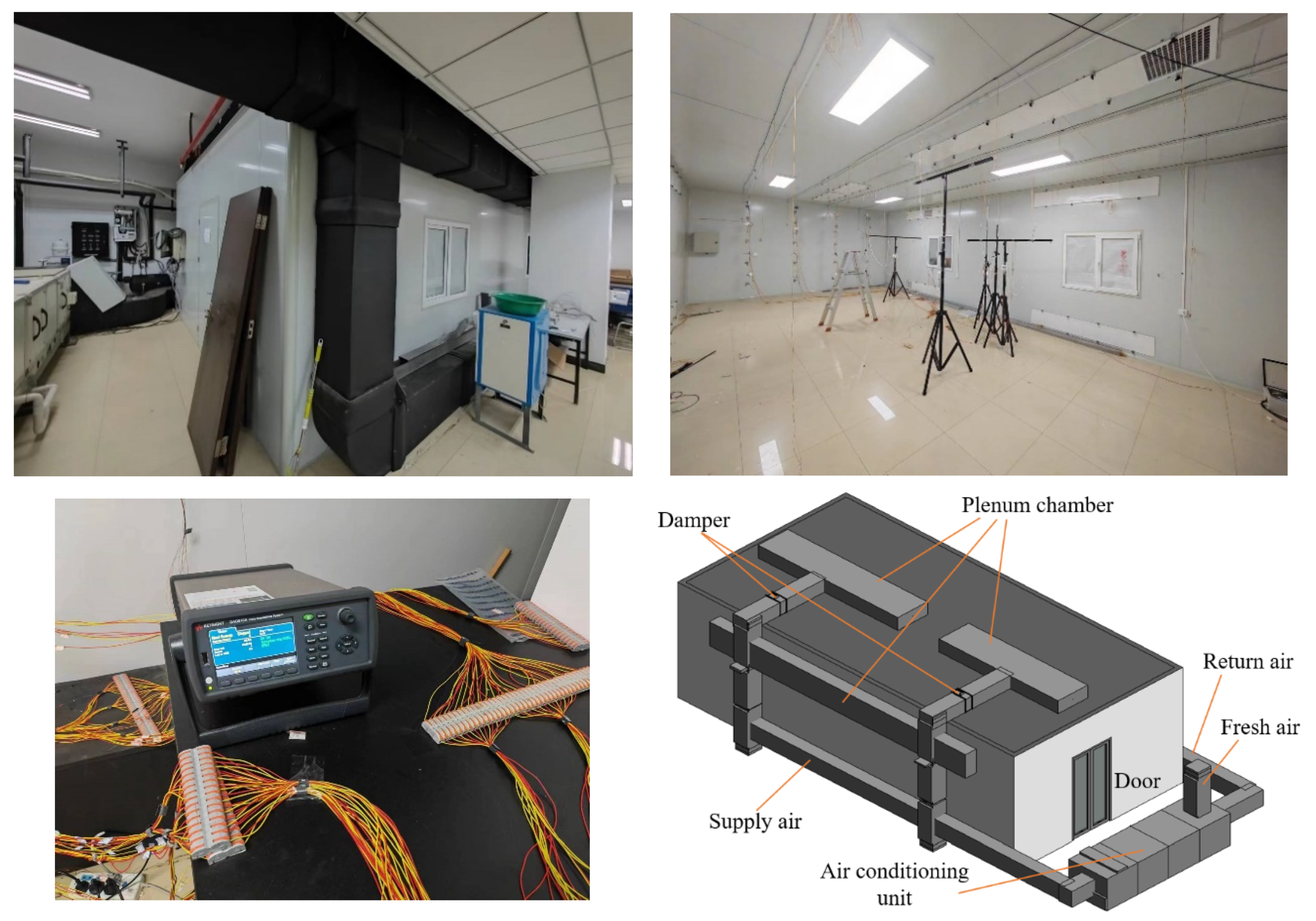
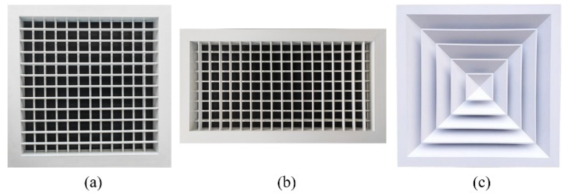
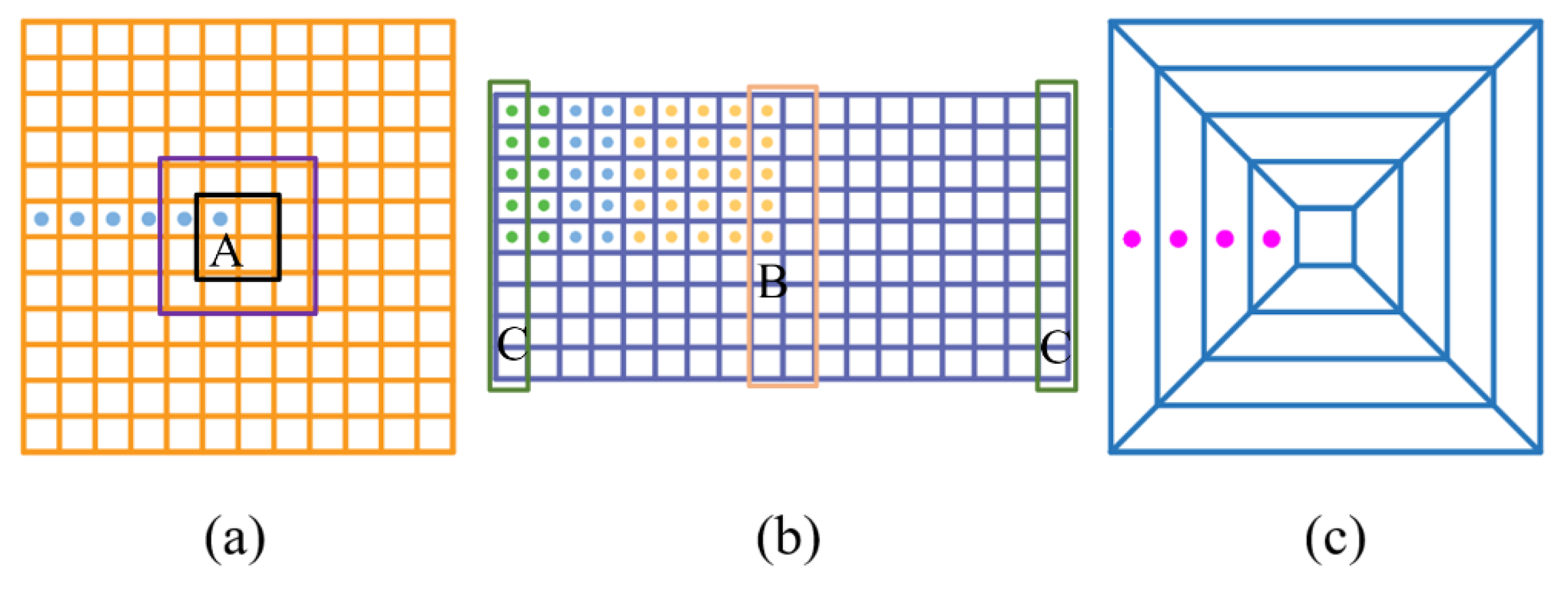
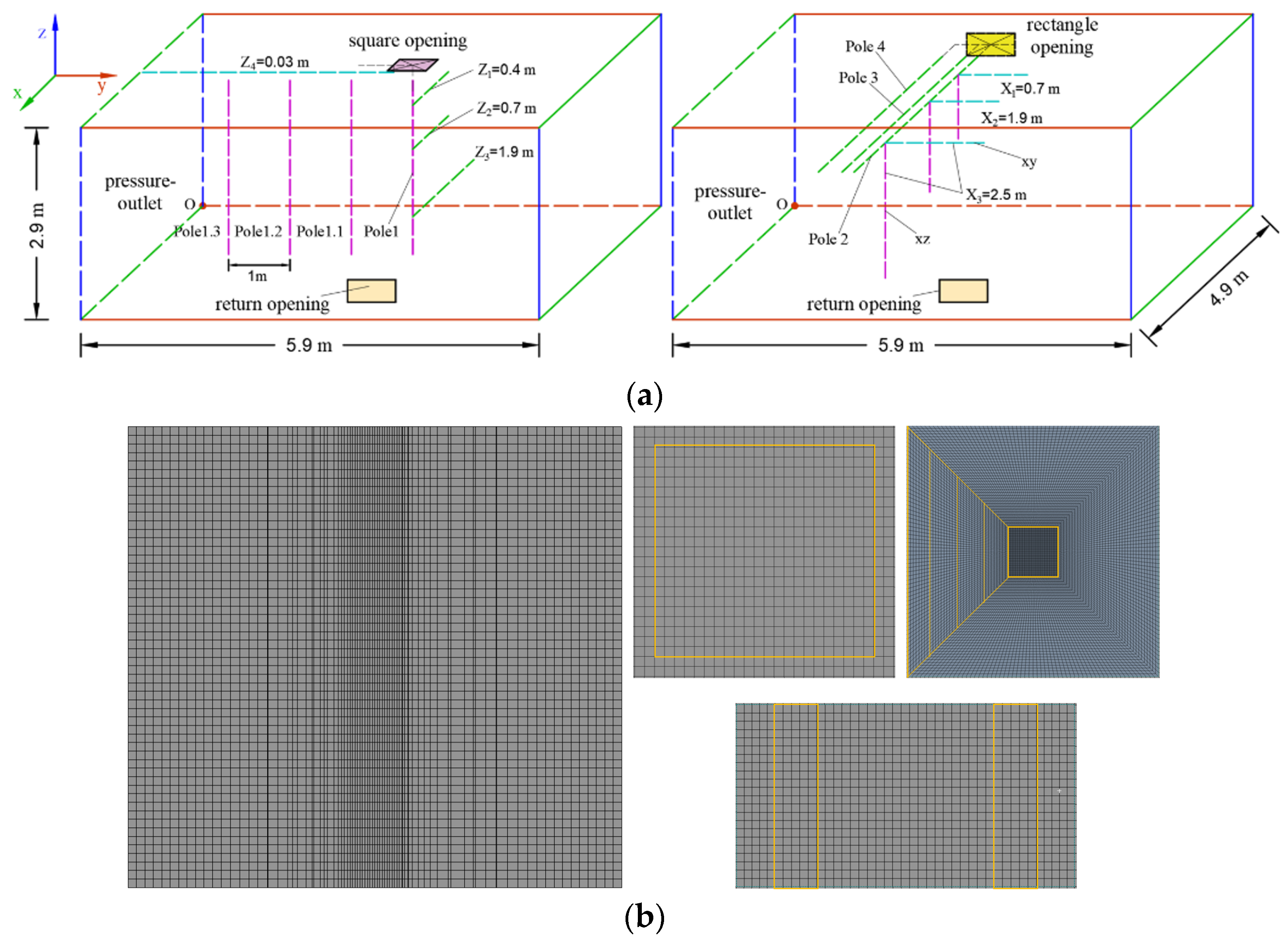
3.1. Experimental Setup
3.2. Experimental Procedure
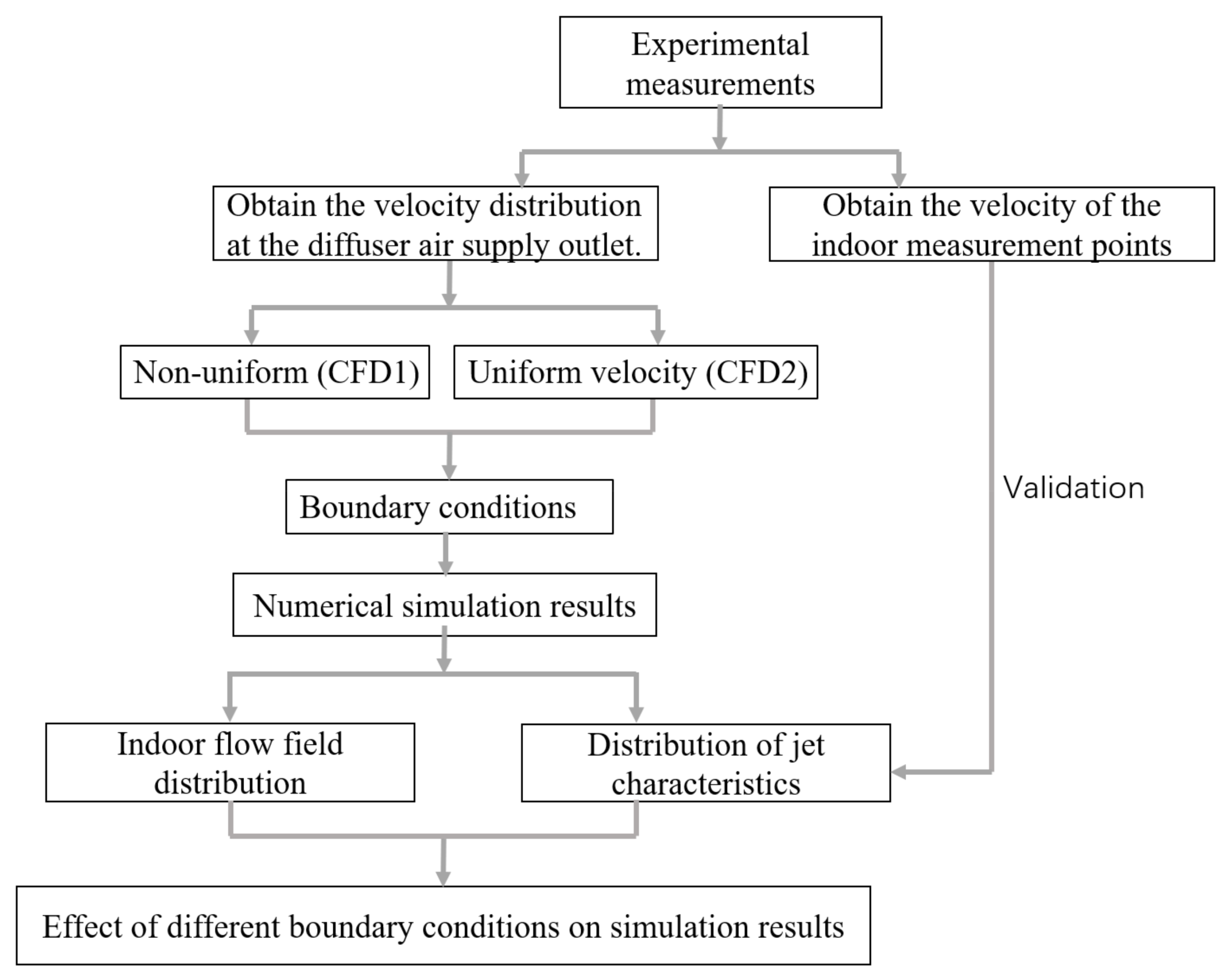
4. Numerical Model
5. Results and Discussion
5.1. Determination of Final Inlet Boundary Conditions
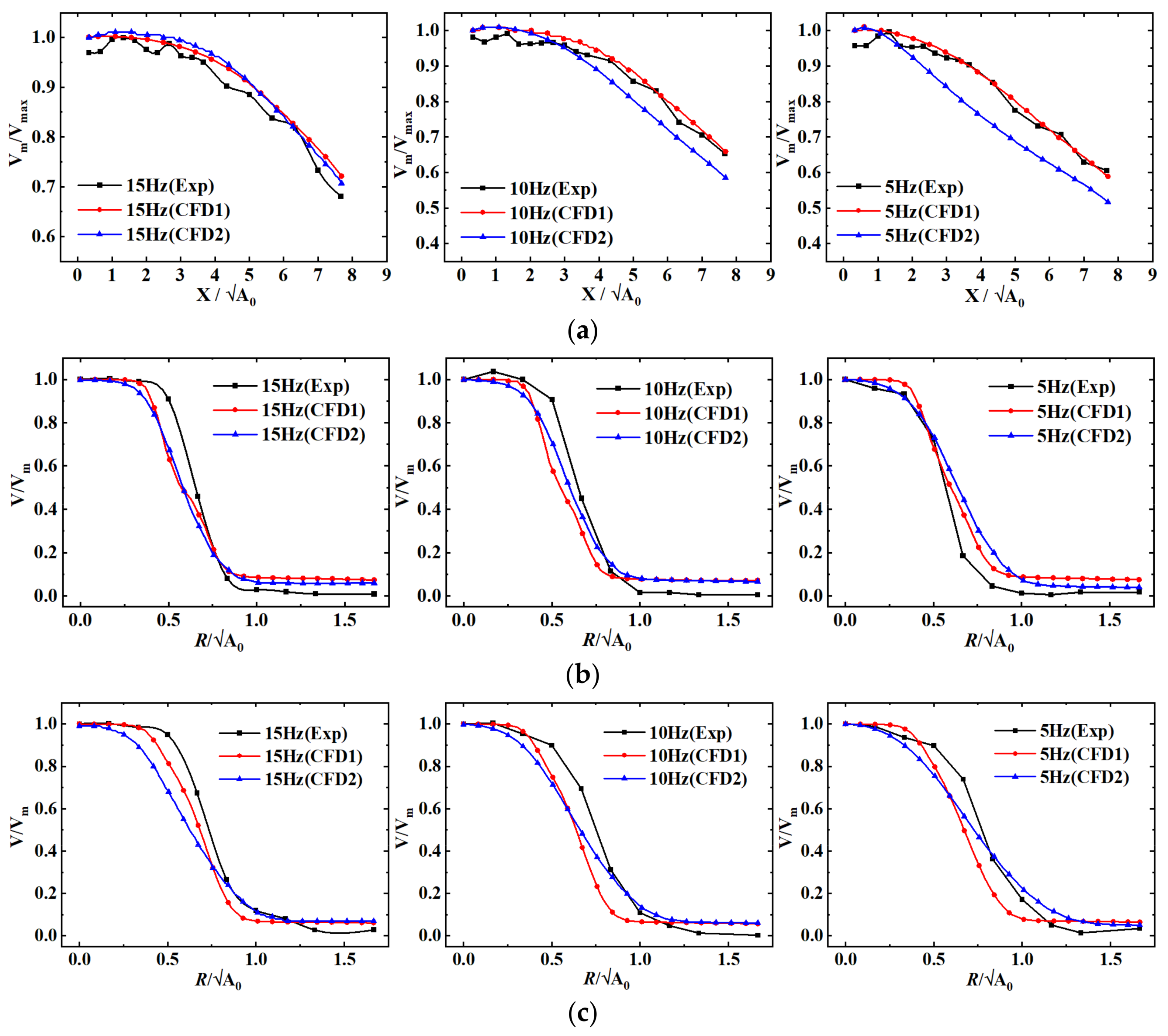
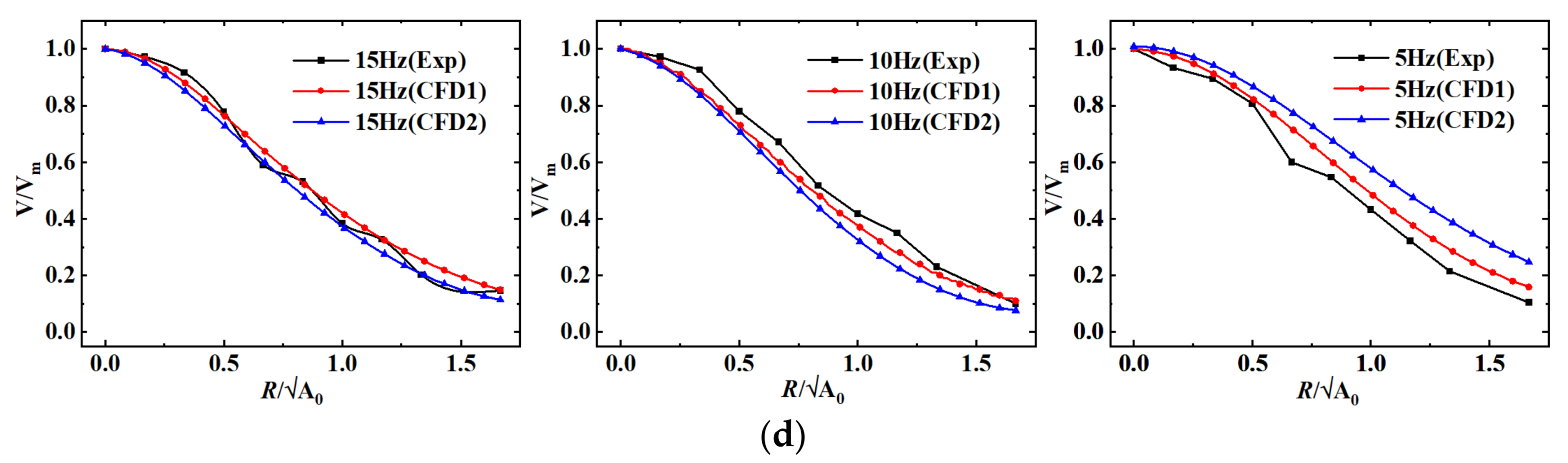
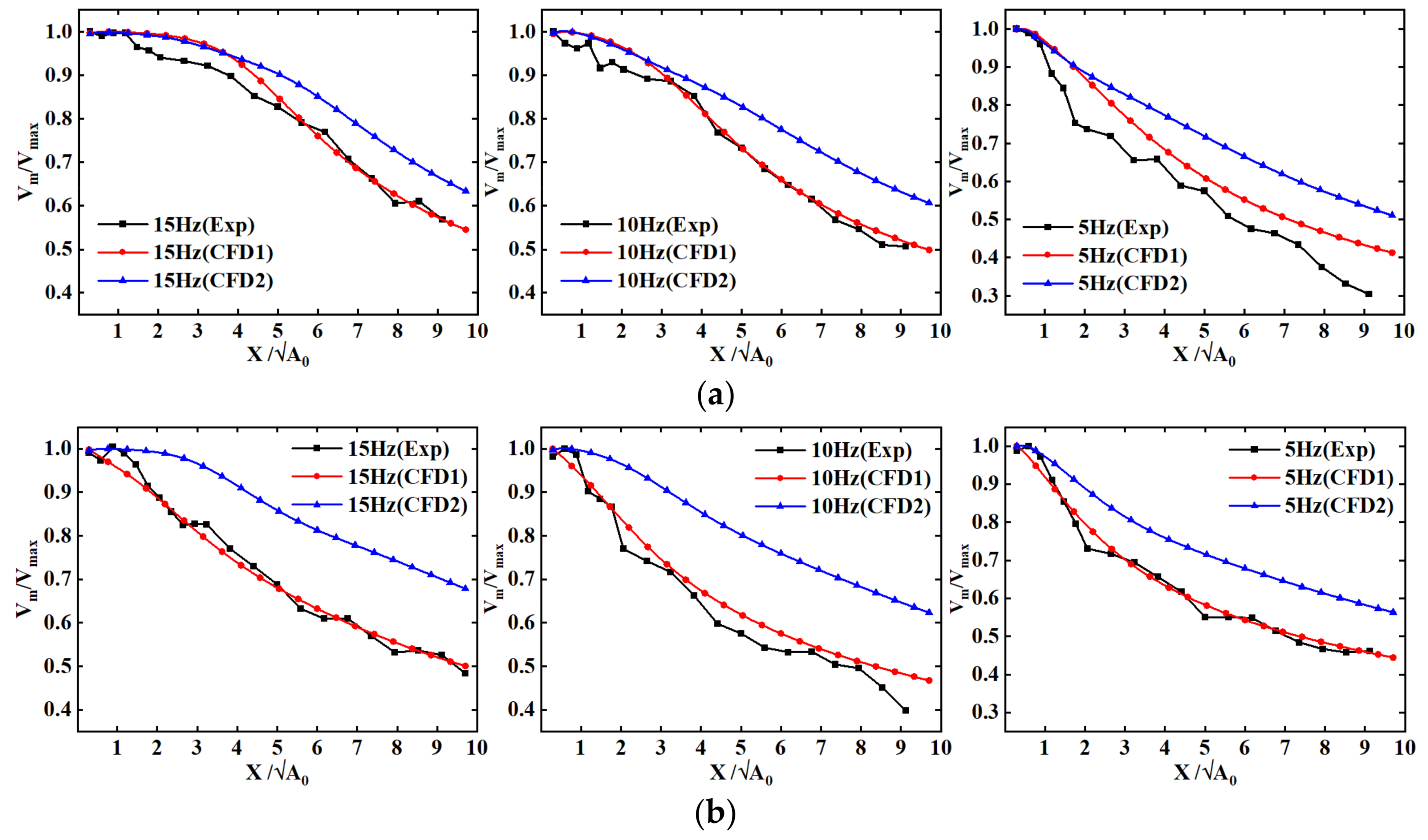
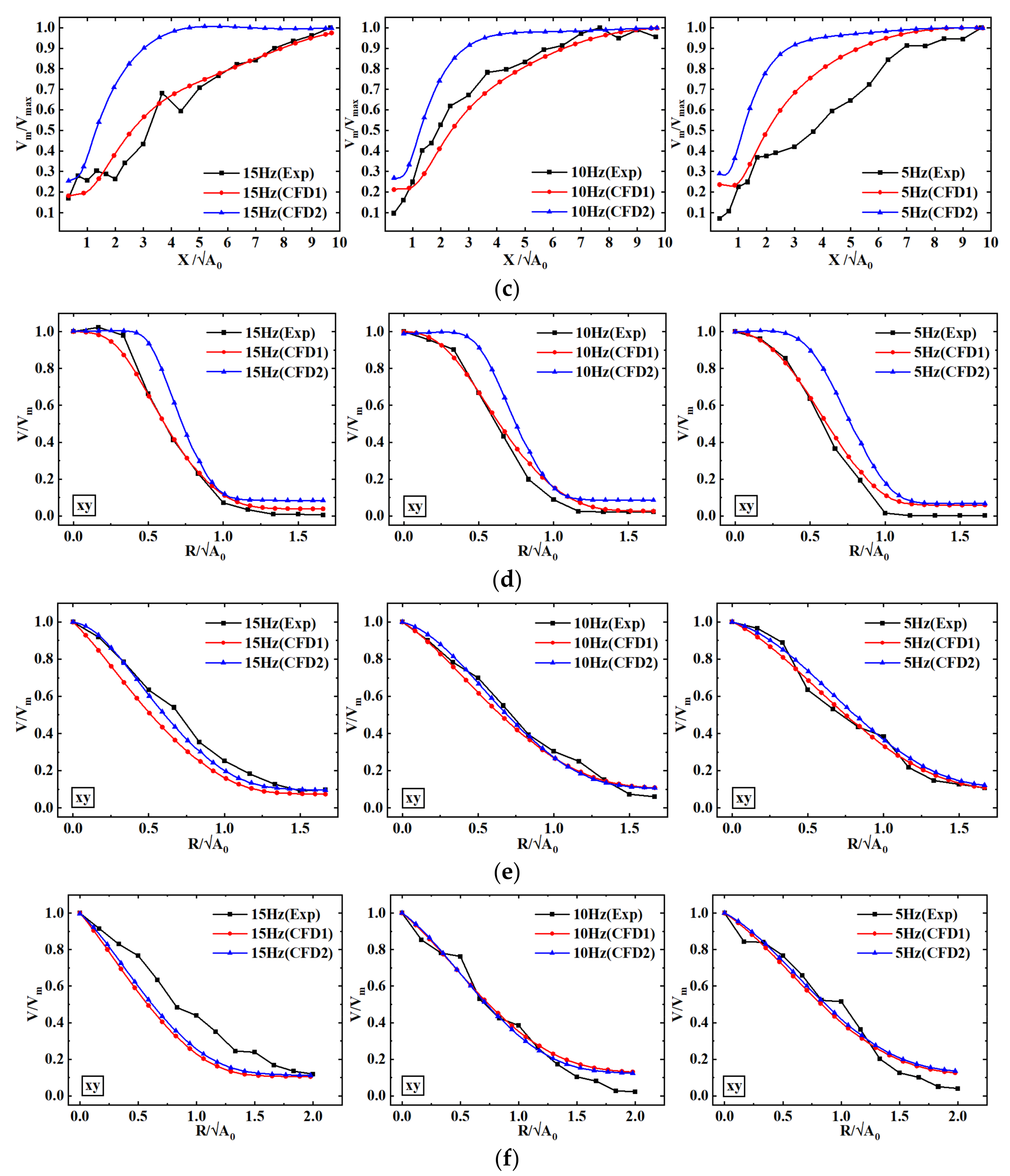
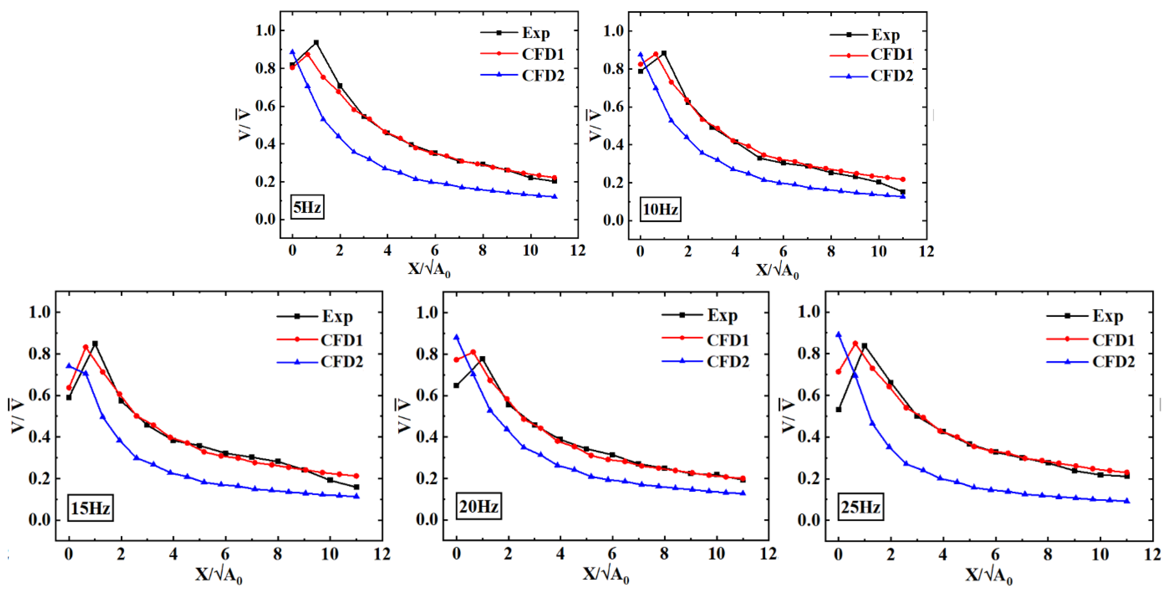
5.2. Effect of Two Types of Boundary Conditions on Jet Characteristics
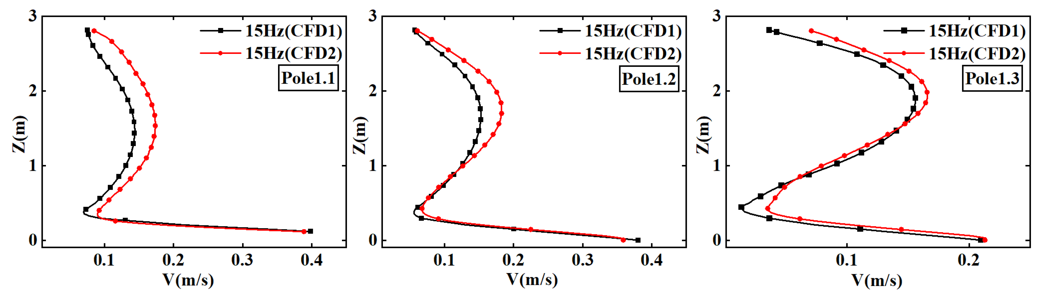
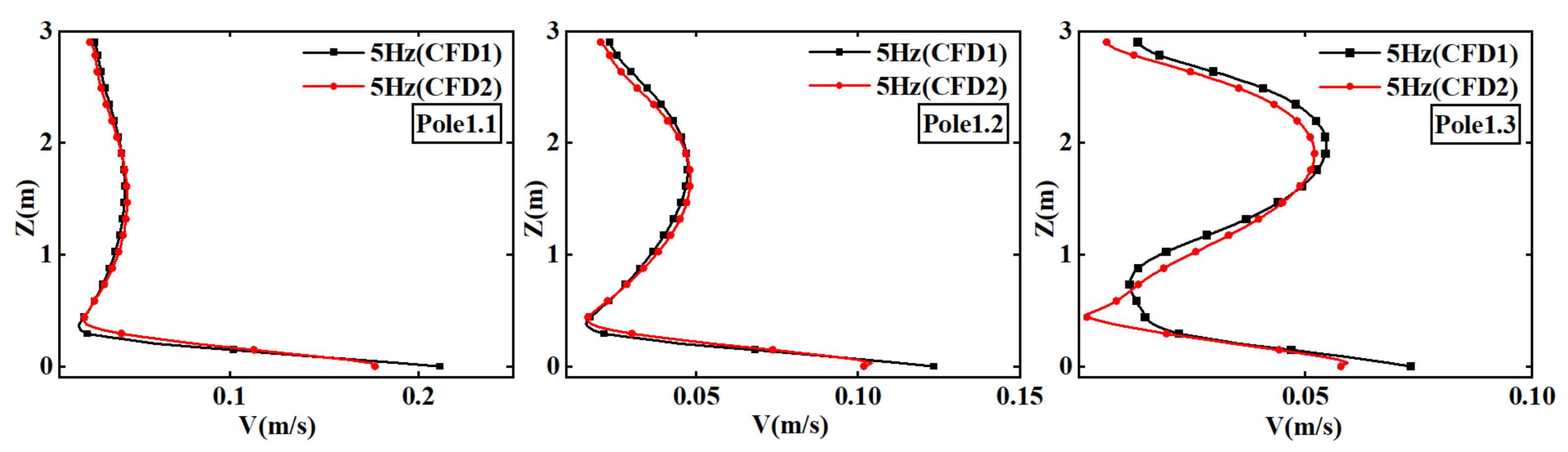
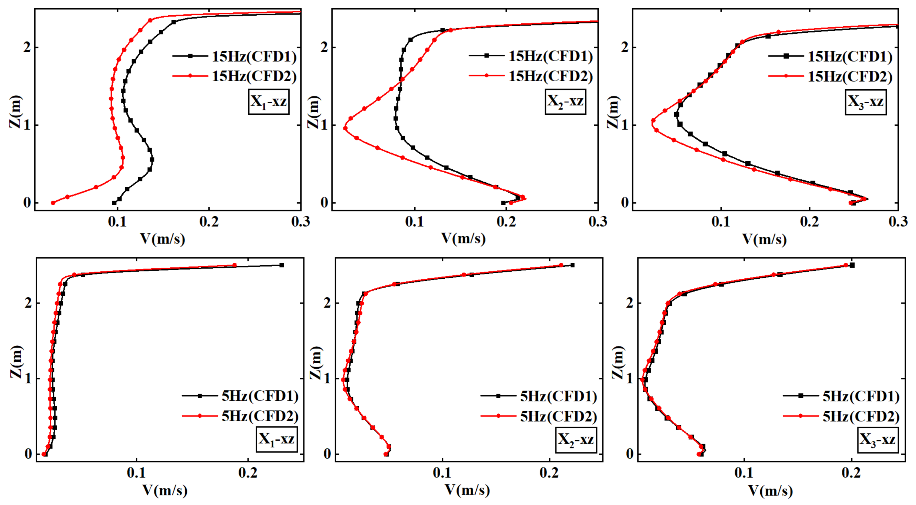
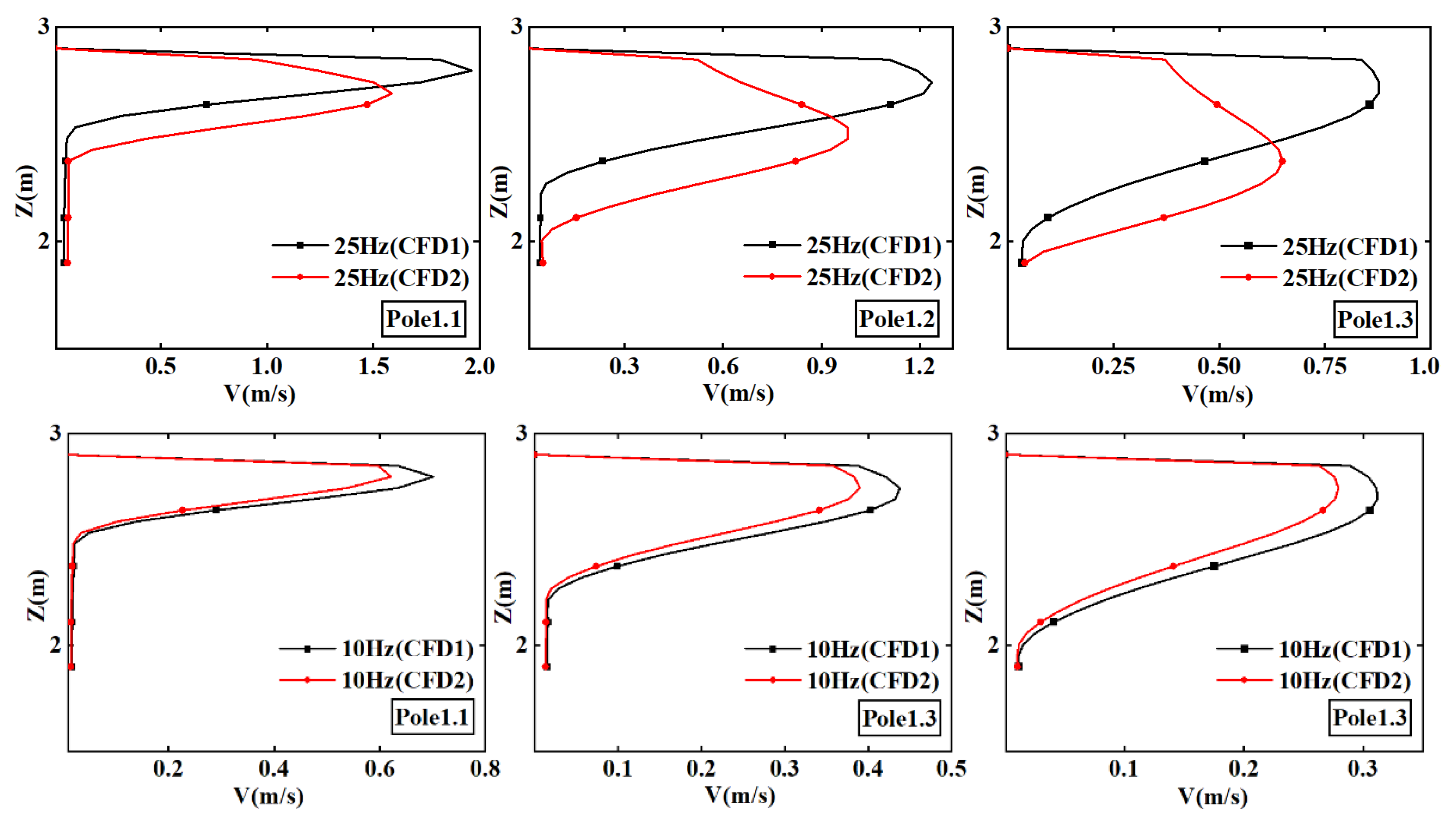
5.3. Effect of Two Types of Boundary Conditions on Indoor Flow Field
6. Conclusions
- 1
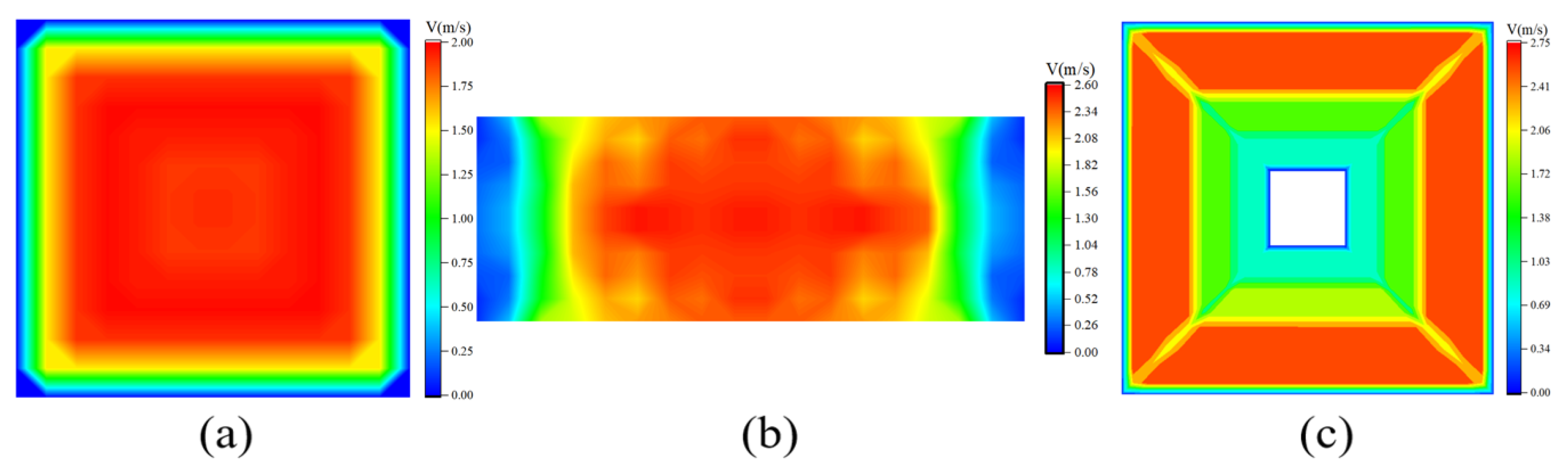
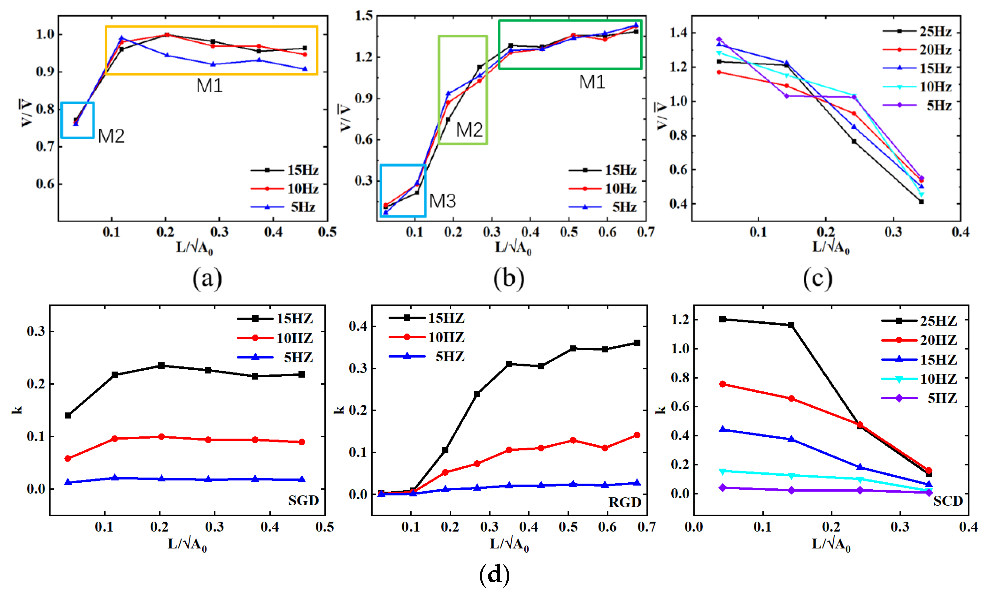
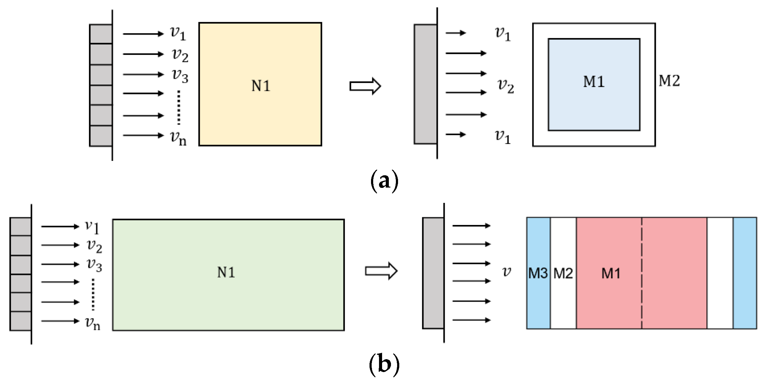
- For grid diffusers, the aspect ratio affects the distribution of the outflow velocity from the diffuser. When the aspect ratio of the grid diffuser is greater than 2, the velocity distribution in the width direction can be considered uniform. For ceiling diffusers, the velocity distribution monotonically decreases from the edge of the diffuser to the center of the diffuser.
- 2
- When the aspect ratio is 1 and the average outflow velocity exceeds 1.83 m/s, the effect of the non-uniformity of the outflow velocity of the grid diffuser on the jet characteristics does not exceed 5%. Furthermore, the use of uniform velocity as the velocity-inlet boundary condition will result in at least a 14.2% error. Because underfloor air supply usually sends air directly into the room at low air velocity, it is particularly important to consider the uniformity of the outflow velocity.
- 3
- When the average air velocity of the air supply outlet is greater than 2.0 m/s, the error brought by the non-uniform outflow velocity to the indoor flow field must be considered.
Author Contributions
Funding
Data Availability Statement
Conflicts of Interest
Nomenclature
| A | Area (m2) |
| A0 | Gross area of the diffuser (m2) |
| L | Distance from the edge of the diffuser (m) |
| R | Radial distance of the point from the centerline of the jet (m) |
| RGD | Rectangle grille diffuser |
| SCD | Square ceiling diffuser |
| SGD | Square grille diffuser |
| Source term | |
| Vm | Centerline velocity (m/s) |
| X | Distance from diffuser (m) |
| Effective diffusion coefficient | |
| m | Mass flow rates (kg/s) |
| k | Turbulent kinetic energy |
| q | Heat flux (W/m2) |
| t | Time |
| x,y,z | Co-ordinate system |
| ρ | Air density (kg/m3) |
| Subscripts | |
| in | Simple opening inlet conditions |
| r | Real conditions |
| max | Maximum |
References
- Zhu, H.-C.; Cao, S.-J. Fast prediction for multi-parameters (concentration, temperature and humidity) of indoor environment towards the online control of HVAC system. In Building Simulation; Tsinghua University Press: Beijing, China, 2020; Volume 14. [Google Scholar]
- Yau, Y.; Poh, K.; Badarudin, A. A numerical airflow pattern study of a floor swirl diffuser for UFAD system. Energy Build. 2018, 158, 525–535. [Google Scholar] [CrossRef]
- Dang, Y.; Luo, X.; Chang, B.; Huang, X.; Feng, Z.; Gu, Z. Local attachment ventilation system for the unearthed relic preservation area within site museum. Sustain. Cities Soc. 2022, 77, 103537. [Google Scholar] [CrossRef]
- ISO 7730:2005; Ergonomics of the Thermal Environment—Analytical Determination and Interpretation of Thermal Comfort Using Calculation of the PMV and PPD Indices and Local Thermal Comfort Criteria. International Organization for Standardization: Geneva, Switzerland, 2006.
- ANSI/ASHRAE Standard 55-2004; Thermal Environmental Conditions for Human Occupancy. American Society of Heating, Refrigerating and Air-Conditioning Engineers, Inc.: Atlanta, GA, USA, 2004.
- Alfano, F.R.A.; Olesen, B.W.; Palella, B.I.; Riccio, G. Thermal comfort: Design and assessment for energy saving. Energy Build. 2014, 81, 326–336. [Google Scholar] [CrossRef]
- Varodompun, N. HVAC Ventilation Strategies: The Contribution for Thermal Comfort, Energy Efficiency, and Indoor Air Quality. J. Green Build. 2007, 2, 131–150. [Google Scholar] [CrossRef]
- American Society of Heating Refrigerating and Air-Conditioning Engineers, Inc. ASHRAE Handbook—Heating, Ventilating, and Air-Conditioning Applications, SI ed.; American Society of Heating Refrigerating and Air-Conditioning Engineers, Inc.: Washington, DC, USA, 2015. [Google Scholar]
- Halibart, J.; Zwolińska, K.; Borowski, M.; Jaszczur, M. Analysis of the Velocity Distribution in the Plenum Box with Various Entries. Energies 2021, 14, 3630. [Google Scholar] [CrossRef]
- Li, A.; Yang, C.; Tong, R.; Bao, X.; Qin, E.; Gao, R. PIV experiment and evaluation of air flow performance of swirl diffuser mounted on the floor. Energy Build. 2017, 156, 58–69. [Google Scholar] [CrossRef]
- Hurnik, M.; Kaczmarczyk, J.; Popiolek, Z. Study of Radial Wall Jets from Ceiling Diffusers at Variable Air Volume. Energies 2021, 14, 240. [Google Scholar] [CrossRef]
- Jun, L. Research and Application of Air Supply Opening Models in CFD Simulation; Southwest Jiaotong University: Chengdu, China, 2012. [Google Scholar]
- Nielsen, P. Description of Supply Openings in Numerical Models for Room Air Distribution. Ashre Trans. Symp. 1991, 98, 26. [Google Scholar]
- Hu, S.C. Airflow characteristics in the outlet region of a vortex room air diffuser. Build. Environ. 2003, 38, 553–561. [Google Scholar] [CrossRef]
- Topp, C.; Jensen, R.L.; Pedersen, D.N.; Nielsen, P.V. Validation of Boundary Conditions for CFD Simulations on Ventilated Rooms. In Proceedings of the 4th International Conference on Indoor Air Quality, Ventlation & Energy Conservation in Buildings, iAQVEC 2001, Changsha, China, 2–5 October 2001. [Google Scholar]
- Huo, Y.; Haghighat, F.; Zhang, J.S.; Shaw, C.Y. A systematic approach to describe the air terminal device in CFD simulation for room air distribution analysis. Build. Environ. 2000, 35, 563–576. [Google Scholar] [CrossRef]
- Nielsen, P.V.; Restivo, A.; Whitelaw, J.H. The velocitycharacteristics of ventilated rooms. Trans ASME J. Fluids Eng. 1978, 100, 291–298. [Google Scholar] [CrossRef]
- Gosman, A.D.; Nielsen, P.V.; Restivo, A.; Whitelaw, J.H. The Flow Properties of Rooms with Small Ventilation Openings. Trans. Asme 1980, 102, 316–323. [Google Scholar] [CrossRef]
- Srebric, J.; Chen, D.Q. A Method of Test to Obtain Diffuser Data for CFD Modeling of Room Airflow (RP1009). ASHRAE Trans. 2001, 107, 108–116. [Google Scholar]
- Xu, H.T.; Niu, J.L. A new method of CFD simulation of airflow characteristics of swirling floor diffusers. Proc Build. Simul. 2003, 3, 1429–1434. [Google Scholar]
- Huo, Y.; Zhang, J.S.; Shaw, C.Y.; Haghighat, F. A New method to describe the diffuser boundary conditions in CFD simulation. Indoor Air 1996, 96, 233–240. [Google Scholar]
- Zhang, T.; Lee, K.; Chen, Q. A simplified approach to describe complex diffusers in displacement ventilation for CFD simulations. Indoor Air 2009, 19, 255–267. [Google Scholar] [CrossRef]
- Heikkinen, J. Modelling of a supply air terminal for room air flow simulation. In Proceedings of the Air Movement &Ventilation Control within Buildings, Ottawa, ON, Canada, 24–27 September 1991. [Google Scholar]
- Chen, Q.; Moser, A. Simulation of a multiple-nozzle diffuser. In Proceedings of the 12th ATVC Conference on Air Movement and Ventilation Control within Buildings, The TEA AirInfiltration and Ventilation Centre, Ottawa, ON, Canada, 24–27 September 1991; Volume 2, pp. 1–13. [Google Scholar]
- Deng, B.; Zhang, Y.; Long, F. A superficial density method to describe the diffuser boundary condition in CFD simulation of indoor airflow. Build. Environ. 2018, 135, 280–285. [Google Scholar] [CrossRef]
- Cehlin, M.; Moshfegh, B. Numerical modeling of a complex diffuser in a room with displacement ventilation. Build. Environ. 2010, 45, 2240–2252. [Google Scholar] [CrossRef]
- Skovgaard, M. Turbulent Flow in Rooms Ventilated by Mixing Principle: Comparision between Computational Fluid Dynamics and Full-Scale Experiments. Ph.D. Thesis, Department of Building Technology and Structural Engineering, Aalborg University, Aalborg, Denmark, 1991. Indoor Environmental Technology Vol. R9145 No. [Google Scholar]
- Emvin, P.; Davidson, L. Numerical comparison of three inlet approximations of the diffuser in case E1 Annex20. In Proceedings of the 5th International Conference on Air Distributions in Rooms ROOMVENT ’96, Yokohama, Japan, 17–19 July 1996; Volume 1, pp. 219–226. [Google Scholar]
- Chen, Q.; Suter, P.; Moser, A. Influence of air supply parameters on indoor air diffusion. Build. Environ. 1991, 26, 417–431. [Google Scholar] [CrossRef]
- Lai, J.C.S.; Nasr, A. Two parallel plane jets: Comparison of the performance of three turbulence models. Proc. Inst. Mech. Eng. Part G J. Aerosp. Eng. 2005, 212, 379–391. [Google Scholar] [CrossRef]
- Deng, B.; Wang, J.; Tang, J.; Gao, J. Improvement of the momentum method as the diffuser boundary condition in CFD simulation of indoor airflow: Discretization viewpoint. Build. Environ. 2018, 141, 55–60. [Google Scholar] [CrossRef]
- Zhao, B.; Li, X.; Yan, Q. A simplified system for indoor airflow simulation. Build. Environ. 2003, 38, 543–552. [Google Scholar] [CrossRef]
- Abdelmaksoud, W.A. Simplified CFD Model for Perforated Tile with Distorted Outflow. Fluids 2022, 7, 112. [Google Scholar] [CrossRef]
- Abdelmaksoud, W.A. Experimental and Numerical Investigations of the Thermal Environment in Air-Cooled Data Centers. Ph.D. Thesis, Department of Mechanical and Aerospace Engineering, Syracuse University, Syracuse, NY, USA, 2012. [Google Scholar]
- Iyengar, M.; Schmidt, R.R.; Hamann, H.; VanGilder, J. Comparison between Numerical and Experimental Temperature Distributions in a Small Data Center Test Cell. In Proceedings of the ASME 2007 InterPACK Conference, Vancouver, BC, Canada, 8–12 July 2007; pp. 819–826. [Google Scholar]
- Kuznik, F.; Rusaoueen, G.; Brau, J. Experimental and numerical study of a full scale ventilated enclosure: Comparison of four two equations closure turbulence models. Build. Environ. 2007, 42, 1043–1053. [Google Scholar] [CrossRef]
- Ma, Z.; Xu, M.; Luan, J.; Liu, X.; Zhao, F. Statistical properties of turbulent free jets issuing from rectangular nozzles with different aspect ratios. J. Exp. Fluid Mech. 2017, 31, 54–61. [Google Scholar]


| Model | Range | Accuracy | Resolution |
|---|---|---|---|
| CTV114 | 0~2 m/s | ±3% of reading ±0.05 m/s | 0.01 m/s |
| CTV115 | 0~15 m/s | ±3% of reading ±0.2 m/s | 0.1 m/s |
| Case | CFD1 | CFD2 | ||||||
|---|---|---|---|---|---|---|---|---|
| Diffuser | SGD | RGD | SGD | RGD | ||||
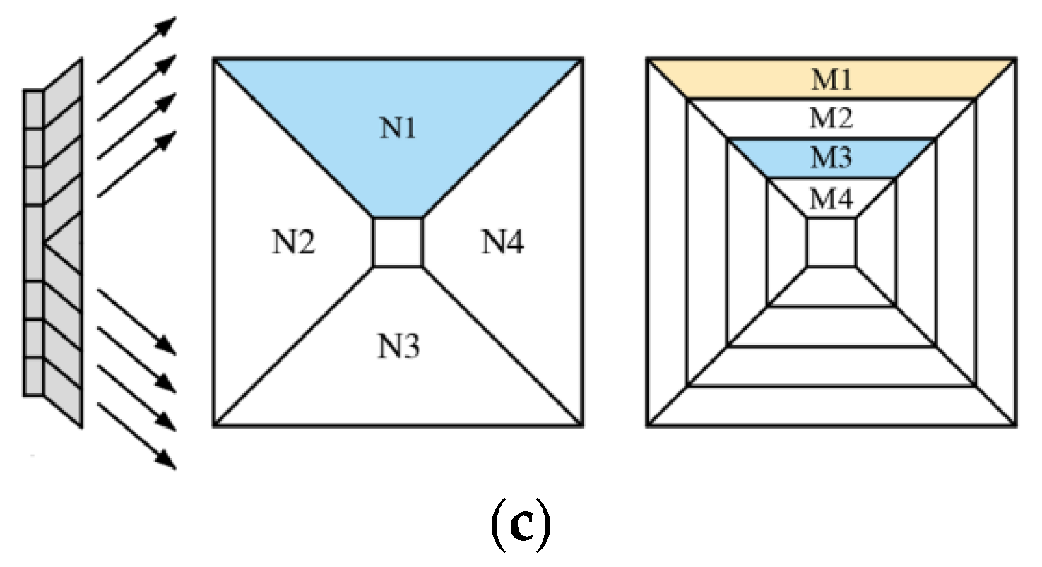
| Zone | M1 | M2 | M1 | M2 | M3 | N1 | N1 | |
| Velocity (m/s) | 15 Hz | 1.92 | 1.53 | 1.84 | 2.04 | 1.38 | 1.83 | 1.85 |
| 10 Hz | 1.25 | 0.98 | 1.42 | 1.58 | 0.77 | 1.19 | 1.08 | |
| 5 Hz | 0.56 | 0.45 | 0.67 | 0.71 | 0.42 | 0.54 | 0.47 | |
| Case | CFD1 | CFD2 | ||||
|---|---|---|---|---|---|---|
| Zone | M1 | M2 | M3 | M4 | N1 N4 | |
| Velocity (m/s) | 25 Hz | 4.48 | 4.4 | 2.78 | 1.5 | 3.64 |
| 20 Hz | 3.55 | 3.31 | 2.82 | 1.63 | 3.03 | |
| 15 Hz | 2.71 | 2.5 | 1.74 | 1.02 | 2.18 | |
| 10 Hz | 1.62 | 1.45 | 1.3 | 0.58 | 1.34 | |
| 5 Hz | 0.82 | 0.62 | 0.62 | 0.33 | 0.65 | |
Disclaimer/Publisher’s Note: The statements, opinions and data contained in all publications are solely those of the individual author(s) and contributor(s) and not of MDPI and/or the editor(s). MDPI and/or the editor(s) disclaim responsibility for any injury to people or property resulting from any ideas, methods, instructions or products referred to in the content. |
© 2023 by the authors. Licensee MDPI, Basel, Switzerland. This article is an open access article distributed under the terms and conditions of the Creative Commons Attribution (CC BY) license (https://creativecommons.org/licenses/by/4.0/).
Share and Cite
Li, K.; Song, L.; Zhang, X.; Wang, Q.; Hua, J. Study of Influence of Boundary Condition of Diffuser with Non-Uniform Velocity on the Jet Characteristics and Indoor Flow Field. Energies 2023, 16, 1079. https://doi.org/10.3390/en16031079
Li K, Song L, Zhang X, Wang Q, Hua J. Study of Influence of Boundary Condition of Diffuser with Non-Uniform Velocity on the Jet Characteristics and Indoor Flow Field. Energies. 2023; 16(3):1079. https://doi.org/10.3390/en16031079
Chicago/Turabian StyleLi, Kaijun, Linye Song, Xinghui Zhang, Qi Wang, and Jing Hua. 2023. "Study of Influence of Boundary Condition of Diffuser with Non-Uniform Velocity on the Jet Characteristics and Indoor Flow Field" Energies 16, no. 3: 1079. https://doi.org/10.3390/en16031079