

Forecasting the Monash Microgrid for the IEEE-CIS Technical Challenge †

School of Information Technology and Electrical Engineering, University of Queensland, St Lucia 4072, Australia
†
This paper is an extended version of our paper published in the 32nd Australasian Universities Power Engineering Conference, AUPEC 2022, 26–28 September 2022, Adelaide, Australia.
Energies 2023, 16(3), 1050; https://doi.org/10.3390/en16031050
Submission received: 24 November 2022
/
Revised: 10 January 2023
/
Accepted: 12 January 2023
/
Published: 18 January 2023
(This article belongs to the Topic Solar and Wind Power and Energy Forecasting)
Abstract
:Effective operation of a microgrid depends critically on accurate forecasting of its components. Recently, internet forecasting competitions have been used to determine the best methods for energy forecasting, with some competitions having a special focus on microgrids and COVID-19 energy-use forecasting. This paper describes forecasting for the IEEE Computational Intelligence Society 3rd Technical Challenge, which required predicting solar and building loads of a microgrid system at Monash University for the month of November 2020. The forecast achieved the lowest error rate in the competition. We review the literature on recent energy forecasting competitions and metrics and explain how the solution drew from top-ranked solutions in previous energy forecasting competitions such as the Global Energy Forecasting Competition series. The techniques can be reapplied in other forecasting endeavours, while approaches to some of the time-series forecasting are more ad hoc and specific to the competition. Novel thresholding approaches were used to improve the quality of the input data. As the training and evaluation phase of the challenge occurred during COVID-19 lockdown and reopening, the building demand was subject to pandemic-related effects. Finally, we assess other data sources which would have improved the model forecast skill such as data from different numerical weather prediction (NWP) models, solar observations, and high-resolution price and demand data in the vicinity of the campus.
1. Introduction
The efficient operation of a microgrid requires accurate energy forecasting and effective optimisation. This is referred to as the “predict + optimise” problem [1].
The same principles apply to the forecasting and optimisation of larger grids. New microgrids often operate entirely on renewable energy, and the modelling of such grids provides important lessons for the operation of national grids where rapid decarbonisation must occur. In this paper, we study a particular microgrid with a collection of buildings, associated solar panels and batteries.
Studying such a problem deeply and investigating which approaches worked best, and conducting a review of possible data sources can help many parties, such as forecasters, grid operators, and future competition organizers. In the last decade, several competitions have been organized, covering both the narrow forecasting-only problem and the larger “predict + optimise” problem.
Here, we describe the approach used in a competition to model the Monash University Microgrid, focussing on the forecasting aspect of the problem. In 2021, the IEEE Computational Intelligence Society ran a “predict + optimise” competition from 1 July to 3 November online [2].
The geographical context of the competition was in the city of Melbourne, in the state of Victoria, Australia. In this microgrid, the electricity demand at a set of six buildings is met by a set of six solar installations, while a set of batteries with differing capacities and efficiency rates may be charged or discharged to meet requirements. A related optimisation problem in the competition concerned how the energy requirements could be met at lowest cost using the batteries and foreknowledge of electricity prices.
The competition ran in two phases. In Phase 1 from 1 July to 11 October 2021, competitors were able to upload forecasts to a public “leaderboard” which would calculate the Mean Absolute Scaled Error (MASE) [3] of each the 12 time series for October 2020. The mean of these 12 MASE values would then be displayed on the leaderboard. At the end of Phase 1, the load and solar data of October 2020 (the 12 time series) was made public, and Phase 2, based on forecasting the month of November 2020, began.
From 13 October to 3 November 2021, competitors could upload forecasts, but the leaderboard only provided an indication of whether forecasts were better, worse, or the same as a reference forecast of all zero values. On 3 November the MASE and energy cost figures were released, while the energy data were released on 6 December 2021.
In this paper, we present the approach used to win the forecasting section of the competition, and describe the novel contributions (for example, thresholding and combining daily and hourly input data) which led to the model outperformance. We explain how the competition fits in the context of energy-forecasting competitions, in particular with reference to COVID-19 effects, and investigate how other data sources could have improved the results.
We review the recent literature relevant to the competition in Section 2. Section 3 describes the data available in the competition, a naive forecast, and the general approach used; Section 4 examines the specific case study of the competition, and Section 5 provides the results. Section 6 is a “post-mortem” discussion of what other predictor variables may be useful in this kind of forecasting, with implications, and Section 7 concludes the paper.
2. Literature Review
We consider literature from well-known energy forecasting competitions (largely the GEFCOM series and Kaggle-based competitions), other energy-forecasting ideas from the literature, and concerning energy usage and forecasting during COVID-19. These competitions are relevant as techniques specific to some of them could be applied to the competition described here.
2.1. Energy-Forecasting Competitions and Principles
To develop an accurate forecast for a specific case such as the microgrid under consideration, it is important to review past competitions and derive lessons from them. The Global Energy-Forecasting Competition (GEFCOM) has been run three times (2012, 2014 and 2017) with themes of forecasting electricity load, solar, wind and price, with both point and quantile forecasting.
The 2014 and 2017 iterations of GEFCOM [4,5] provided strong evidence that random forests were one of the most successful techniques in energy forecasting (or at least in related competitions). For example, in the solar track of GEFCOM 2014, three of the top five entries used quantile regression forests or random forests as part of the model. In the GEFCOM 2017 competition for hierarchical load forecasting, three of the top seven entries used quantile regression-based models. For the sake of saving time, we used quantile regression forests for both building and solar modelling.
Concerning GEFCOM 2012, Table 2 of [6] summarised the methods used in the hierarchical load forecasting track plus a “Vanilla Benchmark” using multiple linear regression (MLR). Linear regression is a simple method for relating weather and temporal variables to the output variable (load). Clearly, the relationship between input weather variables such as temperature and load is non-linear requiring transformation such as the use of heating and cooling degree days; and similarly for the time of day/Julian date temporal variables.
Ten methods were given, of which three used MLR or ensembles featuring MLR, three used neural networks, and one (Chaotic Experiments) used random forests. Data cleaning was a key challenge of the competition.
The winning team [7], used multiple linear regression, with key steps of combining models from multiple weather stations, outlier removal and public holiday treatments. A quadratic function was used to account for the non-linear relationship of temperature with load. A separate model was built for each zone and hour of the day. Then the temperature for each zone was modelled in terms of various weather station inputs and some holidays are treated as weekend days. Two tracks of the GEFCOM 2014 competition were particularly relevant, as they covered load and solar forecasting (GEFCom2014-L and GEFCom2014-S). The competition assessed probabilistic, rather than point forecasting. Additionally, the weather data provided was from ECMWF, as in the competition described in this paper.
The winning team in the load track [8] used a quantile generalized additive model to win the load and price forecasting tracks after testing random forests, gradient boosting machines and generalized additive models.
We considered generalized additive models for our work, but random forest models achieved better performance with little training required.
A quantile regression forest model was used by [9] as part of their approach; using all the ECMWF ERA5 variables provided, plus temporal variables: hour, day of year, and month.
The 2017 competition focussed on hierarchical probabilistic load forecasting; as in previous GEFCOM instances, quantile regression forests, gradient boosting machine, neural networks, multiple linear regression and various ensembles were used. However, the weather variables were not provided by ECMWF and so lessons cannot be applied directly here as for the 2014 instance. Of the solution papers, ref. [10] provided labelling ideas for each time series, which proved to be a useful concept for the IEEE challenge.
Another competition run on Kaggle was described in [11] using machine learning for solar forecasting. This was an early example of a competition using NWP data in the US (specifically, Oklahoma) for solar forecasting; gradient boosting regression trees were found to outperform other methods.
Other papers have focussed on forecasting day-ahead load and solar generation in large electricity markets using weather forecast data.
In the context of forecasting the Australian National Electricity Market [12] wrote about forecasting day-ahead electricity load. They used a heating/cooling degree day approach, with lagged and leading variables. Linear regression and piecewise linear modelling of temperature effects were used for a regional electricity forecast in Australia. The approach was refined in [13] to forecast quantiles. They noted that important factors for forecasting were the seasonality of load, temperature and special day effects. Lagged load effects were noted to be critically dependent on the day of the week.
A paper on solar forecasting [14] noted that the commonly used ensemble technique in wind and solar power forecasting was to blend weather data from different sources. This was important in the competition studied here, with some data hourly and other data available on a daily resolution.
Since the IEEE-CIS competition, papers from winners have appeared describing their forecasting and optimisation approaches [15,16,17,18,19,20,21]. Two competitors used LightGBM (gradient boosting machines), two used random forests or quantile regression forests, one used ResNet/Refined Motif, and two used ensemble approaches (one involved neural networks and the other random forests, gradient boosting machines, and regression). Further details may be found in [2] while the effect of different error metrics is examined in [22].
For the design of a forecasting competition, it is important to choose a correct error metric (in this competition, MASE or Mean Absolute Scaled Error) and to avoid using training data in the evaluation phase.
Forecast evaluation methods were examined in [23]. The authors discussed data leakage, where training data are used in the test or evaluation set. In the context of this competition, data partitioning was applied to retain the temporal order of the time series, splitting it across phases. Thus, the month of October 2020 was used in Phase 1 to allow competitors to refine their models while November 2020 was used in Phase 2 for the evaluation. A possible issue with non-stationarity occurred; that is, the “return to campus” effect observed in November 2020 had not been seen since the March 2020 lockdown.
In a similar manner to leakage, we discuss extra sources of data in Section 5 which could have been used as input data by the competition designers or by unethical competitors. In the GEFCOM competition run on Kaggle, the team which initially achieved the lowest score exploited “some external utility data” in their final submission [24].
The authors cite [25,26] as arguing that point forecast evaluation alone is insufficient for all end use cases. The second paper proposes assessing a range of point forecast error measures in competitions, in the context of discussing the results of the “M4” competition [27].
Figure 11 and Table 1 of the paper provide a large flowchart for point forecasting. For example, RMSE or “root mean squared error” and MAE/MASE or “mean absolute (scaled) error” are discussed. MAPE is inappropriate for time series containing zero values, such as solar time series used in the competition. Thus, it was appropriate for the multiple time series containing non-stationarities of the seasonality type, to choose MASE as a forecast metric.
MASE is calculated as defined in [3], as follows. Let , be the observations at time t and be the forecast at time t, with the forecast error . Then calculate the scaled forecast errors as
with MASE = mean().
A detailed study on the theory and practice of forecasting was published in [28]. In particular, one subsection (3.4.3) gives a summary of recent references based on the time horizon of the forecasts. It is noted that 15 min forecasts (as seen in the challenge) are classified as “VSTLF” (i.e., Very Short-Term Load Forecast) while in MTLF (medium-term load forecasts) one may forecast electrical peak load, which is relevant for the optimisation phase of the challenge. VSTLF is stated to require meteorological data and day type identification codes.
Recent systematic reviews of electricity load forecasting models have been provided in [29,30,31,32]. The paper [32] recommended extreme gradient boosting as a technique, studying Panama’s electricity load over the last 5.5 years, using temperature, humidity and temporal variables. Various other single approaches have been examined in other papers [33,34,35,36,37,38]. For example, deep neural networks, deep learning, combinations of stationary wavelet transforms, neural networks, hybrid models, PSO (particle swarm optimisation) and ensemble empirical mode decomposition were examined. An extensive review of ML methods for solar forecasting was given in [39], which noted that SVM, regression trees and random forests gave similar results and ensemble methods always outperformed simple predictors.
2.2. COVID-19 Energy Usage
During the period of COVID-19 since December 2019, there have been many papers published about the effect of “lockdowns” on energy use in buildings. More specifically, several papers have been published on energy use in universities in the UK, Spain, Malaysia and Australia explaining the effect of full and partial lockdowns and reopenings, and what kind of loads are running irrespective of whether a lockdown is in place. For a more general survey of how COVID-19 affected household energy usage in an Australian context, see [40].
One study [41] looked at 122 buildings in Griffith University, Australia. The buildings were across five campuses in the Gold Coast, Australia and compared the “COVID-19” year February 2020 to February 2021 to the “pre-COVID” year February 2019–February 2020. Learning and administration moved off campus while research remained on campus, saving 16% of energy year on year. Air-conditioning reduction accounted for half of the energy-use change. In agreement with [42] it was found that research buildings have highest energy-use intensity and academic offices the least. They noted that it was important to assess the special occupancy conditions of these buildings and not model them as regular commercial or residential buildings.
Some researchers required specialised equipment and could not work from home. The energy savings may have been caused by reduced hours of operating building equipment, such as HVAC (heating ventilation and air conditioning) which was shut down in some types of buildings. In the location of the university (with a sub-tropical climate) there was high demand for cooling in summer but little demand for heating in winter.
Examining the University of Almeria in Spain, ref. [43] found that the library category was most influenced by shutdowns and the research category was least influences. University campuses were noted to use energy in a different way from residential buildings, with differing occupancy rates, HVAC, lighting, computers and so on. UPS, fridges and freezers, security systems, exterior lighting and telecommunications could not be turned off and were characterized as “heavy plug load”. Thus, building by building modelling is appropriate, which was seen in the competition. Library, sport, and restaurant buildings were affected strongly at different times.
At the BarcelonaTech university campus [44] studied 83 buildings, identified the main use case for each, calculated heating and cooling temperature effects, and showed estimated occupancy. They again noted that research buildings experienced the least proportion of avoided energy use during lockdown. Further savings were not possible due to some buildings having a low level of centralised controls.
The study [45] examined a 7-level research complex building in Malaysia. They noted a strong weekend/weekday usage pattern with centralised air conditioning during work hours and studied the effects of partial and complete lockdowns.
In Scotland, ref. [46] examined public buildings during 2020 and 2021 in the context of “lockdown fatigue”. Library buildings were noted as offering higher EU (electricity use) and EUI (electricity use intensity) reduction potential.
In summary, the research on universities could not be directly applied to the competition as it was unknown which classification the buildings fell into. However, the choice of input data to the model (that is, the starting point chosen for each building’s data) had a large effect on the performance of the model.
A competition was organized by IEEE [47] requiring competitors to forecast day-ahead electricity use in March and April 2021 from a “metropolitan electric utility”. Four years of data and weather variables were supplied (historical and forecast). Out of 20 teams that finished the competition, only nine had a “significantly lower MAE” compared to the persistence-based benchmark load forecast. The persistence forecast set Sunday and Saturday load to the previous Sunday or Saturday; Monday and Tuesday to the previous Friday, and Wednesday to Friday from two days prior. The top teams used ensembles of models which were weighted based on the recent performance of individual models.
The competition organizers noted that multi-model approaches were dominant, and this dominance had also been noted in the recent M5 competition [48]. They concluded that the winning models were adaptable to sudden changes in conditions such as lockdowns, but that it was not clear if the models were robust or could be generalized to other circumstances.
The winning team published details of their approach in [49]. They used an ensemble of 72 models including linear regression, GAMs, random forests, and MLPs, using an “online robust aggregation of experts”. The aggregation method is more fully described at [50] in the context of lockdowns in France.
The third placed team [51] explained their approach involving cleaning of weather data using linear interpolation, lagged load effects, outlier detection and adjustment for holidays. Their ensemble of 674 models incorporated STL decomposition with exponential smoothing, an AR(P) time series model, GAMs, and regression models.
The organizers stressed that publication of the methods was critical to maximize benefit to society, in contrast with commercial data science competitions.
3. Materials and Methods
In this section, we describe the data provided by external sources and by the competition organizers. The external data consists of weather data from two different meteorological organizations and electricity price data from the grid operator in Australia.
We then provide a general description of the random forest algorithm, and give a baseline error rate based on various “naive” forecast approaches.
3.1. Prediction Data
Competitors in the challenge were permitted to use external data from two sources: the Australian Bureau of Meteorology (BOM) weather data available through manual download from Climate Data Online [52] and the European Centre for Medium-Range Weather Forecasts (ECMWF) [53,54] data provided by OikoLab [55]. Thus, the competitors were allowed to use “perfect forecast” weather data. From the BOM data, we used only the “daily global solar exposure” data, although daily minimum and maximum temperatures and daily rainfall data were available. The European Centre model is known as ERA5 and provides hourly historical weather (reanalysis) data.
The BOM “daily global solar exposure” data is measured from midnight to midnight each day, and is the total solar energy for a day falling on a horizontal surface. For the stations used in this study, values ranged from 1.3 to 32.3 MJ per square metre in 2019 and 2020. For the competition, these data were available at three nearby sites—Oakleigh, Olympic Park, and Moorabbin (BOM sites 86077, 86088 and 86338, respectively).
Table 1 lists and describes the variables used to model solar output in several recent papers and this competition: GEFCOM [4,56,57], PVLIB [58], and PVCompare [59]. The descriptions come from the ECMWF “GRIB Parameter Database” [60]. Their use in competitions is shown in Table 2.
One study [61] used the higher-resolution ERA5-Land data, which provides 0.1 degree grid resolution coverage of the Earth, and four of the “PVLIB” variables i.e., wind speed (u and v), surface solar radiation downward, and 2 m temperature.
The PVLIB source code [62] which derives values from the European Commission’s Photovoltaic Geographical Information System (PVGIS) [63] takes into account global horizontal irradiance, direct normal irradiance, diffuse horizontal irradiance, the plane of array irradiance (global, direct, sky diffuse, ground diffuse), solar elevation, air temperature, relative humidity, pressure, wind speed and direction. The PVGIS data is itself partially dependent on ECMWF data and the variables chosen are similar to those listed in Table 2.
3.2. Building and Solar Data
3.2.1. Solar
As a rule of thumb, a 4 kW system in Melbourne produced 14.4 kWh of solar energy daily, according to an estimate by Australia’s Clean Energy Council [64]. Equivalently, this can be expressed as a “capacity factor” of 15.0% relative to the size of the system. In the centre of Australia in Alice Springs, such systems can produce 20.0 kWh per year; that is, a capacity factor of 20.8%. This can also be expressed in a “kWh/kW” form—that is, 3.6 kWh/kW in Melbourne and 5 kWh/kW in Alice Springs.
The solar installations, named Solar0 to Solar5, appeared to be of sizes of approximately 8 to 50 kW. The data for Solar0 only began in April 2020, but the estimated capacity factors of each installation (using data up to and including October 2020) ranged from 15.9% (Solar5, max 40.4 kW) to 23.5% (Solar1, max 12.7 kW).
For Solar0, 86% of the time-series values are non-zero; for Solar5, this proportion is 30%; while for the others, the value ranges from 38% to 48%. It seemed that some kind of cleaning or thresholding approach could be used to improve performance for forecasting Solar0 and Solar5 values and this proved to be the case.
A Q-Q plot of the six solar installations, using all available data, is shown in Figure 1. The red line represents Solar1. On closer examination, the kink in this line was found to be caused by cumulative data in the Solar1 time series in late 2020. Thus, not all the data from Solar1 could be trusted or used without cleaning. We thresholded the data from Solar1, Solar2 and Solar3 time series to begin from 22 May 2020. All of the Solar0, Solar4 and Solar5 time series were used in training, although only hours where at least one period of generation (of four) was greater than 0.05 kW were used for Solar0 and Solar5 training.
3.2.2. Buildings
The provided data for the buildings and solar installations began at various dates, with the earliest data available from “Building 3” on 1 March 2016. The data for some buildings was very spotty; for example, Building 4 had 46,733 values but 18,946 of the values were unavailable. The modal and median value for Building 4 (19,621 occurrences) was 1 kW and all the other values were 2, 3, 4 or 5 kW. A perfect approach for data such as Building 4 would forecast one of these discrete values as the MASE of every series was significant for the competition, regardless of size.
We omitted one day in October 2020 from the building training data due to a state public holiday effect in the data (Friday before Grand Final). It was unclear whether the public holiday was influencing this day, while November 2020 (the evaluation month) had no significant public holidays.
3.3. Naive Forecasts
It is instructive to consider the performance of naive forecasts (for example, persistence-based or those based on median of each time series for the most recent month).
To develop a persistence-based forecast, we examined the building and solar traces for November 2019 versus previous data. (We also checked the time series for solar against previous time series reversed in case seasonality effects were useful). It was quickly determined that for November 2019, for a “month-ahead” forecast, the best lag period was 30 days (720 h) for the solar and 35 days (840 h) for the buildings, which preserved the weekend patterns. This was the lag period that generally minimized the sum of squares of differences, comparing November 2019 to previous time periods of the same length. The organizers explained that for computing the MASE, they used a 28-day-ahead seasonal naive forecast (i.e., 2688 15-min periods).
Applying this to the November 2020 forecast, we achieved a mean MASE over the 12 time series of 1.1754. The final leaderboard for Phase 2 contained 14 different forecasts for Phase 2, of which 10 had a lower MASE than this naive forecast.
Classifying each hour in the data by weekday/weekend type and by hour (i.e., 48 classifications) and setting each value for November 2020 to the median of the corresponding hourly/day type value for the last 30 days of October 2020 gave a mean MASE of 1.0754, while including the day of the week value (i.e., 168 classifications) reduced this to 1.0630. Nine entries beat this mean MASE.
For the training phase, Phase 1, requiring the prediction of October 2020, the same approaches give a mean MASE of 1.1504 (persistence forecast), 0.9313 (weekend/weekday and hour), and 0.9211 (day of week and hour). Of 22 different forecasts on the final leaderboard for Phase 1, 14 beat the persistence forecast while nine beat the hourly based forecasts.
3.4. Random Forests and Quantile Regression Forests
The initial random forest model was described in [65] as a generalization of tree-based prediction or classification algorithms. Later, [66] provided an extension of the concept to carry out regression and provide quantiles as output, rather than a single point.
Random forests grow a large number of trees (for instance, the default in the “randomForest” R package is 500 trees) splitting each tree at each node in a random way. At each node, a random selection of predictor variables (of size known as the “mtry” parameter) is chosen.
The quantile regression forest paper [66] defines a pair of variables X and Y, a covariate or predictor variable and a real-valued response variable, respectively. Standard regression analysis develops an estimate of the conditional mean of the response variable Y given a particular value .
The original random forest then provides a point forecast for
where are the original observations, k single trees are in use, and is the random parameter vector determining how to split the tree at each node.
is the average of a weight vector defined over calculated for the new data point as follows:
where is a weight vector defined for the k trees, 1, ..., t. Further details may be found in [66].
Quantile regression forests then develop a conditional distribution function of Y given , using these weights .
4. Case Study
In this section, we investigate the competition data in detail, and provide pseudocode for our specific approach, showing the sequential improvement of the error rate over the period of the competition.
4.1. Initial Investigation
We began by using the generalized additive model as seen in [67], which has also been used in a similar model for bike-sharing demand using weather and temporal variables [68]. This was to develop an initial feel for how temperature and solar variables in the ECMWF (ERA5) data set affected each building and solar installation, along with temporal variables (weekend, time of day, and day of year).
We noticed that the buildings were very different in terms of load on weekend and public holidays (see Building 1, 3 and 6 in Figure 2), and that temperature and solar (leading and lagging) were the most critical predictor variables in the models for the buildings and solar output.
We quickly switched to a random forest model as the focus of the competition was purely the lowest error rate, rather than explainability or visualization. This also enabled us to build on the previous experience of [69]. The ranger package [70] in R has provided multi-threaded random forests with an extension of options over those seen in the original quantregForest package of [66].
A plot of the building and solar traces for October 2020 (the data held out for Phase 1) is shown in Figure 2 and Figure 3.
The solar traces seemed to be genuine 15 min readings, while Buildings 0 and 3 were series of 15 min values repeated four times each. It appeared that Building 4 and Building 5 readings were uncorrelated or poorly correlated with any weather or temporal variables we were provided. Additionally, these time series were missing large numbers of values, with Building 5 in particular containing only 133 values, of which 76 are the values 18, 19, 36 or 37 kW. Thus, for the November 2020 forecast, for Buildings 4 and 5, we simply repeated the median value from October 2020 (i.e., “manual optimisation”); 1 kW and 19 kW, respectively. This observation saved time in the prediction development and iterative process as the observations for only the other four, rather than all six, buildings were used in the combined training data.
We thresholded values from Building 0 and 3 as some of them appeared to be large outliers. Building 0 and 3 upper bounds were set to 606.5 and 2264 kW while the Building 3 lower bound was set to 193 kW.
A “maximal” approach was used; that is, for each building time series, the training data start date decreased month by month as far as possible until the error rate started increasing. For the building time series, this was the months of June, February, May, and January 2020 for Buildings 0, 1, 3 and 6, respectively, i.e., for Building 0, the training data for Phase 1 consisted of June to September 2020 inclusive, while, for Phase 2, the training data were from June to October 2020 inclusive. It was assumed that all the most recent data should be included in training. We attempted to add a recency bias for newer data following [71] using exponential decay in the ranger training, but this was unsuccessful.
The approach chosen here was the most difficult and most purely subjective choice made by us in the competition. It was assumed that a full reopening after COVID-19 restrictions were lifted (in October 2020) would not result in a return to pre-2020 levels of building energy use. For example, the maximum Building 3 energy use observed was 683 kW after May 2020 but there were observations of over 1000 kW on 19 March 2020. The last observation over 700 kW was on 27 March 2020 after which it was assumed stricter COVID-19 lockdowns commenced.
4.2. Forecast Code
The forecast code was built in R due the availability of useful packages such as ranger, xts, and lubridate.
The following Algorithm shows the pseudocode loop we used for the model development in Phase 1. The same R code was used for Phase 1 (October) and Phase 2 (November) with only the phase parameter changed.
Feature selection was generally performed manually using our knowledge of other competitions and experience in solar and energy forecasting, rather than an automated step-wise process of addition and subtraction of variables. This was motivated by time pressure of the competition. Initially all groups of buildings and solar installations were trained together, and the highest variables in terms of importance across all the group were extracted. The idea was to avoid overfitting and save time by choosing only directly relevant variables and testing only against a proxy for the evaluation metric—the MASE of Phase 1. In a production environment the validity of these assumptions should be verified through cross-validation.
5. Results
The evaluation metric for the competition was the MASE error rate; in this section, we show how we were able to reduce this during the competition by the approaches described, in both the evaluation and training phases.
After performing feature selection for each building and setting the value of Building 4 to be 1 kW for the whole month of October, we achieved an error rate (MASE) for Phase 1 of 0.6528. This required the selection of start months for the buildings and solar data.
By the end of Phase 1, we had lowered this to 0.6320 by incorporating median forecasting of the time series (that is, the 50th percentile in quantile regression) and adding in BOM solar data.
On 13 October, the competition organizers released individual Phase 1 time series and we began investigating how the MASE value was derived using the provided data and R program.
During this improvement process, we observed that forecasting Solar0 and Solar5 as linear combinations of the other solar variables was working better than the actual Solar0 and Solar5 prediction, that some pairs of solar series were much more highly correlated than other pairs, and that buildings 3/6 were also highly correlated. This caused us to attempt various groupings of solar and building training data as explained in Algorithm 1.
We added the following improvements sequentially through experimentation as each change seemed reasonable, as we considered each change would improve the error rate for Phase 2 (November 2020) as well. The possibility of overfitting seemed minimal, as each of the changes could be justified with reference to the closest month of October 2020.
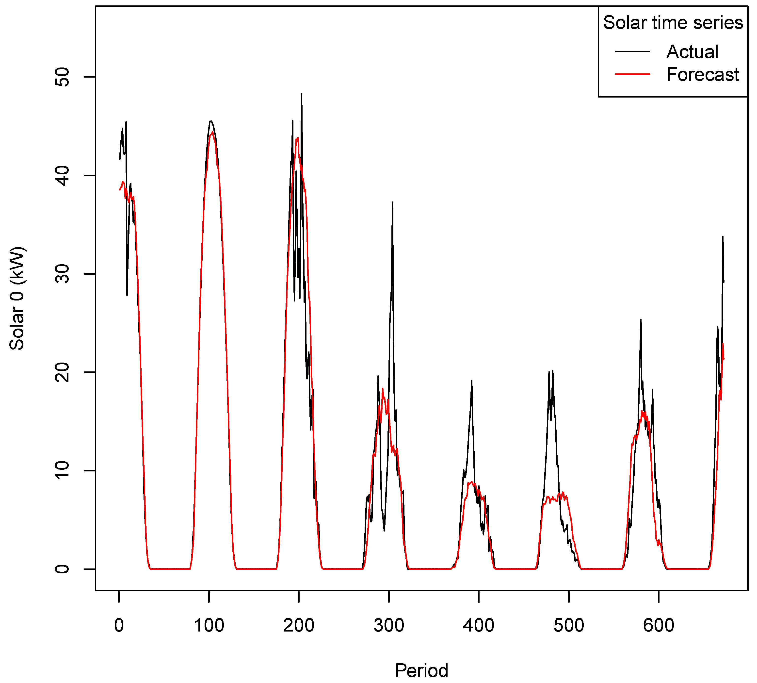
- Added cloud cover variables ± 3 h. The effect may be seen in Figure 4 with the predicted solar (black line) beginning to closely match the actual solar (red line) during the day. (MASE 0.6243, 16 October)
- Selected solar data from beginning of 2020 instead of from day 142 (22 May). (MASE 0.6063, 17 October)
- Selected start month (0–8) for each of four building series from 2020, added all possible weather variables, set Building 5 equal to median training value 19 kW (MASE 0.5685, 18 October)
- Fixed up Solar5 data by filtering out values less than 0.05 kW. (MASE 0.5387, 24 October)
- Fixed up Solar0 data by same filtering as for Solar5. (MASE 0.5207, 31 October)
- Added in separate binary decision variables for each day of the week. (MASE 0.5166, 2 November)
| Algorithm 1: Model development for Phase 1. |
|
Figure 4.
Solar 0 Forecast vs Actual (kW)—Phase 1 (1–7 October 2020).

Figure 5.
Building 1 Forecast vs Actual (kW)—Phase 1 (1–7 October 2020).

We were expecting a similar MASE for Phase 2; however, the “reopening” effects of lockdown appeared to result in a reversion to historic usage patterns in some of the buildings, which diverged from our forecast.
Naturally this “reopening” affected all the results of all competitors. In an actual production environment, instead of having a “month-ahead” forecast, the forecasts would be day-ahead and able to rapidly adjust to reopening effects.
Although we do not know the types of the six buildings used in the competition, we surmise that in November 2020 the air-conditioning use of some of them began to revert to the long-term mean. Thus, our approach of choosing different starting months for each building to minimize MASE vis-a-vis October 2020 led to model outperformance.
Model Description
We summarise the predictor variables used in the building and solar modelling and discuss their relative importance.
A list of the 74 predictor variables used in the model for Buildings 0, 1, 3 and 6 is in Table 3. Example values are given for each variable. Similarly, the 39 predictor variables used in the Solar model are shown in Table 4.
These variables are being used to predict the quarter-hour energy usage for each of the buildings; that is, a different model is used for each quarter-hour offset (:00, :15, :30 and :45 of each hour). In the final model, all the solar and building variables (for Buildings 0, 1, 3 and 6) were normalized using the maximum value found in the training data.
The other weather variables (t2m, d2m, wind, MSLP, R, SSRD, STRD and TCC) are the variables provided by OikoLab via the ERA5 model: 2 m temperature, 2 m dewpoint temperature, wind speed, mean sea level pressure, relative humidity, surface solar radiation downward, and surface thermal radiation downward (as seen in Table 1 and Table 2).
The “wh” variable identifies the building being predicted, analogously to the same variable in [10]. Variable name postfixes refer to leading and lagging variables one, two or three hours from the period. Postfixes of 24, 72 and 48 are used for building training—the temperatures 24, 72 and 48 h ago based on the market demand modelling of [12]. These proved to be significant variables in the building energy forecasting.
The variables labelled Moorabbin, Oakleigh and Olympic are repeated values for the BOM daily solar global exposure variables at three sites, i.e., in each quarter hour, the variable is assigned the daily solar global exposure for that day, as the value is measured from midnight to midnight.
The variables “sin_hr” and “sin_day” refer to the Fourier terms related to the hour of the day and the day of the year (Julian date). Thus, and and similarly for the cosine term. These terms model the diurnal and annual cycle in the building energy usage and solar generation. Including these temporal terms, plus the weekday/weekend Boolean variable for the buildings, gives a good first approximation to the building energy usage and solar generation. Competition winning entries such as [72], from the 2014 Global Energy-Forecasting competition, used these terms in both the solar and wind forecasting tracks.
Other variables are binary variables for weekend (“wd”), Monday/Friday (“wd1”), Tuesday/Wednesday/Thursday (“wd2”) and named variables for each day of the week.
For the random forest parameters, each forest was trained with 2000 trees (increased from the default ranger value of 500). The mtry parameter was set to 43 for the forests training buildings 0, 1, 3 and 6 together; to 14 for the forests for Building 1 only; 19 for the forests for Building 6; and 13 for the forests for the solar installations. In ranger, the default mtry parameter is the (floored) square root of the number of independent variables. The variable count is 74 for buildings and 39 for solar; thus, the default mtry parameters would be 8 and 6, respectively, significantly differing from the competition values.
Out of the individuals/teams who made submissions to the evaluation Phase, our entry had the lowest MASE for Phase 2 of 0.6460.
The outperformance is due to many factors including the fine-tuning described above in Section 4.2. We believe that relative to other competitors the approaches of thresholding each building input data set differently, modelling all solar time series together, and including both daily and hourly weather data in the model led to its strong outperformance.
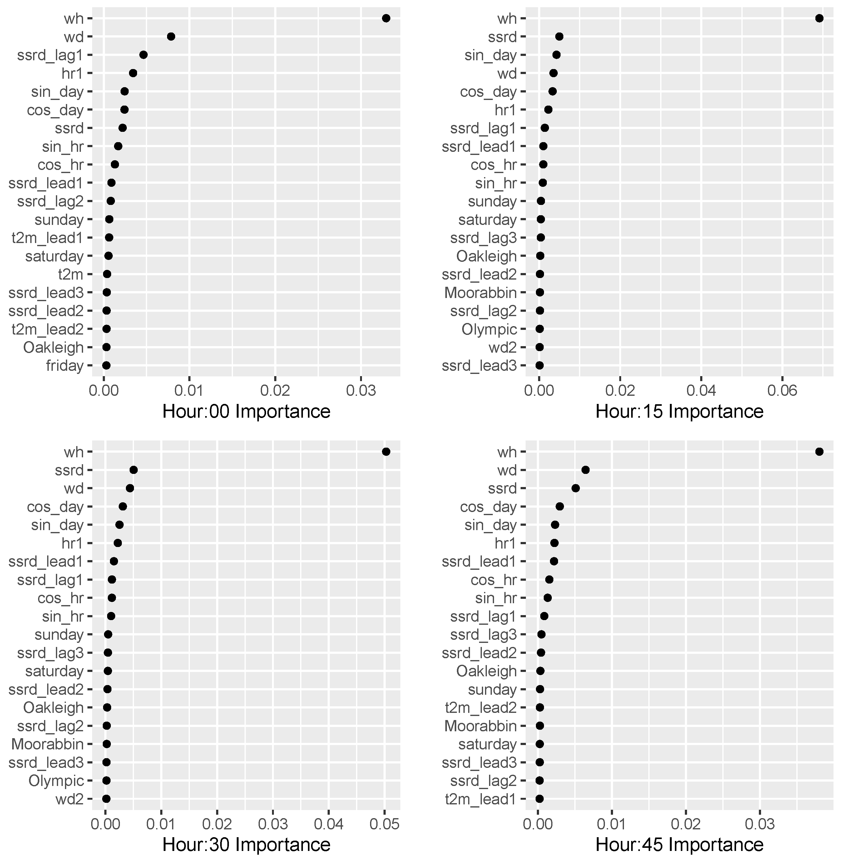
It is difficult to pinpoint the relative contribution of each change, as undoing each change and recalculating the MASE, or even calculating “drop-column importance” for each variable would be very time consuming. Instead, we plot the importance (calculating using permutations in ranger) of the top 20 variables. The plots for the model, for each 15 min offset in an hour, built for Buildings 0, 1, 3 and 6 and the solar model are shown in Figure 6 and Figure 7.
The distance from the Monash campus in a straight line is 3.2 km to Oakleigh, 8.3 km to Moorabbin, and 16.1 km to Olympic Park; this ordering is reflected in the descending order of variable importance in the building and solar models.
For the buildings, the weekday/weekend Boolean variable, followed by the “ssrd” solar variables, the Fourier terms for the hour and Julian date, and the temperature variables are the most important.
For the solar installations, the “ssrd” variables (lagging and leading) followed by the daily BOM solar variables, following by Fourier terms for hour, day and then temperature variables were most important. However, cloud cover, pressure and surface thermal radiation variables (lagging and leading) were still included in the solar model as they improved the performance for Phase 1.
A curious feature of the relative variable importance in the models is seen in the “ssrd” variables; for three of the Building models (:15, :30, and :45), “ssrd” itself is the most important solar variable. But in the four solar models, the important “ssrd” variables are all leading variables and the most important temperature “t2m” variables are also leading variables, often two or three hours into the future.
6. Discussion
After the competition finished, we investigated whether the forecast could have been improved by using extra data that was not mentioned or provided explicitly by the organizers. This could increase the usefulness and generalisability of our model for other applications.
For example, competitors were instructed to download a file of Victorian half-hourly electricity grid pool prices from the Australian Energy Market Operator (AEMO) website for the months of October and November 2020, for use with the optimisation section of the competition. The file also contained electricity demand for the region of Victoria. Changing the URL allowed competitors to access price and demand for all other months.
Elsewhere on the AEMO website, files containing five-minute price and demand (that is, “dispatch period” rather than 30 min “trading period”) data were available. As of 1 July 2021 (after the competition forecast period), the Australian electricity grid has been operated on a “five-minute settlement” basis [73]. This means that generators are paid for their output based on a pool price which changes every five minutes, including in the Victoria region.
Microgrids can be run as direct market participants; that is, it could be envisaged that building air conditioning, for example, could be ramped up or down depending on the real-time pool price. It is not known if the competition microgrid was being operated in this way. The microgrid could be operated based on half-hourly pool prices, although market participants can also see the five-minute pool prices.
The Australian Bureau of Meteorology provides one-minute solar data from the nearby Tullamarine Airport [74] while the City of Melbourne provides 15 min microclimate sensor readings [75].
Other numerical weather prediction (NWP) data are available. As noted above, other published solar models use different variables from the ERA5 data set. The variables at the exact site location were obtained by OikoLab through the process of bilinearly interpolating the nearest four ERA5 data points. Using only the magnitude of the wind rather than its direction removes nuance from the wind data. Inverse distance weighting the four points is another possible technique that could be used to interpolate between the ERA5 data points. The usual exponent used is 2 as in the original paper [76] but this can be varied; see for example [77].
From the ECMWF, higher-resolution data known as ERA5-Land [78] is available, which covers the same variables at a 0.1 × 0.1 degree grid resolution, except for cloud cover. For the competition site, however, only three points on land were available.
The Japanese Meteorological Agency provides JRA-55 historical reanalysis data at a 3-hourly, 0.5625 degree resolution [79] and the NCEP in the US provides GFS (Global Forecasting System reanalysis data) at a 3-hourly, 0.25 degree resolution [80]. The JRA-55 reanalysis point was located only 400 m away from the microgrid.
Finally, the US National Aeronautics and Space Administration (NASA) provides data from MERRA-2 [81] at an hourly, 0.5 latitude × 0.625 longitude degree resolution, examined in [61]; the model “SWGNT” variable can be used for the solar radiation downwards variable.
The website “pvoutput.org” [82] allows users who donate to download historical data from photovoltaic installations. Such data can be available at 5 min resolution. These data are used in the Australian Solar Energy Forecasting System (ASEFS) of AEMO [83] and are available at several sites near the microgrid. Similar data are available on a commercial basis from a different company [84].
The “Weatherman” paper [85] described a method for determining the parameters of a solar installation by examining time series data of its output, and then estimating its size, location, angle of inclination, and orientation. A similar approach was implemented to locate a house using PV data in [86] based on ECMWF data and PV simulation. This approach may also have been useful in this and similar competitions, but could not pursued due to lack of time.
Including AEMO 5-minute Victorian demand reduced the Phase 1 MASE slightly (final average MASE 0.6395) while including AEMO 5-minute price data or MERRA-2 solar data reduced the MASE by similar amounts.
In any case, including AEMO price or demand data (forecasts) in a production model may not be realistic, unless the microgrid trades in the wholesale electricity market. Additionally, MERRA-2 and JRA-55 are purely “reanalysis” data and thus no corresponding forecast is currently available, as for BOM and ECMWF data.
Ultimately, it was determined that only the one-minute BOM solar data and PVOutput.org data provided significant improvements in the competition framework.
Table 5 shows the MASE for six competitors’ entries. The building and solar MASE values are labelled “b” and “s”, respectively. The mean MASE over all 12 time-series values for Phase 2 is shown in the top row. This was the benchmark used for the forecasting prize of the competition.
Our error rates are in the column labelled “1” while those for five other entrants are labelled “2” to “6” for comparison (2, 3 and 4 were ranked second, third and fourth). The last two columns labelled “BOM” and “PVO” show the MASE when one-minute BOM solar data from Tullamarine Airport is included and when the 15-min solar output (from PVOutput.org) of seven houses nearby is added to the model (without adjusting any other model parameters). In the last case, at almost all houses, the 15-min solar data for 2019 and 2020 is missing at least one data point. This limited the number of houses in the vicinity to seven.
For the last “PVO” case, the solar MASEs are all in the range 0.22 to 0.35 (down from 0.38 to 0.60 in the submitted solution). It is noteworthy that the Building 1 MASE also decreases with the addition of these variables.
Adding one-minute solar data from the Tullamarine Airport, which is 37.7 km from the site in great circle distance, has a much smaller effect, with the solar MASEs in the range 0.34 to 0.54.
As including these extra variables lowers the MASE significantly, a practical finding is that competition winners should open-source their code for review not just by competition organizers but the public. This should be communicated from the competition outset. An example from Kaggle showed how hidden code was detected long after prizes were awarded [87]. The possibility of competitors using these extra variables in an intermediate step before the final solution cannot be excluded.
7. Conclusions
To forecast 15-min energy and solar time-series data, we applied the quantile regression forest of [66] based on the original random forest idea of [65] as provided in the R ranger package [70]. This was highly effective in conjunction with techniques of thresholding, grouping related buildings and solar installations, combining daily and hourly data from two uncorrelated data sources, and normalization. The quantile regression forest approach was ideal as it required minimal parameter tuning and thus the process of building and testing models was expedited in the time-pressured environment of the competition. Other more complex approaches such as gradient boosting machines may have required more parameter tuning.
In the training phase, the training data for each building and solar installation was extended backwards from the latest available data, month by month, until the error rate for each building or solar time series began to increase. In a production environment as opposed to a competition, this approach should be verified by performing cross-validation. This approach of grouping and thresholding may have captured different building types present on campus and their differing response to reopening, as seen in studies of the effect of COVID-19 lockdowns on energy at university campuses worldwide.
The success of combining daily solar exposure data from the Australian BOM with hourly weather data from the ECMWF appeared to play a large part in the outperformance of our approach versus the other contest entrants.
For real-world forecasting, it is beneficial to take the performance of private PV systems into account; sites such as PVOutput.org can help in this case.
Further research could include studying the relative effect of each change, the potential effect of interpolating weather variables differently, and testing other machine-learning algorithms. In particular, it would be useful to generalize the approach of grouping related buildings and solar installations. For the generalization from this microgrid to, for example, houses in a larger electricity grid, the time-series grouping [88] could be based on different kinds of houses, residents, and aspects of solar installations, and could be derived automatically rather than manually as in this competition.
Funding
This work was partially supported by funding from Project SHIELD of the Australian Renewable Energy Agency.
Data Availability Statement
Data and code for this study may be found at [89].
Conflicts of Interest
The authors declare no conflict of interest.
References
- Elmachtoub, A.N.; Grigas, P. Smart “predict, then optimize”. Manag. Sci. 2022, 68, 9–26. [Google Scholar] [CrossRef]
- Bergmeir, C.; de Nijs, F.; Sriramulu, A.; Abolghasemi, M.; Bean, R.; Betts, J.; Bui, Q.; Dinh, N.T.; Einecke, N.; Esmaeilbeigi, R.; et al. Comparison and Evaluation of Methods for a Predict+ Optimize Problem in Renewable Energy. arXiv 2022, arXiv:2212.10723. [Google Scholar]
- Hyndman, R.J.; Koehler, A.B. Another look at measures of forecast accuracy. Int. J. Forecast. 2006, 22, 679–688. [Google Scholar] [CrossRef] [Green Version]
- Hong, T.; Pinson, P.; Fan, S.; Zareipour, H.; Troccoli, A.; Hyndman, R.J. Probabilistic energy forecasting: Global energy forecasting competition 2014 and beyond. Int. J. Forecast. 2016, 32, 896–913. [Google Scholar] [CrossRef] [Green Version]
- Hong, T.; Xie, J.; Black, J. Global Energy Forecasting Competition 2017: Hierarchical probabilistic load forecasting. Int. J. Forecast. 2019, 35, 1389–1399. [Google Scholar] [CrossRef]
- Hong, T.; Pinson, P.; Fan, S. Global energy forecasting competition 2012. Int. J. Forecast. 2014, 30, 357–363. [Google Scholar] [CrossRef]
- Charlton, N.; Singleton, C. A refined parametric model for short term load forecasting. Int. J. Forecast. 2014, 30, 364–368. [Google Scholar] [CrossRef] [Green Version]
- Gaillard, P.; Goude, Y.; Nedellec, R. Additive models and robust aggregation for GEFCom2014 probabilistic electric load and electricity price forecasting. Int. J. Forecast. 2016, 32, 1038–1050. [Google Scholar] [CrossRef]
- Nagy, G.I.; Barta, G.; Kazi, S.; Borbély, G.; Simon, G. GEFCom2014: Probabilistic solar and wind power forecasting using a generalized additive tree ensemble approach. Int. J. Forecast. 2016, 32, 1087–1093. [Google Scholar] [CrossRef]
- Smyl, S.; Hua, N.G. Machine learning methods for GEFCom2017 probabilistic load forecasting. Int. J. Forecast. 2019, 35, 1424–1431. [Google Scholar] [CrossRef]
- Aggarwal, S.; Saini, L. Solar energy prediction using linear and non-linear regularization models: A study on AMS (American Meteorological Society) 2013–14 Solar Energy Prediction Contest. Energy 2014, 78, 247–256. [Google Scholar] [CrossRef]
- Clements, A.E.; Hurn, A.; Li, Z. Forecasting day-ahead electricity load using a multiple equation time series approach. Eur. J. Oper. Res. 2016, 251, 522–530. [Google Scholar] [CrossRef] [Green Version]
- Li, Z.; Hurn, A.; Clements, A. Forecasting quantiles of day-ahead electricity load. Energy Econ. 2017, 67, 60–71. [Google Scholar] [CrossRef] [Green Version]
- Abuella, M.; Chowdhury, B. Random forest ensemble of support vector regression models for solar power forecasting. In Proceedings of the 2017 IEEE Power & Energy Society Innovative Smart Grid Technologies Conference (ISGT), Washington, DC, USA, 23–26 April 2017; pp. 1–5. [Google Scholar] [CrossRef] [Green Version]
- Abolghasemi, M.; Esmaeilbeigi, R. State-of-the-art predictive and prescriptive analytics for IEEE CIS 3rd Technical Challenge. arXiv 2021, arXiv:2112.03595. [Google Scholar]
- Bean, R. Methodology for forecasting and optimization in IEEE-CIS 3rd Technical Challenge. arXiv 2022, arXiv:2202.00894. [Google Scholar]
- Limmer, S.; Einecke, N. An Efficient Approach for Peak-Load-Aware Scheduling of Energy-Intensive Tasks in the Context of a Public IEEE Challenge. Energies 2022, 15, 3718. [Google Scholar] [CrossRef]
- Stratigakos, A. A Robust Fix-and-Optimize Matheuristic for Timetabling Problems with Uncertain Renewable Energy Production. Available online: https://hal.archives-ouvertes.fr/hal-03449920/document (accessed on 24 November 2022).
- Yuan, R.; Dinh, N.T.; Pipada, Y.; Pourmouasvi, S.A. Optimal activity and battery scheduling algorithm using load and solar generation forecast. arXiv 2021, arXiv:2112.02827. [Google Scholar]
- Ruddick, J.; Genov, E.; Camargo, L.R.; Coosemans, T.; Messagie, M. Evolutionary scheduling of university activities based on consumption forecasts to minimise electricity costs. arXiv 2022, arXiv:2202.12595. [Google Scholar]
- Zhu, Q.; Xu, Y.; Dong, M.; Cai, J.; Ji, J.; Lin, Q. A Local Search Method for Solving a Bi-Level Timetabling and Battery Scheduling Problem. Available online: https://github.com/xuyaojian123/IEEE-Predict-Optimize-Challenge/blob/master/IEEE_Conference_Template.pdf (accessed on 24 November 2022).
- Abolghasemi, M.; Bean, R. How to predict and optimise with asymmetric error metrics. arXiv 2022, arXiv:2211.13586. [Google Scholar]
- Hewamalage, H.; Ackermann, K.; Bergmeir, C. Forecast Evaluation for Data Scientists: Common Pitfalls and Best Practices. arXiv 2022, arXiv:2203.10716. [Google Scholar] [CrossRef]
- Perkins, H. Congrats to CRW! Available online: https://www.kaggle.com/competitions/global-energy-forecasting-competition-2012-load-forecasting/discussion/3032 (accessed on 24 November 2022).
- Kolassa, S. Evaluating predictive count data distributions in retail sales forecasting. Int. J. Forecast. 2016, 32, 788–803. [Google Scholar] [CrossRef]
- Kolassa, S. Why the “best” point forecast depends on the error or accuracy measure. Int. J. Forecast. 2020, 36, 208–211. [Google Scholar] [CrossRef]
- Makridakis, S.; Spiliotis, E.; Assimakopoulos, V. The M4 Competition: Results, findings, conclusion and way forward. Int. J. Forecast. 2018, 34, 802–808. [Google Scholar] [CrossRef]
- Petropoulos, F.; Apiletti, D.; Assimakopoulos, V.; Babai, M.Z.; Barrow, D.K.; Taieb, S.B.; Bergmeir, C.; Bessa, R.J.; Bijak, J.; Boylan, J.E.; et al. Forecasting: Theory and practice. Int. J. Forecast. 2022, 38, 705–871. [Google Scholar] [CrossRef]
- Nti, I.K.; Teimeh, M.; Nyarko-Boateng, O.; Adekoya, A.F. Electricity load forecasting: A systematic review. J. Electr. Syst. Inf. Technol. 2020, 7, 1–19. [Google Scholar] [CrossRef]
- Kuster, C.; Rezgui, Y.; Mourshed, M. Electrical load forecasting models: A critical systematic review. Sustain. Cities Soc. 2017, 35, 257–270. [Google Scholar] [CrossRef]
- Zor, K.; Timur, O.; Teke, A. A state-of-the-art review of artificial intelligence techniques for short-term electric load forecasting. In Proceedings of the 2017 6th International Youth Conference on Energy (IYCE), Budapest, Hungary, 21–24 June 2017; pp. 1–7. [Google Scholar] [CrossRef]
- Aguilar Madrid, E.; Antonio, N. Short-term electricity load forecasting with machine learning. Information 2021, 12, 50. [Google Scholar] [CrossRef]
- He, W. Load forecasting via deep neural networks. Procedia Comput. Sci. 2017, 122, 308–314. [Google Scholar] [CrossRef]
- Bessec, M.; Fouquau, J. Short-run electricity load forecasting with combinations of stationary wavelet transforms. Eur. J. Oper. Res. 2018, 264, 149–164. [Google Scholar] [CrossRef]
- Wen, L.; Zhou, K.; Yang, S. Load demand forecasting of residential buildings using a deep learning model. Electr. Power Syst. Res. 2020, 179, 106073. [Google Scholar] [CrossRef]
- Sharifzadeh, M.; Sikinioti-Lock, A.; Shah, N. Machine-learning methods for integrated renewable power generation: A comparative study of artificial neural networks, support vector regression, and Gaussian Process Regression. Renew. Sustain. Energy Rev. 2019, 108, 513–538. [Google Scholar] [CrossRef]
- Zhang, J.; Wei, Y.M.; Li, D.; Tan, Z.; Zhou, J. Short term electricity load forecasting using a hybrid model. Energy 2018, 158, 774–781. [Google Scholar] [CrossRef]
- López, C.; Zhong, W.; Zheng, M. Short-term electric load forecasting based on wavelet neural network, particle swarm optimization and ensemble empirical mode decomposition. Energy Procedia 2017, 105, 3677–3682. [Google Scholar] [CrossRef]
- Voyant, C.; Notton, G.; Kalogirou, S.; Nivet, M.L.; Paoli, C.; Motte, F.; Fouilloy, A. Machine learning methods for solar radiation forecasting: A review. Renew. Energy 2017, 105, 569–582. [Google Scholar] [CrossRef]
- Snow, S.; Bean, R.; Glencross, M.; Horrocks, N. Drivers behind residential electricity demand fluctuations due to COVID-19 restrictions. Energies 2020, 13, 5738. [Google Scholar] [CrossRef]
- Gui, X.; Gou, Z.; Zhang, F.; Yu, R. The impact of COVID-19 on higher education building energy use and implications for future education building energy studies. Energy Build. 2021, 251, 111346. [Google Scholar] [CrossRef] [PubMed]
- Khoshbakht, M.; Gou, Z.; Dupre, K. Energy use characteristics and benchmarking for higher education buildings. Energy Build. 2018, 164, 61–76. [Google Scholar] [CrossRef] [Green Version]
- Chihib, M.; Salmerón-Manzano, E.; Chourak, M.; Perea-Moreno, A.J.; Manzano-Agugliaro, F. Impact of the COVID-19 Pandemic on the Energy Use at the University of Almeria (Spain). Sustainability 2021, 13, 5843. [Google Scholar] [CrossRef]
- Gaspar, K.; Gangolells, M.; Casals, M.; Pujadas, P.; Forcada, N.; Macarulla, M.; Tejedor, B. Assessing the impact of the COVID-19 lockdown on the energy consumption of university buildings. Energy Build. 2022, 257, 111783. [Google Scholar] [CrossRef]
- Nasir, S.N.S.; Ludin, N.A.; Radzi, A.A.S.M.; Junedi, M.M.; Ramli, N.; Marsan, A.; Mohd, Z.F.A.; Roslan, M.R.; Taip, Z.A. Lockdown impact on energy consumption in university building. Environ. Dev. Sustain. 2022, 1–20. [Google Scholar] [CrossRef]
- Huang, Z.; Gou, Z. Electricity consumption variation of public buildings in response to COVID-19 restriction and easing policies: A case study in Scotland, UK. Energy Build. 2022, 267, 112149. [Google Scholar] [CrossRef] [PubMed]
- Farrokhabadi, M.; Browell, J.; Wang, Y.; Makonin, S.; Su, W.; Zareipour, H. Day-Ahead Electricity Demand Forecasting Competition: Post-COVID Paradigm. IEEE Open Access J. Power Energy 2022, 9, 185–191. [Google Scholar] [CrossRef]
- Makridakis, S.; Spiliotis, E.; Assimakopoulos, V. The M5 competition: Background, organization, and implementation. Int. J. Forecast. 2022, 38, 1325–1336. [Google Scholar] [CrossRef]
- De Vilmarest, J.; Goude, Y. State-Space Models Win the IEEE DataPort Competition on Post-covid Day-ahead Electricity Load Forecasting. arXiv 2021, arXiv:2110.00334. [Google Scholar]
- Obst, D.; De Vilmarest, J.; Goude, Y. Adaptive methods for short-term electricity load forecasting during COVID-19 lockdown in France. IEEE Trans. Power Syst. 2021, 36, 4754–4763. [Google Scholar] [CrossRef]
- Ziel, F. Smoothed Bernstein Online Aggregation for Short-Term Load Forecasting in IEEE DataPort Competition on Day-Ahead Electricity Demand Forecasting: Post-COVID Paradigm. IEEE Open Access J. Power Energy 2022, 9, 202–212. [Google Scholar] [CrossRef]
- Bureau of Meteorology. Climate Data Online. Available online: http://www.bom.gov.au/climate/data/index.shtml (accessed on 24 November 2022).
- Hersbach, H.; Bell, B.; Berrisford, P.; Biavati, G.; Horányi, A.; Muñoz Sabater, J.; Nicolas, J.; Peubey, C.; Radu, R.; Rozum, I.; et al. ERA5 hourly data on single levels from 1979 to present. In Copernicus Climate Change Service (C3S) Climate Data Store (CDS); European Centre for Medium-Range Weather Forecasts: Reading, UK, 2018. [Google Scholar] [CrossRef]
- Hersbach, H.; Bell, B.; Berrisford, P.; Biavati, G.; Horányi, A.; Muñoz Sabater, J.; Nicolas, J.; Peubey, C.; Radu, R.; Rozum, I.; et al. ERA5 hourly data on pressure levels from 1979 to present. In Copernicus Climate Change Service (C3S) Climate Data Store (CDS); European Centre for Medium-Range Weather Forecasts: Reading, UK, 2018. [Google Scholar] [CrossRef]
- Yang, J. OikoLab. Available online: https://www.oikolab.com (accessed on 24 November 2022).
- Espejo, F.A.; Grillo, S.; Luini, L. Photovoltaic Power Production Estimation Based on Numerical Weather Predictions. In Proceedings of the 2019 IEEE Milan PowerTech, Milan, Italy, 23–27 June 2019; pp. 1–6. [Google Scholar] [CrossRef]
- Yang, D.; Wang, W.; Hong, T. A historical weather forecast dataset from the European Centre for Medium-Range Weather Forecasts (ECMWF) for energy forecasting. Sol. Energy 2022, 232, 263–274. [Google Scholar] [CrossRef]
- Open Energy Modelling Framework. Feedinlib. Available online: https://github.com/oemof/feedinlib/blob/dev/src/feedinlib/era5.py (accessed on 24 November 2022).
- GRECO Project. PVCompare. Available online: https://github.com/greco-project/pvcompare/blob/dev/pvcompare/era5.py (accessed on 24 November 2022).
- European Centre for Medium-Range Weather Forecasts. GRIB Parameter Database. Available online: https://apps.ecmwf.int/codes/grib/param-db (accessed on 24 November 2022).
- Camargo, L.R.; Schmidt, J. Simulation of multi-annual time series of solar photovoltaic power: Is the ERA5-Land reanalysis the next big step? Sustain. Energy Technol. Assess. 2020, 42, 100829. [Google Scholar] [CrossRef]
- National Renewable Energy Laboratory. PVLIB. Available online: https://github.com/pvlib/pvlib-python/blob/master/pvlib/iotools/pvgis.py (accessed on 24 November 2022).
- European Commission. Photovoltaic Geographical Information System. Available online: https://ec.europa.eu/jrc/en/pvgis (accessed on 24 November 2022).
- Clean Energy Council. Consumer Guide to Buying Household Solar Panels. Available online: https://www.solarchoice.net.au/wp-content/uploads/Solar-Choice-Clean-Energy-Council-Solar-PV-Consumer-guide.pdf (accessed on 24 November 2022).
- Breiman, L. Random Forests. Mach. Learn. 2001, 45, 5–32. [Google Scholar] [CrossRef] [Green Version]
- Meinshausen, N.; Ridgeway, G. Quantile Regression Forests. J. Mach. Learn. Res. 2006, 7. [Google Scholar] [CrossRef]
- Pierrot, A.; Goude, Y. Short-term electricity load forecasting with generalized additive models. Proc. ISAP Power 2011, 2011, 593–600. [Google Scholar]
- Bean, R.; Pojani, D.; Corcoran, J. How does weather affect bikeshare use? A comparative analysis of forty cities across climate zones. J. Transp. Geogr. 2021, 95, 103155. [Google Scholar] [CrossRef]
- Bean, R.; Khan, H. Using solar and load predictions in battery scheduling at the residential level. arXiv 2018, arXiv:1810.11178. [Google Scholar]
- Wright, M.N.; Ziegler, A. ranger: A fast implementation of random forests for high dimensional data in C++ and R. arXiv 2015, arXiv:1508.04409. [Google Scholar] [CrossRef]
- Wang, P.; Liu, B.; Hong, T. Electric load forecasting with recency effect: A big data approach. Int. J. Forecast. 2016, 32, 585–597. [Google Scholar] [CrossRef] [Green Version]
- Juban, R.; Ohlsson, H.; Maasoumy, M.; Poirier, L.; Kolter, J.Z. A multiple quantile regression approach to the wind, solar, and price tracks of GEFCom2014. Int. J. Forecast. 2016, 32, 1094–1102. [Google Scholar] [CrossRef]
- Australian Energy Market Commission. Five Minute Settlement. Available online: https://www.aemc.gov.au/rule-changes/five-minute-settlement (accessed on 24 November 2022).
- Bureau of Meterology. One Minute Solar Data. Available online: http://www.bom.gov.au/climate/data/oneminsolar/stations.shtml (accessed on 14 December 2022).
- City of Melbourne. Microclimate Sensor Readings. Available online: https://data.melbourne.vic.gov.au/Environment/Microclimate-Sensor-Readings/u4vh-84j8 (accessed on 14 December 2022).
- Shepard, D. A two-dimensional interpolation function for irregularly-spaced data. In Proceedings of the 1968 23rd ACM National Conference, New York, NY, USA, 27–29 August 1968; pp. 517–524. [Google Scholar] [CrossRef]
- Li, Z.; Zhang, X.; Zhu, R.; Zhang, Z.; Weng, Z. Integrating data-to-data correlation into inverse distance weighting. Comput. Geosci. 2020, 24, 203–216. [Google Scholar] [CrossRef]
- Muñoz-Sabater, J.; Dutra, E.; Agustí-Panareda, A.; Albergel, C.; Arduini, G.; Balsamo, G.; Boussetta, S.; Choulga, M.; Harrigan, S.; Hersbach, H.; et al. ERA5-Land: A state-of-the-art global reanalysis dataset for land applications. Earth Syst. Sci. Data 2021, 13, 4349–4383. [Google Scholar] [CrossRef]
- Japan Meteorological Agency. JRA-55: Japanese 55-Year Reanalysis, Daily 3-Hourly and 6-Hourly Data; Research Data Archive at the National Center for Atmospheric Research, Computational and Information Systems Laboratory: Boulder, CO, USA, 2013. [Google Scholar] [CrossRef]
- National Centers for Environmental Prediction; National Weather Service; NOAA; U.S. Department of Commerce. NCEP GFS 0.25 Degree Global Forecast Grids Historical Archive; Research Data Archive at the National Center for Atmospheric Research, Computational and Information Systems Laboratory: Boulder, CO, USA, 2015. [Google Scholar] [CrossRef]
- Global Modelling and Assimilation Office. MERRA-2 tavg1_2d_rad_nx: 2d, 1-Hourly, Time-Averaged, Single-Level, Assimilation, Radiation Diagnostics v5. 12.4; Goddard Earth Sciences Data and Information Services Center (GES DISC): Greenbelt, MD, USA, 2015. [CrossRef]
- PV Output. Available online: https://pvoutput.org (accessed on 24 November 2022).
- Australian Energy Market Operator. Australian Energy Solar Forecasting System. Available online: https://aemo.com.au/en/energy-systems/electricity/national-electricity-market-nem/nem-forecasting-and-planning/operational-forecasting/solar-and-wind-energy-forecasting/australian-solar-energy-forecasting-system (accessed on 24 November 2022).
- Solar Analytics. Available online: https://www.solaranalytics.com.au/ (accessed on 24 November 2022).
- Chen, D.; Irwin, D. Weatherman: Exposing weather-based privacy threats in big energy data. In Proceedings of the 2017 IEEE International Conference on Big Data (Big Data), Boston, MA, USA, 11–14 December 2017; pp. 1079–1086. [Google Scholar] [CrossRef]
- Bean, R.; Zhang, Y.; Ko, R.K.; Mao, X.; Bai, G. Preserving the Privacy and Cybersecurity of Home Energy Data. In Emerging Trends in Cybersecurity Applications; Springer: Berlin, Germany, 2023; pp. 301–322. [Google Scholar] [CrossRef]
- Quach, K. How a Kaggle Grandmaster Cheated in $25,000 AI Contest with Hidden Code—And Was Fired from Dream SV Job. Available online: https://www.theregister.com/2020/01/21/ai_kaggle_contest_cheat/ (accessed on 24 November 2022).
- Hyndman, R.J.; Lee, A.J.; Wang, E. Fast computation of reconciled forecasts for hierarchical and grouped time series. Comput. Stat. Data Anal. 2016, 97, 16–32. [Google Scholar] [CrossRef]
- Bean, R. IEEE Predict Optimize Challenge. Available online: https://github.com/RichardBean/IEEE-Predict-Optimize-Challenge (accessed on 24 November 2022).
Figure 1.
Q-Q plot of all available solar time-series data.

Figure 2.
Building time-series data in kW for October 2020.

Figure 3.
Solar time-series data in kW for October 2020.

Figure 6.
Permutation importance of top 20 variables, Building model.

Figure 7.
Permutation importance of top 20 variables, Solar model.


Table 1.
Description of ECMWF ERA5 variables used in solar models.
| Short Name | Description | Units |
|---|---|---|
| TCLW | Total column cloud liquid water | kg m |
| TCIW | Total column cloud ice water | kg m |
| SP | Surface pressure | Pa |
| TCWV | Total column vertically integrated water vapour | kg m |
| MSL | Mean sea level pressure | Pa |
| R | Relative humidity | % |
| TCC | Total cloud cover | (0–1) |
| 10U | 10 m U wind component | m s |
| 10V | 10 m V wind component | m s |
| 2T | 2 m temperature | K |
| 2D | 2 m dewpoint temperature | K |
| SSRD | Surface solar radiation downwards | J m |
| STRD | Surface thermal radiation downwards | J m |
| TSR | Top net solar radiation | J m |
| LCC | Low cloud cover | (0–1) |
| TCO3 | Total column ozone | kg m |
| TISR | TOA incident solar radiation | J m |
| TP | Total precipitation | m |
| FAL | Forecast albedo | (0–1) |
| FDIR | Total sky direct solar radiation at surface | J m |
| CDIR | Clear-sky direct solar radiation at surface | J m |
| SSRDC | Surface solar radiation downward clear-sky | J m |
Table 2.
Comparison of ECMWF ERA5 variables used in solar models.
| ID | Name | GEFCOM 2014 [4] | IEEE-CIS [2] | Espejo et al. [56] | Yang et al. [57] | PVLIB [58] | PVCompare [59] |
|---|---|---|---|---|---|---|---|
| 78 | TCLW | 🗸 | |||||
| 79 | TCIW | 🗸 | |||||
| 134 | SP | 🗸 | 🗸 | ||||
| 137 | TCWV | 🗸 | 🗸 | ||||
| 151 | MSL | 🗸 | |||||
| 157 | R | 🗸 | 🗸 | ||||
| 164 | TCC | 🗸 | 🗸 | ||||
| 165 | 10U | 🗸 | 🗸 | 🗸 | 🗸 | 🗸 | |
| 166 | 10V | 🗸 | 🗸 | 🗸 | 🗸 | ||
| 167 | 2T | 🗸 | 🗸 | 🗸 | 🗸 | 🗸 | 🗸 |
| 168 | 2D | 🗸 | 🗸 | ||||
| 169 | SSRD | 🗸 | 🗸 | 🗸 | 🗸 | 🗸 | 🗸 |
| 175 | STRD | 🗸 | 🗸 | 🗸 | |||
| 178 | TSR | 🗸 | |||||
| 186 | LCC | 🗸 | |||||
| 206 | TCO3 | 🗸 | |||||
| 212 | TISR | 🗸 | |||||
| 228 | TP | 🗸 | 🗸 | ||||
| 243 | FAL | 🗸 | |||||
| 228021 | FDIR | 🗸 | 🗸 | 🗸 | 🗸 | ||
| 228022 | CDIR | 🗸 | |||||
| 228129 | SSRDC | 🗸 | |||||
| # | 12 | 8 | 5 | 14 | 5 | 6 |
Table 3.
Building predictor variables.
| wh | 6 | t2m_lead1 | 10.2 | strd_lead1 | 319 | rh_lag1 | 0.87 | sin_hr | 0 |
| t2m | 9.7 | t2m_lead2 | 10.7 | strd_lead2 | 328 | rh_lag2 | 0.87 | cos_hr | 1 |
| d2m | 7.3 | t2m_lead3 | 10.6 | strd_lead3 | 334 | rh_lag3 | 0.86 | wd | 0 |
| wind | 5 | t2m_lag24 | 13.8 | wind_lag1 | 4.6 | rh_lead1 | 0.82 | wd1 | 1 |
| mslp | 1005 | t2m_lag24 | 13.4 | wind_lag2 | 4.4 | rh_lead2 | 0.8 | wd2 | 0 |
| rh | 0.85 | t2m_lag72 | 12.3 | wind_lag3 | 6.3 | rh_lead3 | 0.83 | sunday | 0 |
| ssrd | 59.4 | ssrd_lag1 | 15.4 | wind_lead1 | 5.7 | cloud_lag1 | 1 | monday | 1 |
| strd | 338.4 | ssrd_lag2 | 1.1 | wind_lead2 | 5.9 | cloud_lag2 | 1 | tuesday | 0 |
| cloud | 1 | ssrd_lag3 | 0 | wind_lead3 | 5.8 | cloud_lag3 | 1 | wednesday | 0 |
| Moorabbin | 4.5 | ssrd_lead1 | 182 | d2m_lag1 | 7.6 | cloud_lead1 | 0.97 | thursday | 0 |
| Oakleigh | 2.8 | ssrd_lead2 | 244 | d2m_lag2 | 7.7 | cloud_lead2 | 0.99 | friday | 0 |
| Olympic | 2.6 | ssrd_lead3 | 152 | d2m_lag3 | 7.9 | cloud_lead3 | 0.99 | saturday | 0 |
| t2m_lag1 | 9.7 | strd_lag1 | 344 | d2m_lead1 | 7.3 | mslp_lag1 | 1005 | sin_day | 0.5 |
| t2m_lag2 | 9.8 | strd_lag2 | 347 | d2m_lead2 | 7.3 | mslp_lead1 | 1005 | cos_day | −0.87 |
| t2m_lag3 | 10.1 | strd_lag3 | 345 | d2m_lead3 | 7.8 | hr1 | 0 | x1 | 0.63 |
Table 4.
Solar predictor variables.
| wh | 0 | t2m_lag2 | 12 | ssrd_lead3 | 0.66 | cloud_lead1 | 0.48 |
| t2m | 12 | t2m_lag3 | 12 | strd_lag1 | 318 | cloud_lead2 | 0.58 |
| mslp | 1018 | t2m_lead1 | 12 | strd_lag2 | 332 | cloud_lead3 | 0.74 |
| ssrd | 203 | t2m_lead2 | 11 | strd_lag3 | 347 | mslp_lag1 | 1017 |
| strd | 321 | t2m_lead3 | 10 | strd_lead1 | 311 | mslp_lead1 | 1018 |
| cloud | 0.37 | ssrd_lag1 | 221 | strd_lead2 | 308 | sin_hr | 0.97 |
| Moorabbin | 8.8 | ssrd_lag2 | 172 | strd_lead3 | 303 | cos_hr | 0.26 |
| Oakleigh | 8 | ssrd_lag3 | 173 | cloud_lag1 | 0.56 | sin_day | 0.66 |
| Olympic | 6.6 | ssrd_lead1 | 145 | cloud_lag2 | 0.81 | cos_day | −0.76 |
| t2m_lag1 | 12 | ssrd_lead2 | 54 | cloud_lag3 | 0.94 | x1 | 0 |
Table 5.
Comparison of MASE for entries and with improvements.
| 1 | 2 | 3 | 4 | 5 | 6 | BOM | PVO | |
|---|---|---|---|---|---|---|---|---|
| Mean | 0.6460 | 0.7441 | 0.7750 | 0.8073 | 0.8474 | 1.0026 | 0.6217 | 0.5434 |
| b0 | 1.0438 | 0.9081 | 0.9413 | 1.2008 | 1.3227 | 1.2376 | 1.0407 | 1.0383 |
| b1 | 0.8840 | 0.9610 | 1.0171 | 1.1341 | 1.0362 | 1.1077 | 0.8881 | 0.8594 |
| b3 | 0.6494 | 0.7524 | 0.6099 | 0.6398 | 0.7785 | 0.7711 | 0.6501 | 0.6610 |
| b4 | 0.7236 | 0.6775 | 0.7236 | 0.8096 | 0.8269 | 0.7236 | 0.7236 | 0.7236 |
| b5 | 0.7922 | 0.9654 | 0.8563 | 0.9493 | 0.8463 | 0.9157 | 0.7922 | 0.7922 |
| b6 | 0.7476 | 0.7822 | 0.8611 | 1.0182 | 0.8577 | 0.7694 | 0.7460 | 0.7494 |
| s0 | 0.6019 | 0.9305 | 0.9159 | 1.0439 | 1.0170 | 1.4421 | 0.5425 | 0.3513 |
| s1 | 0.3860 | 0.4187 | 0.5222 | 0.3988 | 0.5416 | 0.8155 | 0.3468 | 0.2399 |
| s2 | 0.4148 | 0.5314 | 0.6186 | 0.5248 | 0.6656 | 0.9462 | 0.3727 | 0.2234 |
| s3 | 0.5475 | 0.7032 | 0.6678 | 0.7221 | 0.7118 | 1.0440 | 0.5048 | 0.3470 |
| s4 | 0.4179 | 0.5616 | 0.6516 | 0.5173 | 0.7002 | 0.9947 | 0.3727 | 0.2620 |
| s5 | 0.5435 | 0.7366 | 0.9145 | 0.7289 | 0.8639 | 1.2640 | 0.4799 | 0.2734 |
Disclaimer/Publisher’s Note: The statements, opinions and data contained in all publications are solely those of the individual author(s) and contributor(s) and not of MDPI and/or the editor(s). MDPI and/or the editor(s) disclaim responsibility for any injury to people or property resulting from any ideas, methods, instructions or products referred to in the content. |
© 2023 by the author. Licensee MDPI, Basel, Switzerland. This article is an open access article distributed under the terms and conditions of the Creative Commons Attribution (CC BY) license (https://creativecommons.org/licenses/by/4.0/).
Share and Cite
MDPI and ACS Style
Bean, R. Forecasting the Monash Microgrid for the IEEE-CIS Technical Challenge. Energies 2023, 16, 1050. https://doi.org/10.3390/en16031050
AMA Style
Bean R. Forecasting the Monash Microgrid for the IEEE-CIS Technical Challenge. Energies. 2023; 16(3):1050. https://doi.org/10.3390/en16031050
Chicago/Turabian StyleBean, Richard. 2023. "Forecasting the Monash Microgrid for the IEEE-CIS Technical Challenge" Energies 16, no. 3: 1050. https://doi.org/10.3390/en16031050
Note that from the first issue of 2016, this journal uses article numbers instead of page numbers. See further details here.