Article

Price-Based Demand Response: A Three-Stage Monthly Time-of-Use Tariff Optimization Model

1
State Grid Energy Research Institute Co., Ltd., Beijing 102209, China
2
Marketing Service Center of State Grid Chongqing Electric Power Company, Chongqing 400023, China
3
School of Economics and Management, North China Electric Power University, Beijing 102206, China
*
Author to whom correspondence should be addressed.
Energies 2023, 16(23), 7858; https://doi.org/10.3390/en16237858
Submission received: 30 October 2023 / Revised: 22 November 2023 / Accepted: 25 November 2023 / Published: 30 November 2023
(This article belongs to the Special Issue Demand Response Optimization Techniques for Smart Power Grids 2023)

Abstract

:
In this research, we developed a three-stage monthly time-of-use (TOU) tariff optimization model to address the concerns of confusing time period division, illogical price setting, and incomplete seasonal element consideration in the previous TOU tariff design. The empirical investigation was conducted based on load, power generation, and electricity pricing data from a typical northwest region in China in 2022. The findings indicate the following: (1) In producing the typical net load curves, the employed K-means++ technique outperformed the standard models in terms of the clustering effect by 4.27–26.70%. (2) Following optimization, there was a decrease of 1900 MW in the maximum monthly abandonment of renewable energy, a decrease of 0.31–53.94% in the peak–valley difference, and a decrease of 2.03–17.27% in the monthly net load cost. (3) By taking extra critical peak and deep valley time periods into account, the average net load cost decreased by 10.36% compared with conventional peak–flat–valley time period division criteria.

1. Introduction

1.1. Background and Motivation

To address the increasingly severe issue of climate change, countries around the globe are committed to reducing greenhouse gas emissions and proposing proactive and feasible net-zero emission goals [1]. Considering the low-carbon and environmentally friendly characteristics of renewable energy, constructing a power system dominated by high-penetration renewable energy sources is an important measure for the power industry to achieve net-zero emission goals [2]. However, renewable energy generation has the characteristics of randomness and volatility, which affect the safe and stable operation of power systems, thus bringing new challenges to the power industry [3]. Therefore, it is of great significance to vigorously promote the development of flexible resources (FRs) [4]. 
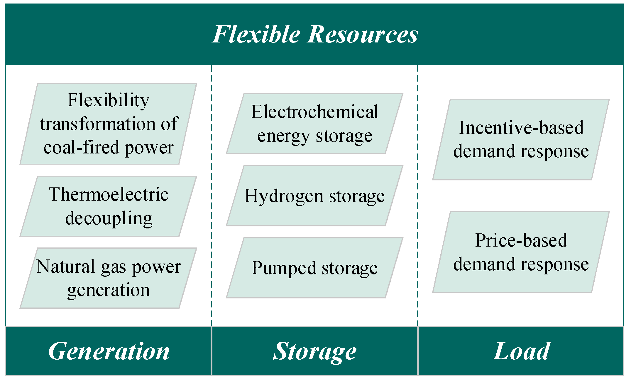
Figure 1 depicts the main components of FRs in a power system.
However, this requires significant financial outlays, as well as time, either on the generation side (transforming conventional power sources) or the storage side (building energy storage systems). In contrast, it is definitely more economical and sustainable to carry out demand response (DR) on the load side [5]. According to the response method, DR can be further divided into incentive-based demand response (IDR) and price-based demand response (PDR). Of these, the former emphasizes that users adjust their electricity demand at appropriate times to obtain corresponding subsidies, and the latter reflects that users are guided by price signals and spontaneously adjust their electricity consumption [6,7]. Figure 2 depicts the main components of IDR and PDR.
As one of the PDRs, the time-of-use (TOU) tariff is formulated by the government and is more feasible and manageable compared with the real-time electricity prices (RTPs) determined by the market [8]. Hence, TOU is still the main electricity pricing method implemented in most regions, especially in areas where the construction of the electricity market is in the early stages. The basic principle of the TOU tariff is to guide users to optimize their electricity consumption behavior and achieve “peak-cutting” and “valley-filling” by dividing the 24 h day into several time periods and assigning different tariff levels to different time periods [9,10]. However, there are three main issues in formulating a scientifically reasonable TOU tariff:
  • How could we divide different time periods?
  • How could we set different tariffs for each time period?
  • How could we set different tariffs for each season/month?
The answers to the aforementioned queries may aid in the more effective release of price signals that direct consumers to spontaneously modify their electricity use habits. On the one hand, power consumers have the option to select alternative ways to consume electricity during different time periods, which is more cost-effective than paying the same tariff all the time. On the other hand, by raising the rates during times of peak electricity consumption, the power grid can lessen the electrical congestion. As we progressively approach carbon neutrality, in the future, renewable energy will become increasingly prevalent. Simultaneously, the penetration rate of renewable energy will further increase. Expanding the FRs, like flexible power sources and energy storage systems, is not a feasible solution. In comparison, encouraging power customers to cut back on their unnecessary consumption through the guidance of the TOU tariff is more practically significant.

1.2. Implementation Status of the TOU Tariff

Globally, the TOU tariff is widely implemented. However, due to differences in users’ composition and load characteristics, the TOU settings vary greatly in different regions. Taking California (US) and New South Wales (Australia) as examples, the time period division and seasonal setting are shown in Table 1.
As the world’s largest power entity, China’s electricity generation totaled 8534.3 terawatt-hours in 2021, accounting for 29.98% of the global total electricity generated (BP: https://www.bp.com/ (accessed on 16 November 2023)). In an effort to conserve electricity resources and encourage reasonable electricity consumption, China’s central and southwestern areas started experimenting with the TOU tariff in 1984. With the steady improvement of the pricing mechanism, the TOU tariff has expanded and been applied in the majority of China’s regions. However, due to China’s power industry being new, the TOU tariff implemented in most regions still needs to be improved. In 2021, the National Development and Reform Commission (NDRC) announced the following goals for the optimization of the TOU tariff:
  • To improve the TOU tariff pricing mechanism via scientific time period division and establishing a reasonable tariff difference.
  • To establish a critical peak tariff mechanism.
  • To establish a sound seasonal electricity pricing mechanism.
As of November 2022, the implementation of the TOU tariff in 31 regions in China (excluding Tibet, Hong Kong, Macau, and Taiwan) is shown in Table 2.
As shown in Table 2, in various regions of China, there are the following issues:
  • Unreasonable peak–valley tariff ratio
As the regulation states, each region’s peak–valley tariff ratio should not be less than 3:1 in principle. In areas where there are notable peak–valley load differences, the peak–valley tariff ratio might potentially surpass 4:1. Currently, only half of the areas have a peak–valley pricing ratio greater than 3:1, and the majority of the regions continue to comply with the national requirements, without exploring more scientific and practical peak–valley tariff ratios with regional features.
2.
Widely implemented critical peak and unpopular deep valley tariffs
Most regions have established critical peak time periods and tariffs in order to strengthen the TOU tariff. Nonetheless, as renewable energy installations continue to rise, in some areas, the supply of electricity outpaces the demand. Therefore, investigating the creation of a deep valley tariff is important from a practical standpoint. At present, only Shandong and Jiangsu have implemented deep valley tariff policies.
3.
Seasonal tariff with lack of narrow time scales
The majority of regions, aside from Gansu, have implemented thorough seasonal TOU tariff mechanisms. Nevertheless, these tariffs are applied more often in the summer and winter, with little regard for the other seasons. Furthermore, variations persist in the characteristics of loads and the behavior of power consumption even within the same season. For instance, there is a noticeable change in the load for northern cities before and after heating on a day in winter. Hence, it is necessary to set a more refined TOU tariff, such as a monthly tariff.

1.3. Literature Review

The optimization of the TOU tariff is considered a key step in the green and low-carbon energy transformation. To address the aforementioned issues and form a rational TOU tariff, other scholars have also conducted various studies on the optimization of the TOU tariff, as follows:
  • Time period division
The determination of a typical daily load curve is the first step in dividing the time periods. In general, clustering algorithms represented by K-means are the main methods used for determining the typical daily load curves [11]. Considering the strict classification criterion of the K-means algorithm, some scholars also use the fuzzy C-means (FCM) clustering algorithm based on the membership degree to determine the typical daily load curve [12]. However, the position determination of the initial cluster center is the main cause of the final clustering effect, and the above improvement has not solved this problem yet [13]. From the perspective of time period division, in most regions, 24 h is simply divided into three time periods (peak–flat–valley) in a 1:1:1 ratio [14]. Moreover, some existing studies have also followed the same approach to dividing time periods [15].
2.
Price optimization
Power users spontaneously change their power consumption behavior based on the adjustment of electricity prices, thereby achieving the transfer or reduction in power loads. In general, consumers’ psychology analysis and PEED are the two most commonly used methods [16,17]. The former requires simulating the psychological state of the consumers, subjectively setting some parameters. The latter is mainly based on changes in users’ electricity demand and electricity prices, which is more objective [18]. In terms of setting the objective function for price optimization, most existing studies have mainly focused on minimizing the peak–valley difference or maximizing the reduction in peak electricity load [19]. However, with the proposal of carbon neutrality goals, the installed scale of renewable energy continues to expand, resulting in severe wind and light abandonment in some regions [20]. Therefore, it is necessary to consider the absorption of renewable energy when optimizing the TOU tariff.
3.
Execution cycle setting
The setting of the execution cycle is crucial in optimizing the TOU tariff. As with the electricity pricing policies previously implemented in most regions, the execution cycle was set to 1 year in the existing studies [21,22]. In other words, one set of electricity prices is implemented throughout the year. However, due to the seasonal characteristics of climate and electricity consumption behaviors, there are significant differences in the power load among the different months/seasons [23]. Hence, it is more reasonable to carry out differentiated TOU tariff optimization designed around different months/seasons. The existing studies on seasonal TOU tariff optimization mostly concentrate on the summer and winter [24,25], and only a few studies set different prices for the four seasons [26].
Based on the existing literature, several issues exist, as follows:
  • The influence of initial clustering center selection bias is harder to mitigate using most applied clustering models of the typical daily load curve, which leads to inaccuracy in the subsequent procedures. Furthermore, the above research only looked at the load curve on the demand side, and insufficient consideration was given to renewable energy generation on the supply side. This is not sufficiently applicable in light of the increasing penetration of renewable energy.
  • The current literature does not give enough thought to more refined/high-frequency TOU tariff sets (such as monthly TOU tariffs), which may become increasingly crucial with the continuous development of the power industry. Furthermore, the typical three time periods—peak, flat, and valley—which are the foundation of most current research, need to be further extended for areas with significant renewable energy potential (such as the critical peak and deep valley).

1.4. Contribution and Article Organization

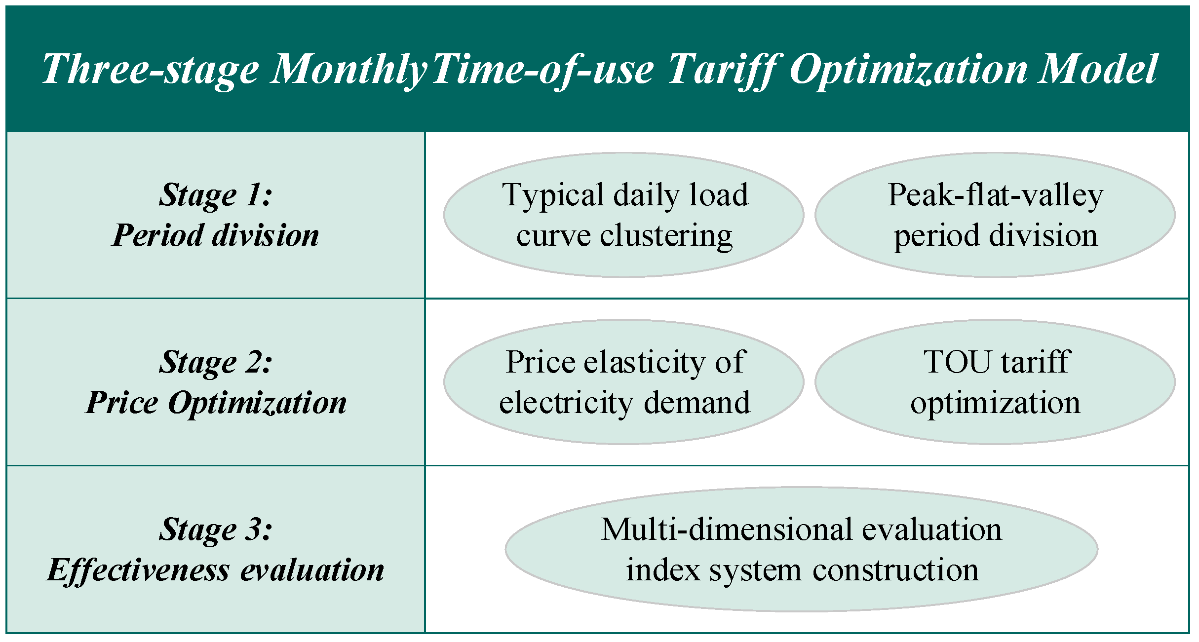
To fill the gap of the previous studies and existing practices, a three-stage monthly TOU tariff optimization model is constructed in this paper, and the framework is shown in Figure 3. First, the monthly typical daily net load curve is clustered using the K-means++ algorithm, and moving boundary technology (MBT) is adopted to divide the time periods. Then, a TOU tariff optimization model is constructed based on the consumers’ price elasticity of electricity demand (PEED). Finally, a multi-dimensional evaluation index system is constructed to assess the effectiveness of TOU tariff implementation.
The following points make up the bulk of this paper’s contributions:
  • Rather than using a basic load curve, time period division and price optimization are based on the net load curve, which accomplishes joint consideration for the supply and demand.
  • The K-means++ algorithm is adopted to cluster the typical daily net load curve, which can enhance the clustering effect by 4.27–26.70% compared to that of the conventional K-means technique.
  • Compared to the earlier annual/seasonal models, the monthly TOU tariff optimization model designed in this paper has a finer particle size. Furthermore, critical peak and deep valley time periods have also been taken into account in order to adapt to the new power system with ever-higher penetration rates of renewable energy than those of the peak, flat, and valley time periods considered in the majority of the previous research.
The structure of this study is as follows: After the introduction, Section 2 introduces the methodology applied in this paper. Section 3 presents an empirical analysis, and Section 4 presents a discussion of the results. The conclusions are given in Section 5.

2. Methodology

2.1. K-Means++ Algorithm

The K-means algorithm is one of the most extensively used clustering techniques and is used in many different fields [27]. When conducting typical load curve clustering, fuzzy C-means, self-organized maps, and some improved K-means algorithms are also employed to some extent [28,29,30]. The effectiveness of clustering still depends on whether the initial clustering center selection is reasonable, even though these models have been largely improved from various perspectives [31]. In 2006, Arthur and Vassilvitskii introduced the K-means++ algorithm as a solution to the previously listed problems [32]. The principle of the K-means++ algorithm is to identify the cluster centers through probability distribution.
Prior to outlining the fundamental steps of the K-means++ technique, it is imperative to elucidate the clustering criteria. As said in the preceding section, the majority of the existing studies concentrate on the demand side and use the load data as a clustering criterion, ignoring the power side’s renewable generation. In order to take into account the two sides in a synergistic manner, we cluster the typical daily curves using the net load rather than the traditional load data, as follows:
n l t = l t r g t
where n l t represents the net load at time t , l t represents the load at time t , and r g t represents the generation of renewable energy (the unity of wind power and photovoltaics are considered as renewable energy sources) at time t .
The steps of the K-means++ algorithm are shown as follows:
  • Step 1: Randomly choose the first cluster center δ 1 from the net load data N L = { n l 1 , n l 2 , , n l 24 } .
  • Step 2: Calculate the distance λ ( n l ) from each net load curve to the initial cluster center δ 1 .
  • Step 3: Set other cluster centers based on the probability ζ ( n l ) that each net load curve will be selected as the next cluster center (the net load curve with the maximum probability value). The calculation of probability ζ ( n l ) is as follows:
    ζ ( n l ) = λ ( n l ) 2 l L λ ( n l ) 2
  • Step 4: Repeat the above steps until k cluster centers are obtained.
The prior research primarily created a seasonal or annual TOU tariff, so that k = 1 or k = 4 in these studies. In order to propose a more refined dynamic electricity price optimization mechanism, this paper designs a monthly TOU tariff optimization model. Consequently, k = 12 in this paper. For more details, please consult Ref. [32].

2.2. MBT Approach

Even though easy to operate, the time period division method that splits the data into equal proportions in the previous studies diverges from reality and could lead to irrational TOU tariff optimization outcomes. Hence, we apply the MBT approach suggested by Yang et al. to realize time period division [33]. The MBT approach’s basic idea is to minimize the maximum distance inside each time period and maximize the minimum distance between various time periods [34]. The steps are as follows:
min F B c p , B p f , B f v , B v d = 1 24 m c , p , f , v , d t 24 n l t n l ¯ m 2
where m represents the five time periods designed in this paper (critical peak, peak, flat, valley, and deep valley), and n l ¯ m represents the average load of the m -th time period.
The steps of the MBT approach are shown as follows:
  • Step 1: Reconstruct the original typical daily net load curve in ascending order as N L = { n l 1 , n l 2 , , n l 24 } .
  • Step 2: Set initial boundaries as B c p = n l 1 , B p f = n l 2 , B f v = n l 3 , B v d = n l 4 and calculate the objective function F .
  • Step 3: Update the boundaries by moving forward a 1-h step, and calculate the objective function F again.
  • Step 4: Stop iteration and output the final result when t = 24 .
Apart from the utilization approach, the time period division model developed in this work differs significantly from the previous studies in two important ways:
  • The divided quantity of time periods. The previous studies mostly focused on three periods, i.e., the peak, flat, and valley periods, while this paper has expanded this to five periods.
  • The criteria for splitting time periods. Unlike earlier time period division based on the load data, we also use the net load as the primary foundation for time period division, which is similar to typical daily curve clustering.
For more details, please consult Ref. [33].

2.3. PEED Matrix

The PEED matrix is a key criterion reflecting the price–demand sensitivity of the users, which is widely applied in TOU tariff optimization fields [35]. Generally, the PEED can be divided into the self-elasticity and cross-elasticity coefficients [36]. Of which, the former reflects the impact of the current electricity price adjustment on the current power load, and the latter reflects the impact of electricity price adjustments at other times on the current power load.
ε t = l t / l t u t / u t ε t , h = l t / l t u h / u h
where ε ( t ) and ε ( t , h ) represent the self-elasticity coefficient and cross-elasticity coefficient, and u ( t ) and u ( h ) represent the electricity price at time t and h .
Hence, the power load after adjusting the electricity price can be expressed as follows:
l t = l t 0 1 + ε t u t u t 0 u t 0 + h = 1 h t 24 ε t , h u h u h 0 u h 0
where l 0 ( t ) represents the original load before electricity price adjustment at time t , and u 0 ( t ) and u 0 ( h ) , respectively, represent the original tariff before electricity price adjustment at time t and h .
Similar to the previous time period division section, we construct a [5 × 5]-dimension PEED matrix instead of the prior [3 × 3]-dimension matrix.

2.4. TOU Tariff Optimization Model

2.4.1. Objective Function

To achieve the “peak-cutting” and “valley-filling” effect by collaborative consideration of renewable energy generation characteristics, the following equation is constructed based on Equation (1), as follows:
min F = n l t , max n l t , min
where n l t , max and n l t , min represent the maximum and minimum net load, respectively.

2.4.2. Constraints

  • Cost constraints
For the power users, the electricity cost after the electricity price adjustment should not exceed the previously paid electricity cost, as shown in Equation (7):
t = 1 24 [ l t × u t ] t = 1 24 [ l t 0 × u t 0 ]
  • Tariff constraints
The electricity prices at different time periods have the following relationships:
u c > u p > u f > u v > u d
where the subscripts c , p , f , v , d represent the corresponding time periods of critical peak, peak, flat, valley, and deep valley.
  • Power constraints
The total electricity demand of users remains consistent before and after the electricity price adjustment, as follows:
t = 1 24 l t = t = 1 24 l t 0
In addition, there should be no peak–valley inversion after the load adjustment:
n l c > n l p > n l f > n l v > n l d

2.5. The Effectiveness Evaluation Index System of the TOU Optimization

To assess the superiority of the TOU tariff optimization model framework designed in this paper, an evaluation index system is constructed from the following aspects:
  • Economic characteristic indicators
From the perspective of economic characteristics, we mainly focus on the net load cost (I1), as follows:
N L C = t = 1 24 n l t × u t
where N L C represents the net load cost.
  • Load characteristic indicators
From the demand side perspective, the analysis is mainly based on indicators such as maximum load (I2), minimum load (I3), peak–valley difference (I4), and peak–valley difference rate (I5), as follows:
P V D = l t , max l t , min P V D R = ( l t , max l t , min ) / l ¯ t
where P V D and P V D R represent the corresponding peak–valley difference and peak–valley difference rate, respectively.
  • Generation characteristic indicators
The TOU tariff optimization model designed in this paper can not only suppress the fluctuation of power load but also reduce the waste of renewable energy. Therefore, the abandonment of renewable energy (I6) is chosen as follows:
R E A = t = 1 24 r e a t r e a t = n l t n l t 0   0 n l t > 0
where R E A represents the abandonment of renewable energy.
Hence, the index system is constructed based on the indicators above, as shown in Figure 4.
As shown in Figure 4, the indicators above can be divided into two types: cost-type indicators and benefit-type indicators. Of which, the former involves the smaller, the better, and the latter involves the larger, the better.

3. Empirical Analysis

3.1. The Basic Information

To verify the applicability and superiority of the three-stage TOU tariff optimization model developed in this paper, we conduct an empirical analysis of real data from a northwest province in China. This province has exceptional wind and solar resources as a result of its geographic location, which results in a large potential for producing renewable energy generation. To create a monthly TOU tariff, we first gather the bilateral supply and demand data for the entire province in 2022. Figure A1, Figure A2 and Figure A3 show the hourly power load, wind generation, and photovoltaic generation curves. Then, the hourly net load data are further computed, as shown in Figure 5.
The time period division and price settings in the province are shown in Table 3.
Table 3 illustrates that this province solely applies one set of TOU tariffs throughout the year, making it unable to adjust to the constantly shifting features of power generation and load. Furthermore, the province only implements three time periods: the peak, flat, and valley, which is ineffective at mitigating grid congestion during critical peak hours or the squandering of renewable energy during deep valley periods.

3.2. Clustering of the Typical Daily Net Load Curve

To design a monthly TOU tariff, we cluster the typical daily net load curve of each month. Considering the space limitations, only the clustering processes in January and February are shown in Figure 6, and the clustering results of each month are listed in Figure A4.

3.3. Division of the Time Periods

Based on the MBT approach introduced in Section 2.2, the time periods of each month are divided, as listed in Figure 7.
Due to the large-scale generation of renewable energy, the net load during the afternoon period is relatively low and can be set as valley or deep valley periods. On the contrary, due to the low-level power generation of photovoltaics at night, the net load at night is relatively high and can be set as peak periods or critical peak periods.

3.4. TOU Optimization Results

Due to the fact that the region currently only implements the TOU tariff for the peak, flat, and valley periods, there is a deviation from the five time periods of the TOU tariff designed in this paper. The lack of electricity prices in the critical peak and deep valley periods will lead to the incompleteness of the PEED matrix. Therefore, based on the existing research, we set the electricity price during the critical peak hours to 1.2 times more than that during the peak hours and set it during the deep valley hours to 0.8 times more than that during the valley hours. Then, the PEED matrix is constructed as follows:
P E E D = 0.2598 0.2560 0.3010 0.4509 0.4582 0.2560 0.2316 0.2734 0.4145 0.4197 0.3010 0.2734 0.2507 0.3819 0.3866 0.4509 0.4145 0.3819 0.3927 0.3985 0.4582 0.4197 0.3866 0.3985 0.3878
Based on the PEED matrix, the TOU tariff is optimized using the TOU optimization model proposed in Section 2.4, as shown in Table 4. In addition, the optimized load is listed in Figure A5.

3.5. Effectiveness Evaluation

To verify the effectiveness of the proposed three-stage monthly TOU tariff optimization model, the effectiveness is evaluated using the index system presented in Section 2.5, as shown in Table 5.

4. Discussion

4.1. Clustering Effect Comparison

To prove the superiority of the K-means++ algorithm proposed in this paper, the clustering effect is compared to the traditional K-means algorithm through the sum of squared errors criterion (SSE). The calculation for the SSE is presented in Equation (14), and the comparison results are listed in Table 6.
ξ S S E = k = 1 K α ρ k α δ k 2
where α is the point belonging to the cluster ρ .
As shown in Table 6, the clustering effect of the K-means++ algorithm is better than that of the K-means algorithm for all the months, and the SSE value decreased by 4.27–26.70% (4.27% in August and 26.70% in December).

4.2. Time Period Division Comparison

In order to demonstrate the superiority of the time period division proposed in this paper, we conduct a comparison. In this scenario, we still use the typical daily net load data clustered in this paper. However, 24 h is set into three time periods: the peak, flat, and valley, as in the previous studies. The time period division results are shown in Figure 8.
As shown in Figure 8, the division results of the flat time periods based on the traditional criterion are similar to the time period division results designed in this paper. However, the peak and valley time periods are further split apart.

4.3. TOU Tariff Optimization Comparison

In order to verify the superiority of the three-stage TOU tariff optimization framework designed in this paper, we conduct a comparative analysis of two aspects.

4.3.1. Comparison with the Effectiveness before Optimization

Table 7 depicts the effectiveness evaluation without applying the TOU tariff optimization model, and the evaluation indicators still follow the effectiveness evaluation index system constructed in Section 2.5.
As shown in Table 7, the proposed TOU tariff optimization model performs well in terms of the economy, load, and generation characteristics. Considering the economic characteristics, the electricity cost before optimization ranges from CNY 69,192 to CNY 113,189, while the electricity cost after optimization ranges from CNY 65,207 to CNY 101,128. Considering the load characteristics, the peak–valley difference before optimization ranges from 5661 MW to 9472 MW, while the peak–valley difference after optimization ranges from 3008 MW to 9126 MW (taking the peak–valley difference as an example). Considering the generation characteristics, the abandonment of renewable energy before optimization ranges from 0 MW to 1900 MW, while the abandonment of renewable energy after optimization ranges from 0 MW to 282 MW.

4.3.2. Comparison with the Effectiveness Based on Three Traditional Time Periods

Table 8 presents the effectiveness evaluation using the conventional three-time-period approach, with Section 4.2 representing the division criterion. In fact, this scenario only compares and analyzes the effects of different time periods. Hence, the typical net load curve has not been altered and indicators like I2 to I6 have not changed directly. For this purpose, we mainly compare the changes in the net load costs (I1) using different time period division rules.
With the exception of August, the consumers’ monthly electricity consumption costs are lower under the TOU tariff optimization framework created in this study than those under the three conventional time periods. In general, the power consumers modify their electricity consumption behavior to achieve larger profits than they could in the traditional peak–flat–valley time periods after adding the critical peak and deep valley time periods. Using the province’s 2022 data as an example, the overall net load cost dropped by 10.36%, with February seeing the biggest drop in costs at 19.16%.

5. Conclusions

As an important component of the future power system, the uncertainty of renewable energy generation will inevitably affect the safe and stable operation of the power system, and the users’ DR is the key means to address this issue. As one of the main price-based DRs, the design of a TOU tariff has gained plenty of attention in practice and research. However, the unclear time period division, unreasonable price setting, and incomplete seasonal factor consideration restrict the development of the TOU to some extent. To address the aforementioned issues, we constructed a three-stage monthly optimization model in this paper. The following conclusions were obtained:
  • As it is different from the previous clustering models, the adopted K-means++ algorithm can overcome the impact of improper selection of initial clustering centers, with an error reduction of 4.27–26.70%. Furthermore, the consideration of the renewable energy generation introduces a more reasonable time period division standard.
  • In addition to considering the net load, more extensive and adaptable time division criteria have been proposed to adapt to the increasing penetration rate of renewable energy. Comparing to the three traditional time periods, this paper further introduces the critical peak and deep valley time periods, which enabled a cost saving of 10.36% of the net load cost reduction.
  • Using the three-stage monthly TOU tariff optimization model, the monthly net load cost decreased by 2.03–17.27%, the peak–valley difference decreased by 0.31–53.94%, and the maximum monthly abandonment of renewable energy decreased by 1900 MW.
With the continuous construction of new power systems, the introduction of multiple loads with unpredictable behavior patterns exacerbates the uncertainty of the users, and the intermittency and volatility of renewable energy generation will eventually result in a significant power supply and asynchrony. Through this study, we strove to find a new path to lead demand side development. Following the aforementioned results, several suggestions are further presented:
  • We must develop more rigorous and extensive time period division methods. With the increase in the installed capacity and penetration rate of renewable energy, the applicability of research based on peak–flat–valley time periods has significantly diminished. In addition, the time periods should not be fixed and evenly divided, which is inconsistent with the actual characteristics of the users and power sources.
  • We must develop a reasonable price difference between each time period. At present, the unreasonable TOU tariff has, to some extent, led to the problem of users’ unwillingness to respond. Therefore, it is necessary to further design a users’ response willingness representation model (such as the consumer psychology and PEED matrix ones) and propose more scientific and reasonable electricity price optimization methods.
  • We must develop dynamic and comprehensive price adjustment and feedback mechanisms. There is a significant time-varying characteristic in the electricity load and power generation. The traditional electricity pricing mechanisms mostly have annual adjustment cycles, with only a few with quarterly adjustment cycles. In the future, the dynamic adjustment of electricity prices should be more frequent and adapt to the actual demand.
The limitations and future directions are presented as follows:
  • As analyzed in Section 1.2, different regions implement different TOU tariffs. The time period and price setting are quite different due to resource endowment and user composition. Considering the data limitations, we only took a northwestern province as an example, which should be further expanded to include more regions in the future.
  • Although most regions design a TOU tariff for the entire industry, some regions also attempt to break down some typical industries. In the future, we will screen some typical industries (such as those with a high load proportion and strong adjustability) for separate TOU tariff designs.

Author Contributions

Conceptualization, H.Z. (Hailang Zhou) and H.W.; methodology, P.Y. and S.L.; software, Y.Z.; validation, H.Z. (Huiru Zhao); resources, C.L. and C.Z.; writing—original draft preparation, Y.Z.; writing—review and editing, H.Z. (Huiru Zhao); visualization, Y.Z.; supervision, P.Y., S.L., C.L. and C.Z.; project administration, H.Z. (Hailang Zhou) and H.W. All authors have read and agreed to the published version of the manuscript.

Funding

This research was funded by the project “Research on the Evaluation and Pricing Technology of the Interactive Response of Power Demand Side Resources under the Transformation of Price Reform” of the Science and Technology Project of the State Grid Corporation of China (SGCQKH00SCJS2250078).

Data Availability Statement

The data presented in this study are available on request from the corresponding author. The data are not publicly available due to privacy.

Acknowledgments

The authors are grateful to the editor and anonymous reviewers for their work.

Conflicts of Interest

Authors Peipei You, Sitao Li, Chengren Li and Chao Zhang have received research grants from State Grid Energy Research Institute Co., Ltd. Authors Hailang Zhou and Huicai Wang have received research grants from Marketing Service Center of State Grid Chongqing Electric Power Company.

Appendix A

Figure A1. The hourly load curve of a Chinese province in 2022.
Energies 16 07858 g0a1
Figure A2. The hourly wind generation curve of a Chinese province in 2022.
Energies 16 07858 g0a2
Figure A3. The hourly photovoltaic generation curve of a Chinese province in 2022.
Energies 16 07858 g0a3
Figure A4. The typical daily net load of each month (initial).
Energies 16 07858 g0a4
Figure A5. The typical daily net load of each month (optimized).
Energies 16 07858 g0a5

References

  1. Zhao, Y.; Su, Q.; Li, B.; Zhang, Y.; Wang, X.; Zhao, H.; Guo, S. Have those countries declaring “zero carbon” or “carbon neutral” climate goals achieved carbon emissions-economic growth decoupling? J. Clean. Prod. 2022, 363, 132450. [Google Scholar] [CrossRef]
  2. Wang, S.; Li, F.; Zhang, G.; Yin, C. Analysis of energy storage demand for peak shaving and frequency regulation of power systems with high penetration of renewable energy. Energy 2023, 267, 126586. [Google Scholar] [CrossRef]
  3. Liu, Z.; Zhao, S.; Zhang, X.; Tang, Y.; You, G.; Li, J.; Zhao, S.; Hou, X. Renewable energy utilizing and fluctuation stabilizing using optimal dynamic grid connection factor strategy and artificial intelligence-based solution method. Renew. Energy 2023, 219, 119379. [Google Scholar] [CrossRef]
  4. Wu, Z.; Chen, L.; Wang, J.; Zhou, M.; Li, G.; Xia, Q. Incentivizing the Spatiotemporal Flexibility of Data Centers Toward Power System Coordination. IEEE Trans. Netw. Sci. Eng. 2023, 10, 1766–1778. [Google Scholar] [CrossRef]
  5. Chen, Y.; Li, J.; Li, H. Tradeoffs in cost competitiveness and emission reduction within microgrid sustainable development considering price-based demand response. Sci. Total Environ. 2020, 73, 135545. [Google Scholar] [CrossRef] [PubMed]
  6. Zheng, S.; Sun, Y.; Li, B.; Qi, B.; Shi, K.; Li, Y.; Du, Y. Bargaining-based cooperative game among multi-aggregators with overlapping consumers in incentive-based demand response. IET Gener. Transm. Distrib. 2020, 14, 1077–1090. [Google Scholar] [CrossRef]
  7. McKenna, K.; Keane, A. Residential Load Modeling of Price-Based Demand Response for Network Impact Studies. IEEE Trans. Smart Grid 2016, 7, 2285–2294. [Google Scholar] [CrossRef]
  8. Grimm, V.; Orlinskaya, G.; Schewe, L.; Schmidt, M.; Zöttl, G. Optimal design of retailer-prosumer electricity tariffs using bilevel optimization. Omega 2021, 102, 102327. [Google Scholar] [CrossRef]
  9. Choi, D.; Murali, K. The impact of heterogeneity in consumer characteristics on the design of optimal time-of-use tariffs. Energy 2022, 254, 124248. [Google Scholar] [CrossRef]
  10. Li, R.; Wang, Z.; Gu, C.; Li, F.; Wu, H. A novel time-of-use tariff design based on Gaussian Mixture Model. Appl. Energy 2016, 162, 1530–1536. [Google Scholar] [CrossRef]
  11. Yuan, X.; Cai, Q.; Song, D. Power Consumption Behavior Analysis Based on Cluster Analysis. In Proceedings of the International Symposium on Artificial Intelligence and Robotics 2021, Shenzhen, China, 25–26 April 2021; Volume 11884, p. 2605823. [Google Scholar]
  12. Liu, F.; Dong, T.; Hou, T.; Liu, Y. A Hybrid Short-Term Load Forecasting Model Based on Improved Fuzzy C-Means Clustering, Random Forest and Deep Neural Networks. IEEE Access 2021, 9, 59754–59765. [Google Scholar] [CrossRef]
  13. Li, M.; Xu, D.; Zhang, D.; Zou, J. The seeding algorithms for spherical k-means clustering. J. Glob. Optim. 2020, 76, 695–708. [Google Scholar] [CrossRef]
  14. He, Y.; Ye, Z.; Wei, W. Research on time division of peak-valley tou tariff considering price elasticity of user demand. Prices Mon. 2022, 12, 1–9. [Google Scholar]
  15. Bai, X.; Zhang, R.; Xu, L. Research on optimization strategy of time-of-use electricity price for e-commerce sales under the background of electricity reform—Analysis considering user-side and price-based demand response. Price Theory Pract. 2021, 10, 54–57+193. [Google Scholar]
  16. Gou, J.; Lin, C.; Li, J.; Geng, B.; Li, Z.; Cao, Y.; Bao, Y. Charging Strategy for Electric Vehicles Considering Consumer Psychology and Trip Chain. Front. Energy Res. 2021, 9, 723370. [Google Scholar] [CrossRef]
  17. Andruszkiewicz, J.; Lorenc, J.; Weychan, A. Seasonal variability of price elasticity of demand of households using zonal tariffs and its impact on hourly load of the power system. Energy 2020, 196, 117175. [Google Scholar] [CrossRef]
  18. Gholizadeh-Roshanagh, R.; Zare, K. Electric power distribution system expansion planning considering cost elasticity of demand. IET Gener. Transm. Distrib. 2019, 13, 5229–5238. [Google Scholar] [CrossRef]
  19. Yang, H.; Wang, L.; Ma, Y.; Zhang, D.; Wu, H. Optimization strategy of price-based demand response considering the bidirectional feedback effect. IET Gener. Transm. Distrib. 2021, 15, 1752–1762. [Google Scholar] [CrossRef]
  20. Zhang, J.; Zhang, Q.; Li, G.; Wu, J.; Wang, C.; Li, Z. Hybrid Model for Renewable Energy and Load Forecasting Based on Data Mining and EWT. J. Electr. Eng. Technol. 2022, 17, 1517–1532. [Google Scholar] [CrossRef]
  21. de Sá Ferreira, R.; Barroso, L.A.; Lino, P.R.; Carvalho, M.M.; Valenzuela, P. Time-of-Use Tariff Design Under Uncertainty in Price-Elasticities of Electricity Demand: A Stochastic Optimization Approach. IEEE Trans. Smart Grid 2013, 4, 2285–2295. [Google Scholar] [CrossRef]
  22. Taik, S.; Kiss, B. Clustering-based Optimal Dynamic Pricing for Residential Electricity Consumers. In Proceedings of the 23rd International Conference on Process Control (PC), Strbske Pleso, Slovakia, 1–4 June 2021; pp. 143–148. [Google Scholar]
  23. Bian, S.; Wang, Z.; Song, W.; Zhou, X. Feature extraction and classification of time-varying power load characteristics based on PCANet and CNN+Bi-LSTM algorithms. Electr. Power Syst. Res. 2023, 217, 109149. [Google Scholar] [CrossRef]
  24. Venizelou, V.; Philippou, N.; Hadjipanayi, M.; Makrides, G.; Efthymiou, V.; Georghiou, G.E. Development of a novel time-of-use tariff algorithm for residential prosumer price-based demand side management. Energy 2018, 142, 633–646. [Google Scholar] [CrossRef]
  25. Samadi, M.; Aghamohamadi, M.; Mahmoudi, A. Optimal time period clustering of time-of-use schemes based on elastic loads’ responsiveness. Int. Trans. Electr. Energy Syst. 2020, 30, e12275. [Google Scholar] [CrossRef]
  26. Xue, W.; Zhao, X.; Li, Y.; Mu, Y.; Tan, H.; Jia, Y.; Zhao, Y. Research on the Optimal Design of Seasonal Time-of-Use Tariff Based on the Price Elasticity of Electricity Demand. Energies 2023, 16, 1625. [Google Scholar] [CrossRef]
  27. Ahmed, M.; Seraj, R.; Islam, S. The k-means Algorithm: A Comprehensive Survey and Performance Evaluation. Electronics 2020, 9, 1295. [Google Scholar] [CrossRef]
  28. Dedić, A.; Konjić, T.; Ćalasan, M.; Dedić, Z. Fuzzy C-Means Clustering Applied to Load Profiling of Industrial Customers. Electr. Power Compon. Syst. 2022, 49, 1068–1084. [Google Scholar] [CrossRef]
  29. Tsekouras, G.; Hatzilau, I.; Prousalidis, J. A new pattern recognition methodology for classification of load profiles for ships electric consumers. J. Mar. Eng. Technol. 2009, 14, 45–58. [Google Scholar] [CrossRef]
  30. Tsekouras, G.J.; Kotoulas, P.B.; Tsirekis, C.D.; Dialynas, E.N.; Hatziargyriou, N.D. A pattern recognition methodology for evaluation of load profiles and typical days of large electricity customers. Electr. Power Syst. Res. 2008, 78, 1494–1510. [Google Scholar] [CrossRef]
  31. Sinaga, K.; Yang, M. Unsupervised K-Means Clustering Algorithm. IEEE Access 2020, 8, 80716–80727. [Google Scholar] [CrossRef]
  32. Arthur, D.; Vassilvitskii, S. K-Means++: The Advantages of Careful Seeding. In Proceedings of the Eighteenth Annual ACM-SIAM Symposium on Discrete Algorithms, SODA 2007, New Orleans, LA, USA, 7–9 January 2007. [Google Scholar]
  33. Yang, H.; Wang, L.; Zhang, Y.; Tai, H.M.; Ma, Y.; Zhou, M. Reliability Evaluation of Power System Considering Time of Use Electricity Pricing. IEEE Trans. Power Syst. 2019, 34, 1991–2002. [Google Scholar] [CrossRef]
  34. Yang, H.; Wang, L.; Ma, Y. Optimal Time of Use Electricity Pricing Model and Its Application to Electrical Distribution System. IEEE Access 2019, 7, 123558–123568. [Google Scholar] [CrossRef]
  35. Andruszkiewicz, J.; Lorenc, J.; Weychan, A. Demand Price Elasticity of Residential Electricity Consumers with Zonal Tariff Settlement Based on Their Load Profiles. Energies 2019, 12, 4317. [Google Scholar] [CrossRef]
  36. Zhai, Z.; Zhang, L.; Hou, X.; Yang, Q.; Huang, Z. Price elasticity of electricity demand in China A new instrument variable based on marketization policy. Energy Sustain. Dev. 2023, 76, 101275. [Google Scholar] [CrossRef]
Figure 1. The main components of FRs in a power system.
Energies 16 07858 g001
Figure 2. The main components of IDR and PDR.
Energies 16 07858 g002
Figure 3. The framework of the three-stage monthly TOU tariff optimization model.
Energies 16 07858 g003
Figure 4. The effectiveness evaluation index system of the TOU optimization.
Energies 16 07858 g004
Figure 5. The hourly net load curve of a Chinese province in 2022.
Energies 16 07858 g005
Figure 6. The clustering process of January and February. Note: The grey lines represent the net load curves of the corresponding month, and the red line represents the typical daily net load curve clustered using the K-means++ algorithm.
Energies 16 07858 g006
Figure 7. The time period division of each month.
Energies 16 07858 g007
Figure 8. The time period division of each month (three time periods).
Energies 16 07858 g008
Table 1. The time period division and seasonal setting in California and New South Wales.
RegionSeasonPeakFlatValley
CaliforniaSummer (1 May to 31 October)12:00–18:008:30–12:00, 18:00–21:3021:30–8:30
Winter (1 November to 30 April)/8:30–9:3021:30–8:30
New South WalesSummer (1 June to 31 August)17:00–21:007:00–17:00, 21:00–22:0022:00–7:00
Winter (1 November to 31 March)14:00–20:007:00–14:00, 20:00–22:022:00–7:00
Other seasons14:00–20:007:00–14:00, 20:00–22:022:00–7:00
Noted: Although the time period division of winter and other seasons in New South Wales is the same, they have different tariff settings.
Table 2. The implementation of TOU tariff in 31 regions in China as of November 2022.
RegionPeak–Valley Tariff RatioCritical Peak TariffDeep Valley TariffSeasonal Tariff
Beijing4:1
Tianjin3.26:1
Northern Hebei3:1
Southern Hebei5.67:1
Shanxi3.56:1
Shandong5.67:1
Henan2.78:1
Hubei2.87:1
Hunan4:1
Sichuan4:1
Chongqing4.21:1
Jiangxi3:1
Jiangsu4.11:1
Shanghai3.2:1
Zhejiang3.57:1
Anhui4.15:1
Fujian4:1
Heilongjiang3:1
Jilin3:1
Inner Mongolia3:1
Liaoning3:1
Shannxi3:1
Gansu3:1
Ningxia3:1
Qinghai4.21:1
Xinjiang4.71:1
Guangdong4.47:1
Guangxi3:1
Guizhou3:1
Hainan4.25:1
Yunnan3:1
Note: Hebei province is divided into two regions: Northern Hebei and Southern Hebei, because they are governed by different power grid enterprises. “√” represents that the region implements the corresponding type of tariff.
Table 3. The time period division and price settings in the province.
PeakFlatValley
Time period division (hours)8:00–10:00
18:00–22:00
11:00–17:00
23:00
0:00–7:00
Tariff (CNY/MWh)0.76180.43040.1808
Table 4. The TOU tariff of each period in each month.
Critical PeakPeakFlatValleyDeep Valley
January0.68760.43990.28080.2340.1872
February0.6470.50680.28540.23780.1902
March0.85510.71770.37740.31450.2516
April0.68270.66050.56320.32660.2612
May0.79280.66070.34820.29020.2321
June0.69680.58070.32020.26680.2134
July0.68470.57530.35340.29450.2356
August0.80860.76490.75870.31060.1887
September0.6810.56750.32320.26930.2154
October0.68850.52120.49310.23490.1879
November0.68850.59360.44450.29510.2361
December0.6980.6630.31120.25930.2075
Table 5. The effectiveness evaluation of the TOU tariff optimization model.
MonthI1 (CNY)I2 (MW)I3 (MW)I4 (MW)I5I6 (MW)
January96,452922397912698.95%0
February78,675868508685100.00%0
March74,8047595−1327727101.74%282
April65,580723407234100.00%0
May65,20775023153434957.97%0
June76,14075992628497165.42%0
July78,0938152536761693.42%0
August78,35061713163300848.75%0
September84,75985671959660877.13%0
October100,20692952188710776.46%0
November97,8519159638852193.04%0
December101,1289258675858392.70%0
Table 6. The comparison results of the clustering effect.
K-Means++K-Means
ξ S S E J a n 5.07 × 1085.92 × 108
ξ S S E F e b 5.65 × 1086.70 × 108
ξ S S E M a r 6.52 × 1087.13 × 108
ξ S S E A p r 5.83 × 1086.43 × 108
ξ S S E M a y 3.32 × 1084.11 × 108
ξ S S E J u n 4.11 × 1084.38 × 108
ξ S S E J u l 6.27 × 1087.18 × 108
ξ S S E A u g 6.06 × 1086.33 × 108
ξ S S E S e p 5.74 × 1086.08 × 108
ξ S S E O c t 6.44 × 1086.97 × 108
ξ S S E N o v 5.40 × 1086.41 × 108
ξ S S E D e c 5.71 × 1087.79 × 108
Table 7. The effectiveness evaluation without applying the TOU tariff optimization model.
MonthI1 (CNY)I2 (MW)I3 (MW)I4 (MW)I5I6 (MW)
January109,4189465120934598.73%0
February95,0949007−4659472105.16%1622
March80,1468872−1899061102.13%404
April69,1928196−4878683105.94%1900
May78,40084692808566166.84%0
June86,62684411952648976.87%0
July86,2638421782764090.72%0
August81,97781491618653080.14%0
September96,05389421674726881.28%0
October113,18997351267846886.99%0
November107,7299510800871091.59%0
December103,2199856563929394.29%0
Table 8. The effectiveness evaluation based on three traditional time periods.
MonthI1 (CNY) in Five Time PeriodsI1 (CNY) in Three Time Periods
January96,452110,712
February78,67597,320
March74,80481,609
April65,58074,369
May65,20778,837
June76,14080,067
July78,09382,875
August78,35075,566
September84,75997,592
October100,206106,547
November97,851112,245
December101,128114,737
Sum997,2451,112,476
Disclaimer/Publisher’s Note: The statements, opinions and data contained in all publications are solely those of the individual author(s) and contributor(s) and not of MDPI and/or the editor(s). MDPI and/or the editor(s) disclaim responsibility for any injury to people or property resulting from any ideas, methods, instructions or products referred to in the content.

