Pore-Scale Modeling of Methane Hydrate Dissociation Using a Multiphase Micro-Continuum Framework

Abstract

The development of methane hydrate extraction technology remains constrained due to the limited physical understanding of hydrate dissociation dynamics. While recent breakthroughs in pore-scale visualization techniques offer intuitive insights into the dissociation process, obtaining a profound grasp of the underlying mechanisms necessitates more than mere experimental observations. In this research, we introduce a two-phase micro-continuum model that facilitates the numerical simulation of methane hydrate dissociation at both single- and multiscale levels. We employed this numerical model to simulate microfluidic experiments and determined the kinetic parameters of methane hydrate dissociation based on experimental data under various dissociation scenarios. The simulations, once calibrated, correspond closely to experimental results. By comprehensively comparing the simulated results with experimental data, the rate constant and the effective diffusion coefficient were reliably determined to be k_d = 1.5 × 10⁸ kmol²/(J·s·m²) and D_l = 0.8 × 10⁻⁷ m²/s, respectively. Notably, the multiscale model not only matches the precision of the single-scale model but also presents considerable promise for streamlining the simulation of hydrate dissociation across multiscale porous media. Moreover, we contrast hydrate dissociation under isothermal versus adiabatic conditions, wherein the dissociation rate is significantly reduced under adiabatic conditions due to the shifted thermodynamic condition. This comparison highlights the disparities between microfluidic experiments and real-world extraction environments.

1. Introduction

Addressing global warming and energy shortages necessitates the adoption of clean and efficient energy alternatives to traditional fossil fuels. Methane hydrates have risen to prominence as an alternative energy source due to their vast gas storage capacity [1] and abundant reserves [2]. Remarkably, methane hydrate reserves are estimated to surpass the combined total of all other fossil fuels on Earth [3,4]. This potential has garnered significant global interest. The development of a broad range of applications for gas-hydrate-based technologies has also increased research attention in this field, including CO₂ capture and storage, water desalination, and energy storage [5]. Methane hydrates are crystalline structures wherein methane molecules are housed within hydrogen-bonded lattices via intermolecular forces [6]. Their stability demands low-temperature and high-pressure conditions, leading to their distribution in deep-sea sediments and terrestrial permafrost. To extract methane from hydrates, methods like thermal stimulation [7], depressurization [8], and inhibitor injection [9] have been tested, all aiming to disturb the thermodynamic balance of hydrates. Among these mining methods, depressurization has a higher mining efficiency and is considered the most promising mining option. However, given varying reservoir conditions and intricate dissociation mechanisms, the methane hydrate extraction efficiency remains constrained, leaving many nations in the preliminary exploration phase. As a result, there is still a need for a deeper understanding of the hydrate decomposition mechanism to improve mining operations.

Methane hydrate dissociation is a typical multiscale and multi-physical process and involves complicated multiphase heat and mass transfer phenomena within sediment pore structures [10]. Therefore, investigations on methane hydrate dissociation should be carried out at multiple scales, including the field scale [11], laboratory scale [12,13,14,15], and pore scale [16,17]. Among these works, pore-scale studies provide a more detailed understanding of the dissociation mechanisms by penetrating the comprehensive process occurring within the porous structure. With the continuous development of experimental techniques, pore-scale experimental studies of methane hydrate dissociation have been carried out in recent years, including micro-CT imaging and microfluidic experiments. These experimental studies analyze the hydrate dissociation mechanisms by observing the evolution of gas, water, and hydrate phases during hydrate dissociation. In particular, microfluidic experiments offer superior spatial and temporal resolutions. Ever since their introduction by Tohidi et al. [18] for studying gas hydrate formation and dissociation, their prevalence has grown. Such experiments have enhanced our understanding of dissociation via depressurization. For instance, Katsuki et al. [19] noted that small-bubble coalescence creates continuous gas slugs, expediting hydrate dissociation. Almenningen et al. [20] showed that dissociation is quicker in the presence of free gas and slower when water is encased. Farahani et al. [21] presented a coupled geophysical–geothermal scheme for the quantification of hydrates in gas-hydrate-bearing permafrost sediments, which are sensitive to hydrate saturation and the pore-scale habit. These findings shed light on fluid dynamics’ role in hydrate dissociation. However, solely relying on experimental observations can be limiting. Pore-scale numerical simulations remain crucial for a deeper comprehension of the dissociation mechanism.

As computational technology has advanced, pore-scale numerical studies on methane hydrate dissociation have become more prevalent. Jeong et al. [22] established a pore-scale model for estimating the dissociation rate of CO₂ hydrate using the finite volume method (FVM) with 3D unstructured mesh. Mohammadmoradi et al. [23] reconstructed distributions of fluid and hydrate and predicted the relative permeabilities using a direct pore morphological model. They found that the hydrate dissociation rates are primarily controlled by the intrinsic permeability, porosity, and water saturation and are barely affected by the relative permeabilities. Zhang et al. [24] developed a pore-scale model to simulate methane hydrate dissociation in a singular gas stream, finding the dissociation rate to be significantly influenced by heat transfer restrictions due to the endothermic nature of the reaction. Wang et al. [25,26] investigated the impact of ice formation and mass transfer constraints within the pore structure, incorporating both the heat and mass transfer of phase transitions in their models. To fully unravel the interaction between gas–water multiphase flow and interfacial mass transfer during dissociation, Yang et al. [10,27] conducted pore-scale simulations of multiphase reaction transport during dissociation. They underscored the significance of mass transfer restrictions on hydrate dissociation and presented a regime map to detail the multi-faceted interplay between heat and mass transfer. However, due to constraints on numerical models and computational resources, current pore-scale simulations can be challenging to align with experimental findings. A comprehensive quantitative validation remains elusive, underscoring the need for more refined pore-scale numerical models that facilitate a direct quantitative comparison with experimental results.

The micro-continuum Darcy–Brinkmann–Stokes (DBS) model was developed to simulate the reactive flow in porous media via single-field equations due to its ability to handle the dynamic evolution of the solid–fluid interface without a body-fitted mesh or re-meshing strategy. For example, Soulaine et al. [28] simulated the mineral dissolution of a single calcite crystal, and the results agreed with the classic arbitrary Lagrangian–Eulerian solver. Many numerical studies have demonstrated that the micro-continuum DBS framework is reliable in modeling single-phase reactive flows across multiscale porous media [28,29,30,31]. The multiphase micro-continuum model has also been developed in recent years. Horgue [32] and Soulaine [33] proposed two-phase micro-continuum DBS frameworks to describe the two-phase flow at both the pore and continuum scales. Carrillo [34] later improved the multiphase micro-continuum model with a theoretical derivation to asymptotically match the scale-dependent multiphase model, and Liu et al. proposed corrections to mitigate spurious velocities at the gas–liquid interface and contact-line regions [35]. Thanks to these efforts, the multiphase micro-continuum model shows the potential to simulate multiphase flow across multiscale porous media. In summary, the DBS model demonstrates a strong ability to simulate multiphase reactive flows in porous media, which is expected to enable numerical simulations of the hydrate dissociation process. However, the numerical model should be further developed by coupling the hydrate dissociation kinetics with the micro-continuum framework.

In this study, we conducted pore-scale numerical simulations of methane hydrate dissociation and compared the results with data from microfluidic experiments to validate the developed micro-continuum models. A multiscale simulation method for hydrate dissociation was developed based on the existing micro-continuum model, which can simultaneously solve hydrate dissociation problems through resolved micropores within the sediment and unresolved sub-micropores inside the hydrate and handle the hydrate evolution without a re-meshing strategy. By aligning the numerical and experimental outcomes, we can ascertain the kinetic parameters for methane hydrate dissociation. Additionally, we implemented multiscale modeling to show the capability of the numerical model to enhance computational efficiency without compromising accuracy. Finally, the hydrate dissociation dynamics under isothermal and adiabatic conditions were compared to understand the importance of heat transfer in predicting the dissociation rate.

2. Mathematical Models

In this section, the mathematical model based on the two-phase micro-continuum DBS framework is developed to simulate the methane hydrate dissociation process at both the resolved pore scale (macropores) and the unresolved Darcy scale (micropores), as shown in Figure 1.

2.1. Hydrate Dissociation Model

Methane hydrate begins to dissociate when the hydrate phase equilibrium is disturbed by either depressurizing or heating in hydrate-bearing sediments. The hydrate dissociation equation can be expressed as

$${\mathrm{CH}}_4\cdot n_{\mathrm{H}}{\mathrm{H}}_2\mathrm{O} \to {\mathrm{CH}}_4+n_{\mathrm{H}}{\mathrm{H}}_2{\mathrm{O}}_{(\mathrm{s})}, \Delta H>0$$

(1)

where $n_{\mathrm{H}}$ is the hydrate number (in this work, $n_{\mathrm{H}}=6$), and $\Delta H$ is the standard enthalpy of methane hydrate dissociation. It should be noted that the dissociation process is very complicated, as it involves the two-phase flow, heat and mass transfer, and hydrate evolution. Meanwhile, it is difficult to quantify the produced methane that diffuses into the bulk gas phase and particles that dissolve in the water due to supersaturation and micro- and nanobubbles. To ensure the numerical stability and computing efficiency, the following assumptions were made in this study: (1) the fluids are incompressible, and the non-slip boundary condition is enforced at the fluid–solid interface; (2) the produced methane is regarded as a dilute solution in water, the diffusion of methane molecules follows Fick’s law, and the concentration jump at the gas–water interface is described by Henry’s law; (3) dissociation preferentially occurs from the methane hydrate surface, and hydrate reformation and ice formation are neglected; (4) the fluid and solid physical properties are assumed to be constant, and the buoyancy force is neglected.

As the dissociation process can be induced by different methods, such as depressurization, raised temperature, and amalgamative changes in pressure and temperature, the dissociation flux of methane hydrate is determined by Sean’s rate equation [36] as follows:

$$F_{{\mathrm{CH}}_4}=k_{\mathrm{d}}\exp (-\frac{\Delta E}{T})RT\ln \frac{x_{\mathrm{R}}}{x_{\mathrm{S}}}$$

(2)

where $k_d$ is the rate constant, $\Delta E$ is the activation energy, $R$ is the ideal gas constant, $T$ is the dissociation temperature, $x_{\mathrm{S}}$ is the local solubility of methane in the aqueous solution, and $x_{\mathrm{R}}$ is the solubility of methane in an aqueous solution that is hypothetically in equilibrium with the hydrate phase at the dissociation pressure and temperature, which can be obtained by extrapolating the solubility curve in the three-phase coexisting region to the two-phase coexisting region [36]:

$$x_{\mathrm{R}}=0.001\times [-1.0\times {10}^{-8}P+2.23\times {10}^{-4}\exp (0.0319T)]$$

(3)

2.2. Governing Equations

The multiphase micro-continuum approach was employed to simulate methane hydrate dissolution in the presence of gas and liquid phases in porous media containing both resolved solid-free regions and unresolved micropore regions. In the micro-continuum framework, each control volume can contain one or two fluid phases ($V_{\mathrm{l}}/V_{\mathrm{g}}$) in resolved macropores, an impermeable solid phase ($V_{\mathrm{s}}$), or unresolved fluid/solid aggregates ($V_{\mathrm{l}}/V_{\mathrm{g}}/V_{\mathrm{s}}$). The local porosity in each control volume is introduced as ${\epsilon }_{\mathrm{f}}=(V_l+V_{\mathrm{g}})/V$ to categorize the complex multiscale structure into three regions: resolved macropores (${\epsilon }_{\mathrm{f}}=1$), the unresolved porous matrix ($0<{\epsilon }_{\mathrm{f}}<1$), and solid regions (${\epsilon }_{\mathrm{f}}\approx 0$). Meanwhile, the saturation field is characterized as the ratio of the liquid volume over the total fluid phase volume within the control volume ${\alpha }_{\mathrm{l}}=V_{\mathrm{l}}/(V_{\mathrm{l}}+V_{\mathrm{g}})$. Note that the relations ${\epsilon }_{\mathrm{f}}+{\epsilon }_{\mathrm{s}}=1$ and ${\alpha }_{\mathrm{l}}+{\alpha }_{\mathrm{g}}=1$ are always valid for all computational cells. Therefore, only ${\epsilon }_{\mathrm{s}}$ and ${\alpha }_{\mathrm{l}}$ need to be computed to simulate the evolution of the mineral/pore structure and liquid/gas phase distribution.

By applying volume averaging, all of the physical variables are defined as volume-averaged quantities over the control volume by ${\overline{\beta }}_{\mathrm{i}}=\left(1/V\right){\displaystyle {\int }_{V_{\mathrm{i}}}{\beta }_{\mathrm{i}}\mathrm{d}V}$ or phase-averaged quantities over each phase by ${\overline{\beta }}_{\mathrm{i}}^{\mathrm{i}}=\left(1/V_{\mathrm{i}}\right){\displaystyle {\int }_{V_{\mathrm{i}}}{\beta }_{\mathrm{i}}\mathrm{d}V}$ (i = l, g) to derive the governing partial differential equations formulated in terms of single fields regardless of the cell content. For example, ${\overline{\mathit{v}}}_{\mathrm{l}}$ represents the average liquid velocity in the control volume, ${\overline{p}}_{\mathrm{g}}^{\mathrm{g}}$ denotes the average pressure in the gas phase, and ${\overline{c}}_{\mathrm{l},\mathrm{j}}^{\mathrm{l}}$ defines the average molar concentration of species j in the liquid phase. These averages can be related to the local porosity and saturation via ${\overline{\beta }}_{\mathrm{i}}={\epsilon }_{\mathrm{i}}{\alpha }_{\mathrm{i}}{\overline{\beta }}_{\mathrm{i}}^{\mathrm{i}}$. In this context, the single-field pressure, velocity, molar concentration, and temperature can be derived as

$$\overline{p}={\alpha }_{\mathrm{l}}{\overline{p}}_{\mathrm{l}}^{\mathrm{l}}+{\alpha }_{\mathrm{g}}{\overline{p}}_{\mathrm{g}}^{\mathrm{g}}$$

(4)

$$\overline{\mathit{v}}={\overline{\mathit{v}}}_{\mathrm{l}}+{\overline{\mathit{v}}}_{\mathrm{g}}={\epsilon }_{\mathrm{f}}({\alpha }_{\mathrm{l}}{\overline{\mathit{v}}}_{\mathrm{l}}^{\mathrm{l}}+{\alpha }_{\mathrm{g}}{\overline{\mathit{v}}}_{\mathrm{g}}^{\mathrm{g}})$$

(5)

$$\overline{c}={\alpha }_{\mathrm{l}}{\overline{c}}_{\mathrm{l}}^{\mathrm{l}}+{\alpha }_{\mathrm{g}}{\overline{c}}_{\mathrm{g}}^{\mathrm{g}}$$

(6)

$$\overline{T}={\alpha }_{\mathrm{l}}{\overline{T}}_{\mathrm{l}}^{\mathrm{l}}+{\alpha }_{\mathrm{g}}{\overline{T}}_{\mathrm{g}}^{\mathrm{g}}$$

(7)

Following the numerical work by Soulaine et al. [33], Liu et al. [35], Maes et al. [37], and Yang et al. [27], the single-field governing equations can be written as

$$\nabla \cdot \overline{\mathit{v}}={\dot{n}}_{\mathrm{CH}4}\left(-\frac{M_{\mathrm{MH}}}{{\rho }_{\mathrm{MH}}}+\frac{M_{{\mathrm{CH}}_4}+6M_{{\mathrm{H}}_2\mathrm{O}}}{{\rho }_{\mathrm{l}}}\right)$$

(8)

$$\frac{\partial {\epsilon }_{\mathrm{s}} }{\partial t}=-{\dot{n}}_{\mathrm{CH}4}\frac{M_{\mathrm{MH}}}{{\rho }_{\mathrm{MH}}}$$

(9)

$$\frac{1}{{\epsilon }_{\mathrm{f}}}\left(\frac{\partial \rho \overline{\mathit{v}}}{\partial t}+\nabla \cdot \left(\frac{\rho }{{\epsilon }_{\mathrm{f}}} \overline{\mathit{v}}\overline{\mathit{v}}\right)\right)=-\nabla \overline{p}+\rho g+\nabla \cdot \left(\mu \left(\nabla \overline{\mathit{v}}+\nabla {\overline{\mathit{v}}}^T\right)\right)-\mu k^{-1}\overline{\mathit{v}}+{\mathit{F}}_{\mathrm{c}}$$

(10)

$$\frac{\partial {\epsilon }_{\mathrm{f}}{\alpha }_{\mathrm{l}}}{\partial t}+\nabla \cdot \left({\alpha }_{\mathrm{l}} \overline{\mathit{v}}\right)+\nabla \cdot \left({\epsilon }_{\mathrm{f}}{\alpha }_{\mathrm{l}}{\alpha }_{\mathrm{g}}{\mathit{v}}_{\mathrm{r}}\right)={\dot{n}}_{\mathrm{CH}4}\frac{M_{{\mathrm{CH}}_4}+6M_{{\mathrm{H}}_2\mathrm{O}}}{{\rho }_{\mathrm{l}}}$$

(11)

$$\frac{\partial {\epsilon }_{\mathrm{f}}\overline{c}}{\partial t}+\nabla \cdot (\overline{c}\overline{\mathit{v}})+\nabla \cdot \left({\epsilon }_{\mathrm{f}}\frac{\left(1-H_{\mathrm{a}}\right)\overline{c}}{{\alpha }_{\mathrm{l}}{H}_{\mathrm{a}}+{\alpha }_{\mathrm{g}}}{\alpha }_{\mathrm{g}}{\alpha }_{\mathrm{l}}{\mathit{v}}_{\mathrm{r}}\right)=\nabla \cdot \left({\epsilon }_{\mathrm{f}}{D}_{}^{\mathrm{m}*}\left(\nabla \overline{c}-{\mathit{\Phi }}_{\mathrm{CST}}\right)\right)+{\dot{n}}_{{\mathrm{CH}}_4}$$

(12)

$$\rho C_p\frac{\partial \overline{T}}{\partial t}+\nabla \cdot ({\rho }_{\mathrm{f}}{C}_{p,\mathrm{f}}\overline{\mathit{v}}\overline{T})=\nabla \cdot \left(\lambda \nabla \overline{T}\right)+S_{\mathrm{H}}$$

(13)

where ${\rho }_{\mathrm{MH}}$ and ${\rho }_{\mathrm{l}}$ are the densities of the methane hydrate and liquid phases, $M_{\mathrm{i}}(\mathrm{i}={\mathrm{MH}, \mathrm{CH}}_4{, \mathrm{H}}_2\mathrm{O})$ is the molar mass of species i, $\rho$ and $\mu$ are the single-field density and dynamic viscosity, and ${\dot{n}}_{{\mathrm{CH}}_4}$ is the dissociation rate of methane hydrate. $\rho C_p={\epsilon }_{\mathrm{s}}{\rho }_{\mathrm{s}}{C}_{p,\mathrm{s}}+{\epsilon }_{\mathrm{f}}{\rho }_{\mathrm{f}}{C}_{p,\mathrm{f}}$ and ${\rho }_{\mathrm{f}}{C}_{p,\mathrm{f}}={\alpha }_{\mathrm{l}}{\rho }_{\mathrm{l}}{C}_{p,\mathrm{l}}+{\alpha }_{\mathrm{g}}{\rho }_{\mathrm{g}}{C}_{p,\mathrm{g}}$ are the heat capacity, $\lambda ={\epsilon }_{\mathrm{s}}{\lambda }_{\mathrm{s}}+{\epsilon }_{\mathrm{f}}{\lambda }_{\mathrm{f}}$ is the effective heat conductivity, and the source term $S_{\mathrm{H}}$ describes the endothermic heat rate of hydrate dissociation. The model parameters and reaction source terms are described in Appendix A.

2.3. Numerical Implementation

In this section, numerical implementations to solve partial differential equations for single fields ${\epsilon }_{\mathrm{s}}, {\alpha }_{\mathrm{l}}, \overline{p}, \overline{\mathit{v}}, \overline{c}, \mathrm{and} \overline{T}$ are introduced and discussed, including special solution algorithms, equation discretizations, and the numerical workflow. The solver was developed based on the open-source hybridPorousInterFoam solver [34] and GeoChemFoam solver (v20-4) [37], which both come from the OpenFOAM 8.0 platform [38]. The solver employs the finite volume method (FVM) to solve the governing equations on the Eulerian grid, mainly composed of Equations (8)–(13). These partial differential equations are first discretized by integrating them over each control volume to yield a set of algebraic equations. During discretization, the first-order Euler time scheme is used to discretize the time derivative ∂/∂t terms. The gradient term $\nabla$ is discretized by the Gauss linear scheme. Advection terms for $\nabla \cdot \left(\frac{\rho }{{\epsilon }_{\mathrm{f}}}\overline{\mathit{v}}\overline{\mathit{v}}\right)$ (Equation (10)), $\nabla \cdot \left({\alpha }_{\mathrm{l}}\overline{\mathit{v}}\right)$ (Equation (11)), and $\nabla \cdot (\overline{c}\overline{\mathit{v}})$ (Equation (12)) are calculated using the second-order and conservative Gauss vanLeerV scheme [39], while compressive terms, including $\nabla \cdot \left({\epsilon }_{\mathrm{f}}{\alpha }_{\mathrm{l}}{\alpha }_{\mathrm{g}}{\mathit{v}}_{\mathrm{r}}\right)$ (Equation (11)) and $\nabla \cdot \left({\epsilon }_{\mathrm{f}}\frac{\left(1-H_{\mathrm{a}}\right)\overline{c}}{{\alpha }_{\mathrm{l}}{H}_{\mathrm{a}}+{\alpha }_{\mathrm{g}}}{\alpha }_{\mathrm{g}}{\alpha }_{\mathrm{l}}{\mathit{v}}_{\mathrm{r}}\right)$ (Equation (12)), are determined using the interfaceCompression scheme. The second-order Gauss linear corrected scheme is employed to discretize the Laplace term, including $\nabla \cdot \left(\mu \left(\nabla \overline{\mathit{v}}+\nabla {\overline{\mathit{v}}}^T\right)\right)$ (Equation (10)) and $\nabla \cdot \left({\epsilon }_{\mathrm{f}}{D}_{}^{\mathrm{m}*}\nabla \overline{c}\right)$ (Equation (12)). For numerical stability, the Gauss upwinding scheme is used for the CST term $\nabla \cdot \left({\mathit{\Phi }}_{\mathrm{CST}}\right)$ (Equation (12)) with respect to the direction of $\pm \nabla {\alpha }_{\mathrm{l}}$ [37,40].

Sequential coupling strategies were performed to iteratively solve the discretized equations of the nonlinear problem at each time step, as shown in Figure 2. The main iteration within a time step is depicted as follows:

(1)

The methane hydrate dissolution rate ${\dot{n}}_{{\mathrm{CH}}_4}$ and source terms are calculated based on Equations (A1) and (A2) and with the methane concentration and specific reactive surface area from the previous iteration/time step.

(2)

The volume fraction of methane hydrate ${\epsilon }_{\mathrm{s}}$ is explicitly solved by Equation (9). The local porosity ${\epsilon }_{\mathrm{f}}$ and transport properties in the porous matrix are updated.

(3)

The saturation equation, Equation (11), is solved using the multidimensional universal limiter with explicit solution (MULES) algorithm to ensure the saturation boundedness.

(4)

The normal vector ${\tilde{\mathit{n}}}_{\lg }$, the curvature of the gas–liquid interface $\kappa$, the surface tension force ${\mathit{F}}_{\mathrm{c}}$, the capillary pressure $p_{\mathrm{c}}$, and single-field transport properties (i.e., $a_{\mathrm{v}}^{\mathrm{l}}, \mu k^{-1} \mathrm{and} D_{\mathrm{j}}^{\mathrm{m}*}$) are updated based on the new saturation field.

(5)

The discretized DBS momentum equation, Equation (10), is implicitly solved to obtain the predicted velocity $\overline{\mathit{v}}$ and mass flux $\mathrm{phi}$, which is the so-called momentum prediction step.

(6)

The predicted velocity is corrected based on a predictor–corrector strategy using the splitting of operators (PSIO) algorithms [41], which is the so-called momentum corrector step. The pressure equation is then computed and repeated until the convergence of the pressure and velocity fields. A corrector step number of 2~3 is recommended to guarantee mass conservation.

(7)

The concentration equation, Equation (12), is solved using the sequential operator splitting algorithm to improve the numerical stability, wherein the advection term is first solved and then injected as a source term into the diffusion equation [42].

(8)

The energy equation, Equation (13), is solved to update the temperature field.

2.4. Numerical Stability

Generally, the Courant number is less than 1 during dynamic time adjustment to ensure the stability of the implicit simulation using the finite volume method (FVM). For a two-phase flow with an explicit source term, the interface Courant number is also set to limit the spurious velocity to an acceptable magnitude at the gas–liquid interface. To guarantee numerical stability, The maximum time-step size is controlled by the interface Courant number in the solid-free region, $\mathrm{Co}=\frac{1}{2}\frac{{\displaystyle \sum |}\varphi |}{V}\Delta t$, where $\varphi$ is the mass flux at the gas–liquid interface, denoted by $0.01<{\alpha }_{\mathrm{l}}<0.99$. In this work, the interface Courant number is set to 0.1.

3. Details of Simulation Cases

In this section, four two-dimensional cases are described based on our previous microfluidic experimental studies on methane hydrate dissociation to validate the numerical model and identify the kinetic parameters. In the first two cases, the pore-scale simulations of different driving forces are compared with experimental results to determine the rate constant and the diffusion coefficient of methane in water. In the third case, the unconsolidated methane hydrate in the second case is replaced by an entire porous region to verify the model’s applicability in solving reactive flow and transport at a hybrid scale. Finally, the last case compares hydrate dissociation under isothermal and adiabatic conditions to provide deep insights into the effects of heat transfer on hydrate dissociation.

3.1. Experimental Conditions

The computing domains and boundary conditions were created according to the segmented microscopic images captured during the dissociation of methane hydrate in a high-pressure micromodel. As shown in Figure 3, the experimental system is composed of a high-pressure micromodel, a microscopic imaging device, fluid injection equipment, a backpressure regulator, and a cooling system. The microfluidic chip is placed in the cooling unit filled with a glycol solution to control the required temperature through the refrigerator bath, ranging from 251.15 to 303.15 K. The pressure within the micromodel is controlled by the backpressure regulator, ranging from 0.1 to 5 MPa. The pressure at the inlet and outlet of the micromodel is measured by pressure transmitters with an accuracy of 0.25%, and the temperature of the micromodel is measured by Pt100 temperature sensors placed on the surface of the micromodel, with an accuracy of 0.02 °C.

The formation and dissociation of methane hydrate were realized in the experiment. After vacuuming, the micromodel was saturated with deionized water at atmospheric pressure. Then, methane gas was injected to obtain the desired pressure and gas–water distribution. To accelerate hydrate nucleation, the microfluidic chip was cooled to 253.15 K to freeze the water and heated to 277.15 K to melt the ice. Then, the pressure and temperature of the micromodel were controlled at 3.2 MPa and 275.15 K, respectively, to trigger hydrate formation for about 2 h. Finally, the methane hydrate began to decompose due to depressurization with different pressure decreases. The experimental results are detailed in the previous work [43].

3.2. Simulation Configurations

Figure 4 presents the initial distributions of methane hydrate, water, and methane gas in the first and second cases. In the first case, the dissociation of methane hydrate occurs at an outlet pressure of 2.4 MPa, which is 0.8 MPa lower than the equilibrium pressure (3.2 MPa). The computation domain is 525 μm × 375 μm, and the initial methane hydrate is densely distributed on the surface of the rock structures and covered by a water layer.

In the second case, the dissociation of methane hydrate occurs at an outlet pressure of 0.36 MPa, which is 2.84 Mpa lower than the equilibrium pressure. The computation domains are 843.75 μm × 600 μm, and the initial methane hydrate is loosely distributed in the pores and covered by a water layer. The impermeable hydrate and rock grains are approximated by a porosity of ${\epsilon }_{\mathrm{f}}=0.05$ and a Kozeny–Carman coefficient of $k_{\mathrm{c}}={10}^{-15}{ \mathrm{m}}^2$. Correspondingly, the volume fraction of the methane hydrate is ${\epsilon }_{\mathrm{s}}=1-{\epsilon }_{\mathrm{f}}$, which is initialized to 0.95 in the solid region and 0 in the fluid region. The boundary conditions are listed in

Table 1. Boundary conditions of the validation cases.

Variables	Case 1		Cases 2 and 3
	Right	Others	Bottom	Others
$\mathrm{Porosity}, {\epsilon }_{\mathrm{f}}$	Zero gradient	Zero gradient	Zero gradient	Zero gradient
$\mathrm{Saturation}, {\alpha }_{\mathrm{l}}$	$\mathrm{Fixed}, {\alpha }_{\mathrm{l}}=1$		$\mathrm{Fixed}, {\alpha }_{\mathrm{l}}=1$
Pressure, $\overline{p}$	$\mathrm{Fixed}, \overline{p}=0 \mathrm{Pa}$		$\mathrm{Fixed}, \overline{p}=0 \mathrm{Pa}$
Velocity, $\overline{\mathit{v}}$	$\mathrm{Fixed}, \overline{\mathit{v}}=\mathbf{0} \mathrm{m}/\mathrm{s}$		$\mathrm{Fixed}, \overline{\mathit{v}}=\mathbf{0} \mathrm{m}/\mathrm{s}$
Concentration, $\overline{c}$	$\mathrm{Fixed}, \overline{c}=0.98{ \mathrm{kmol}/\mathrm{m}}^3$		$\mathrm{Fixed}, \overline{c}=0.238{ \mathrm{kmol}/\mathrm{m}}^3$
Temperature, $\overline{T}$	$\mathrm{Fixed}, \overline{T}=275.15 \mathrm{K}$		$\mathrm{Fixed}, \overline{T}=275.15 \mathrm{K}$

.

The third case is the same as the second case, but the hydrate grains are replaced by an entire porous region with a porosity of ${\epsilon }_{\mathrm{f}}=0.6$, which is the ratio of the total volume of the hydrate grains to the volume of the porous region. The absolute permeability varies from the local porosity based on the Kozeny–Carman relation.

The physical properties and dissociation kinetic parameters used in these cases are listed in

Table 2. The physical properties and dissociation kinetic parameters used in simulations of hydrate dissociation; most of them are the same as in Yang’s work [27].

Category	Parameter	Value
Physical properties of methane	Density (kg/m3)	20
	Kinematic viscosity (m2/s)	10−5
	Thermal conductivity (W/(m·K))	0.045
	Specific heat capacity (kJ/(kg·K))	3.2
	Effective diffusion coefficient in the liquid phase (m2/s)	(0.5~1.5) × 10−7
	Diffusion coefficient in the gas phase (m2/s)	1 × 10−5
	Henry’s coefficient (-)	0.05
Physical properties of water	Density (kg/m3)	1000
	Kinematic viscosity (m2/s)	10−6
	Thermal conductivity (W/(m·K))	0.55
	Specific heat capacity (kJ/(kg·K))	4.2
Physical properties of methane hydrate	Density (kg/m3)	900
	Thermal conductivity (W/(m·K))	0.49
	Specific heat capacity (kJ/(kg·K))	2.1
Kinetic parameters of hydrate dissociation	Rate constant (kmol2/(J·s·m2))	(1~4) × 108
	Activation heat (K)	9399
	Dissociation heat (kJ/mol)	51.86

and are largely based on Yang’s work [27]. Since the interior of the micromodel used in the experiments is a three-dimensional thin layer, the upper and lower walls affect the gas–liquid interface, which makes it different from the gas–liquid interface in the two-dimensional simulations. In order to ensure the consistent effect of the water layer on hydrate dissociation, the saturation fields were fixed at the distributions observed in the experiments in all cases.

3.3. Mesh Independence

As the micro-continuum framework lies in the local porosity field and single-field equations to describe the complex geometry of porous media and handle the dynamic evolution of the solid–fluid interface without body-fitted grids and a re-meshing strategy, Cartesian grids were used to discretize the computing domains in the simulation cases. The mesh sensitivity analysis was performed based on the first validation case with four meshes, labeled “Coarse”, “Normal”, “Fine”, and “Finer”, as shown in

Table 3. Mesh sensitivity analysis using four meshes, labeled “Coarse”, “Normal”, “Fine”, and “Finer”.

Mesh No.	Grid Number	Grid Size (μm)	${\overline{\mathit{\epsilon }}}_{\mathbf{MH}}$	$\mathit{E}\mathit{r}\mathit{r}({\overline{\mathit{\epsilon }}}_{\mathbf{MH}})$	${\mathit{H}}_{\mathbf{a},\mathbf{sim}}$	$\mathit{E}\mathit{r}\mathit{r}({\mathit{H}}_{\mathit{a}})$
Coarse	105 × 75	5.0	0.1277	−4.06%	0.0498	−0.4%
Normal	175 × 125	3.0	0.1321	−0.75%	0.0501	0.2%
Fine	350 × 250	1.5	0.1329	−0.15%	0.0499	−0.2%
Finer	525 × 375	1.0	0.1331	/	0.0500	0.0%

. The average volume fraction of the remaining methane hydrate and simulated Henry’s coefficient at 100 s are calculated and compared as follows:

$${\overline{\epsilon }}_{\mathrm{MH}}=\frac{{\displaystyle {\int }_V{\epsilon }_{\mathrm{MH}}dV}}{{\displaystyle {\int }_{V}dV}}$$

(14)

$$H_{\mathrm{a},\mathrm{sim}}={\left.c_{\mathrm{l}}/c_{\mathrm{g}}\right|}_{\mathrm{gas}-\mathrm{liquid} \mathrm{interface}}$$

(15)

$$Err(H_{\mathrm{a}})=100\%\times \frac{H_{\mathrm{a},\mathrm{sim}}-H_{\mathrm{a},\mathrm{set}}}{H_{\mathrm{a},\mathrm{set}}}$$

(16)

$$Err({\overline{\epsilon }}_{\mathrm{MH}})=100\%\times \frac{{\overline{\epsilon }}_{\mathrm{MH},\mathrm{i}}-{\overline{\epsilon }}_{\mathrm{MH},\mathrm{M}4}}{{\overline{\epsilon }}_{\mathrm{MH},\mathrm{M}4}}, (\mathrm{i}=\mathrm{M}1, \mathrm{M}2, \mathrm{M}3)$$

(17)

As can be seen, the “Normal” mesh provides acceptable results and requires minimum time consumption, so it was used as the mesh size for the following validation cases.

4. Simulation Results

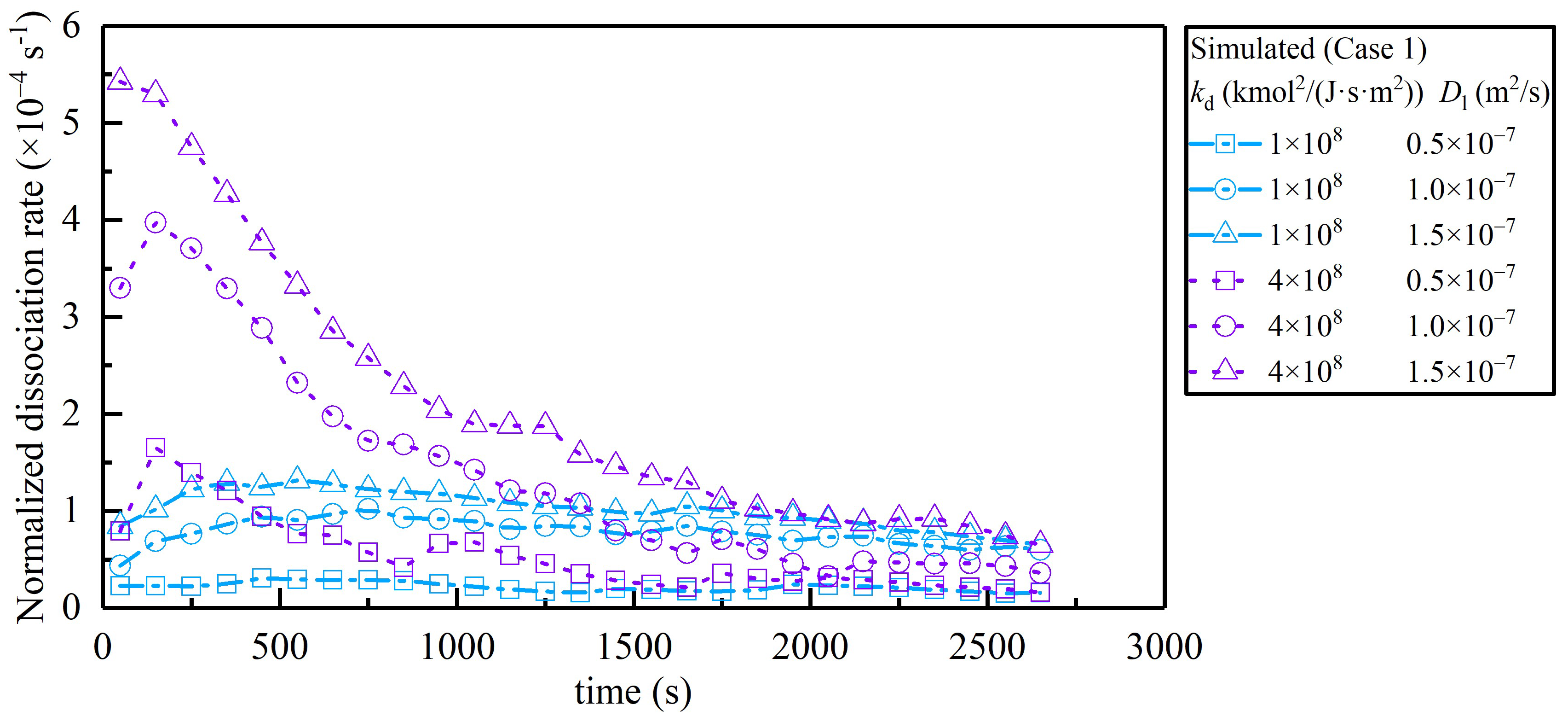
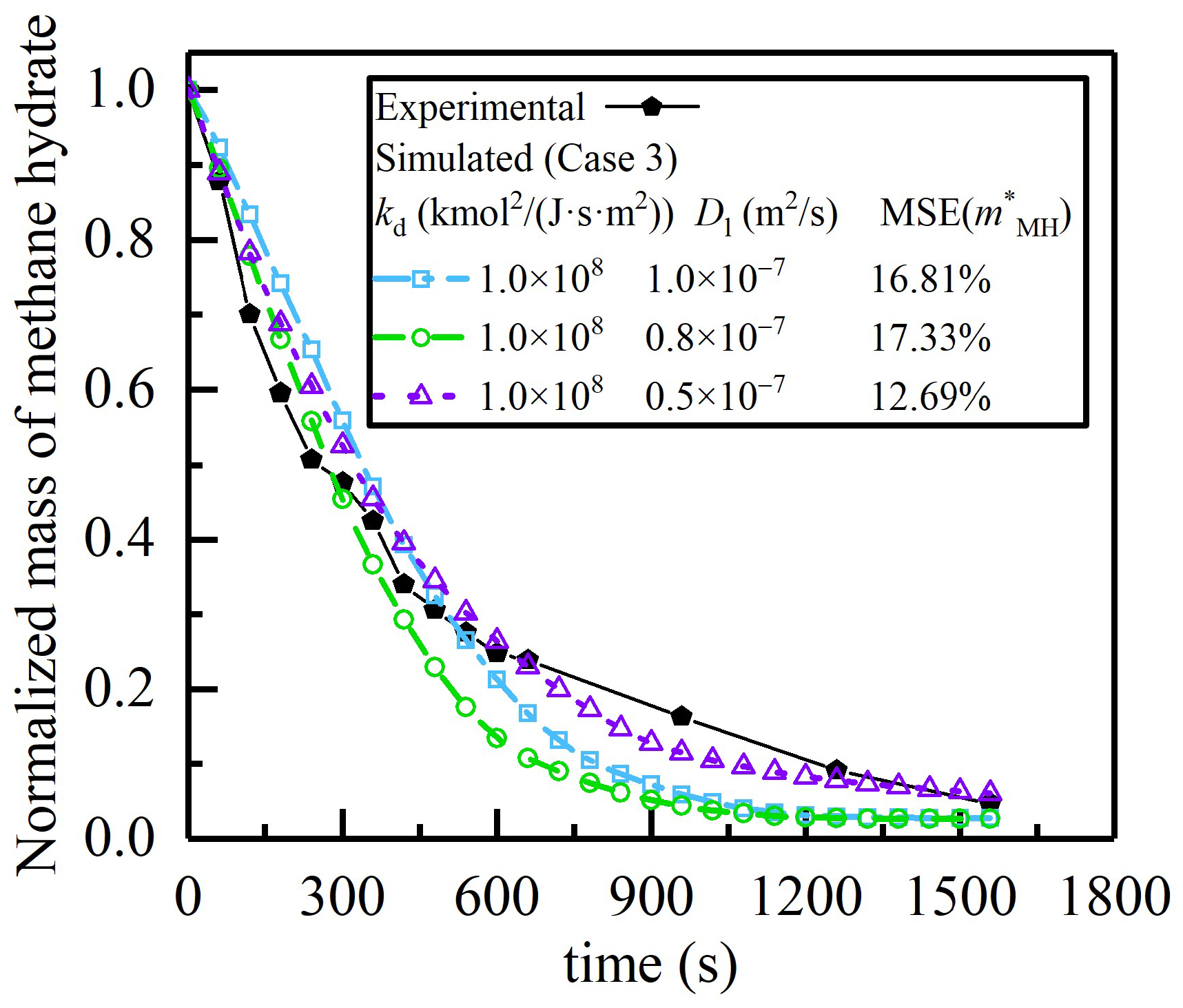
4.1. Estimation of Kinetic Parameters

As the rate constant is related to the system scale (e.g., pore scale, reactor scale, and field scale) and the dissociation conditions (e.g., temperature, pressure, and agitation), it is reliable to determine the rate constant from the experimental data. In addition, the formation of micro- and nanobubbles (MNBs) during hydrate dissociation in water was identified in previous studies, which accelerated the transport of dissolved methane to the gaseous phase. Considering the effect of MNBs, the equivalent diffusion coefficient of dissolved methane may be significantly improved by 1–2 orders of magnitude. Consequently, the value of the effective diffusion coefficient is difficult to specify, and data fitting is required to find a reasonable assignment. The normalized masses of methane hydrate from the experimental results and simulations of depressurization at small and large pressure differences were compared to determine the rate constant k_c0 and effective diffusion coefficient of methane in water D_l.

When evaluating the numerical results, the normalized mass of methane hydrate is determined as follows:

$$m^{*}{}_{\mathrm{MH}}(t)=\frac{{\displaystyle {\int }_V{\epsilon }_{\mathrm{MH}}(t)dV}}{{\displaystyle {\int }_V{\epsilon }_{\mathrm{MH}}dV}\left|{}_{t=0}\right.}$$

(18)

To quantify the agreement between experimental data and simulation results using different parameters, the mean square error (MSE) of the normalized mass from 300 s to 2700 s is calculated as follows:

$$\mathrm{MSE}(m^{*}{}_{\mathrm{MH}})=\sqrt{\frac{1}{N}{\displaystyle \sum _{i=1}^N{\left(\frac{m^{*}{}_{\mathrm{MH},\mathrm{sim}}-m^{*}{}_{\mathrm{MH},\exp }}{m^{*}{}_{\mathrm{MH},\exp }}\right)}_i{}^2}}$$

(19)

The normalized dissociation rate is also calculated based on the normalized mass at the adjacent time:

$$r^{*}{}_{\mathrm{MH}}\left(\frac{t_2+t_1}{2}\right)=\frac{m^{*}{}_{\mathrm{MH}}(t_2)-m^{*}{}_{\mathrm{MH}}(t_1)}{t_2-t_1}$$

(20)

Figure 5 shows the normalized mass evolution during hydrate dissociation under a small pressure difference (0.8 MPa). When the effective diffusion coefficient is D_l = 0.5 × 10⁻⁷ m²/s, the normalized mass deviates most significantly from experimental data, where the simulated dissociation rate is much smaller compared to the experimental rate, irrespective of the rate constant. However, when the effective diffusion coefficient is adjusted to D_l = 1.0 × 10⁻⁷ m²/s, and the rate constant is established at k_d = 2.0 × 10⁸ kmol²/(J·s·m²), the normalized mass aligns most closely with the experimental data, exhibiting a mean square error of 4.08%. Further variations are observed for cases employing an effective diffusion coefficient of 1.5 × 10⁻⁷ m²/s, as detailed in

Table 4. The mean square errors of the simulated normalized mass in case 1 compared to the experimental data.

Case Description	Case No.	kd (×108 kmol2/(J·s·m2))	Dl (×10−7 m2/s)	$\mathbf{MSE}({\dot{\mathit{m}}}^{*}{}_{\mathbf{MH}})$
Case 1: Hydrate dissociation with a pressure difference of 0.8 MPa	1a	1.0	0.5	30.22%
	1b	1.0	1.0	16.03%
	1c	1.0	1.5	9.50%
	1d	2.0	0.5	29.16%
	1e	2.0	1.0	4.08%
	1f	2.0	1.5	6.86%
	1g	4.0	0.5	20.37%
	1h	4.0	1.0	8.62%
	1i	4.0	1.5	26.31%
	1j	1.5	0.8	12.39%

.

Meanwhile, Figure 6 compares the variation in the dissociation rate with the effective diffusion coefficient for different rate constant values of 1.0 × 10⁸ kmol²/(J·s·m²) and 4.0 × 10⁸ kmol²/(J·s·m²), respectively. The dissociation rate rises as the rate constant increases from 1.0 × 10⁸ m/s to 4.0 × 10⁸ kmol²/(J·s·m²), particularly before t = 600 s. Additionally, with an equivalent rate constant, the time-averaged dissociation rate also increases with the effective diffusion coefficient. These quantitative findings suggest that the dissociation rate is influenced by both the kinetics and diffusion in the initial dissociation period. At a rate constant of 1.0 × 10⁸ kmol²/(J·s·m²), the dissociation rate displays minimal change over time. Conversely, the dissociation rate increases when the rate constant k_d = 4.0 × 10⁸ kmol²/(J·s·m²) decreases with time across all cases. This phenomenon is attributed to a substantial increase in the water layer thickness during rapid dissociation, leading to intensified diffusion resistance. It is noteworthy that, over time, the temporal dissociation rate tends to converge, regardless of the rate constant. Therefore, it implies that hydrate dissociation is predominantly governed by diffusion as the water layer thickens in the late stages of decomposition.

To ascertain the rate constant and effective diffusion coefficient with greater accuracy, the simulated distributions of residual methane hydrate at different times are compared with the experimental images. Figure 7 compares the hydrate dissociation under a small pressure difference. Experimental observations reveal a non-uniform initial hydrate thickness, with prominent methane hydrate preferentially dissociating within the initial 600 s. Subsequently, the dissociation front aligns essentially parallel to the gas–liquid interface, gradually progressing over the next 2100 s. This progression implies that methane diffusion in the water film begins to govern the dissociation rate. The hydrate evolution in Figure 7c,d shows consistent trends with the experiment images. Conversely, for an effective coefficient of 1.5 × 10⁻⁷ m²/s, the dissociation front in Figure 7e advances uniformly at all positions from the beginning, indicating that the dissociation is reaction-dominated. This simulation stands in contrast to the experimental results. Therefore, considering the comprehensive assessment encompassing the quantitative residual mass, dissociation rate, and visual evolution of the dissociation front, we deduce that the effective diffusion rate is approximately 1.0 × 10⁻⁷ m²/s in the simulation of case 1.

Furthermore, Figure 8 compares the concentration of methane dissolved along the direction of the water layer thickness for different values of the effective diffusion coefficient. The selection of simulation results at different time points ensures a consistent water layer thickness whenever possible. Observably, the hydrate at the dissociation front constitutes a porous region with an approximate thickness of 10 microns, wherein the volume fraction of the hydrate gradually transitions from 1 to 0. On the left of the dissociation front resides methane hydrate in the solid phase, exhibiting a methane concentration equivalent to the hypothetical equilibrium solubility of methane hydrate. With the increase in the effective diffusion coefficient, both the concentration gradient and the concentration proximate to the dissociation front diminish, thereby augmenting the driving force of hydrate dissociation. When the effective diffusion coefficient is fixed at D_l = 1.0 × 10⁻⁷ m²/s, the produced methane does not significantly increase in concentration near the dissociation front with the increasing reaction rate constant. Thus, the local concentration in the water layer near the dissociation front is mainly determined by the effective diffusion coefficient.

To comprehensively validate the applicability of the numerical model and associated parameters across varying dissociation rates, additional simulation cases were conducted based on experiments involving hydrate dissociation under a substantial pressure difference (2.84 MPa). Compared to case 1, the diffusion coefficient and rate constant that best agree with the experimental data are slightly different, as shown in Figure 9. Cases 2e (k_d = 1.0 × 10⁸ kmol²/(J·s·m²), D_l = 1.0 × 10⁻⁷ m²/s) and 2g (k_d = 2.0 × 10⁸ kmol²/(J·s·m²), D_l = 0.5 × 10⁻⁷ m²/s) are in good agreement with the experimental data, yielding mean square errors of 15.05% and 7.5%, respectively, as listed in

Table 5. The mean square errors of the simulated normalized mass in case 2 compared to the experimental data.

Case Description	Case No.	kd (×108 kmol2/(J·s·m2))	Dl (×10−7 m2/s)	$\mathbf{MSE}({\dot{\mathit{m}}}^{*}{}_{\mathbf{MH}})$
Case 2: Hydrate dissociation with pressure difference of 2.84 MPa	2a	0.5	0.5	103.54%
	2b	0.5	1.0	75.74%
	2c	0.5	1.5	50.97%
	2d	1.0	0.5	59.72%
	2e	1.0	1.0	15.05%
	2f	1.0	1.5	33.59%
	2g	2.0	0.5	7.50%
	2h	2.0	1.0	53.13%
	2i	2.0	1.5	67.01%
	2j	1.5	0.8	19.82%

. Several factors contribute to this variance: (1) the measurement uncertainty in temperature and pressure, which have a more pronounced impact on the experiment under a small pressure difference; (2) the distribution of hydrate along the thickness direction in the microfluidic chip, which cannot be observed in the experimental image; (3) the influence of the upper and lower wall surfaces of the microfluidic chip on hydrate dissociation, methane diffusion, and nucleation, which is not considered in the two-dimensional simulation.

Similar to case 1, hydrate dissociation under a large pressure difference is also diffusion-dominated. Figure 10 shows the initial loose distribution of methane hydrate in the pores, with dissociation initiating from particles near the gas–liquid interface. Notably, the left-side hydrate layer dissociates more rapidly than the right side due to the sparsity and thinness of hydrate in that region. As the water layer thickens, the dissociation rate gradually decelerates. The hydrate evolution in cases 2e (k_d = 1.0 × 10⁸ kmol²/(J·s·m²), D_l = 1.0 × 10⁻⁷ m²/s) and 2j (k_d = 1.5 × 10⁸ kmol²/(J·s·m²), D_l = 0.8 × 10⁻⁷ m²/s) is in the best agreement with the experimental images.

Combining the most consistent parameters in cases 1 and 2, we tested the simulations (cases 1j and 2j) with a rate constant of 1.5 × 10⁸ kmol²/(J·s·m²) and an effective diffusion coefficient of 0.8 × 10⁻⁷ m²/s. The mean square errors of cases 1j and 2j are 12.39% and 19.82%, respectively, which are acceptable compared to other parameters. By comprehensively comparing the simulated dissociation rate curves and hydrate evolution with the experimental data for different pressure differences, the rate constant and the effective diffusion coefficient are reliably determined to be k_d = 1.5 × 10⁸ kmol²/(J·s·m²) and D_l = 0.8 × 10⁻⁷ m²/s, respectively. The magnitude of the effective methane diffusion coefficient in water is close to Yang’s pore-scale numerical work based on the lattice Boltzmann method. The controlling mechanism of hydrate dissociation obtained in this paper also agrees with Yang’s work [10], which indicates that the intensified diffusion limitation with increased water saturation governed the hydrate dissociation rate.

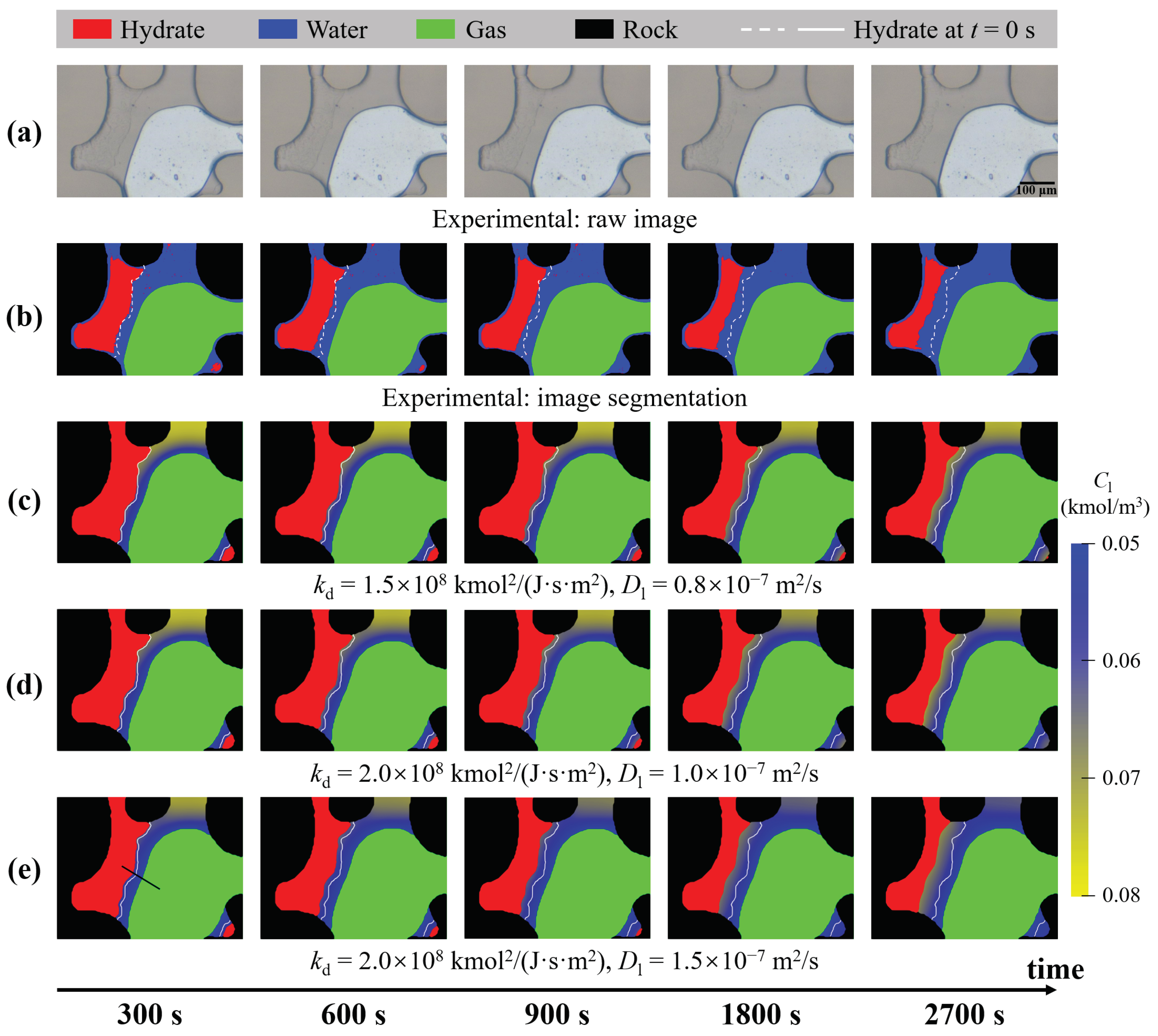
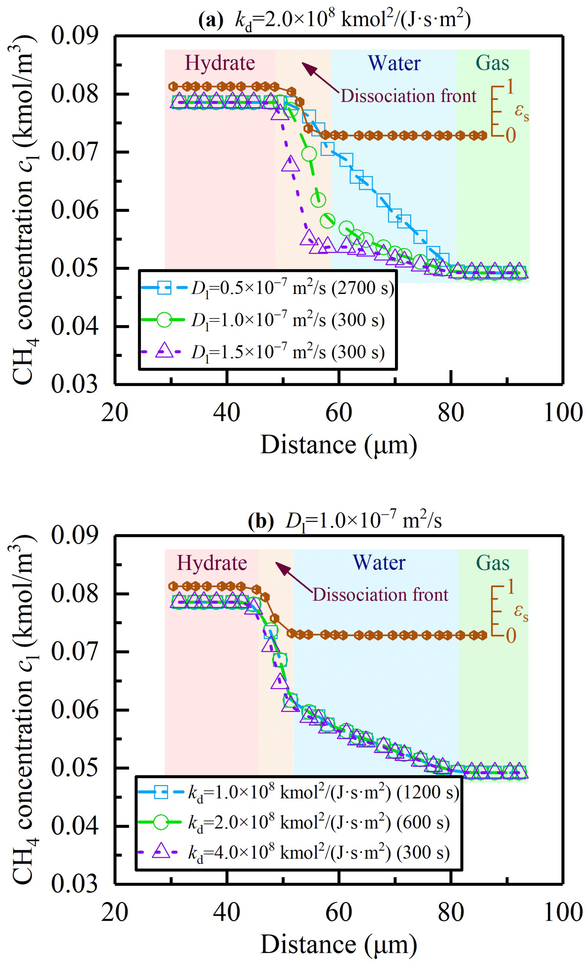
4.2. Verification of Unresolved Darcy-Scale Simulations

Loose hydrate particles usually contain sub-pore structures that are much smaller than the pores between sediment grains. If fine grids are used to characterize these sub-pores structures, the required grid number may be at least one order of magnitude higher than that of the sediment pores. To reduce computational resource consumption, it is feasible to replace the loose hydrate particles with a porous region with the porosity of their average volume fraction, as shown in Figure 11. The porosity and specific surface area of the porous region are calculated as follows:

$${\epsilon }_{\mathrm{p}}=\frac{{\displaystyle {\int }_V{\epsilon }_{\mathrm{MH}}dV}}{{\displaystyle {\int }_{V_{\mathrm{p}}}dV}}$$

(21)

$$A_{\mathrm{s},\mathrm{p}}=‖\nabla \left({\epsilon }_{\mathrm{p}}/{\epsilon }_{\mathrm{p},\mathrm{ini}}\right)‖$$

(22)

where $V$ and $V_{\mathrm{p}}$ represent the entire computational domain and the porous region, respectively, and ${\epsilon }_{\mathrm{p},\mathrm{ini}}$ represents the initial porosity of the porous region. Figure 12 and Figure 13 show that the dissociation rate and hydrate evolution with this method are in good agreement with the experimental data and simulations with the same diffusion coefficients and rate constants in case 2. The mean square errors are also similar to those of the fine structure in case 2. Thus, it is feasible to replace the complex structure of hydrate particles with a sub-grid porous region, which can effectively reduce the mesh size as the sediment pore is usually several times larger than that of hydrate particles.

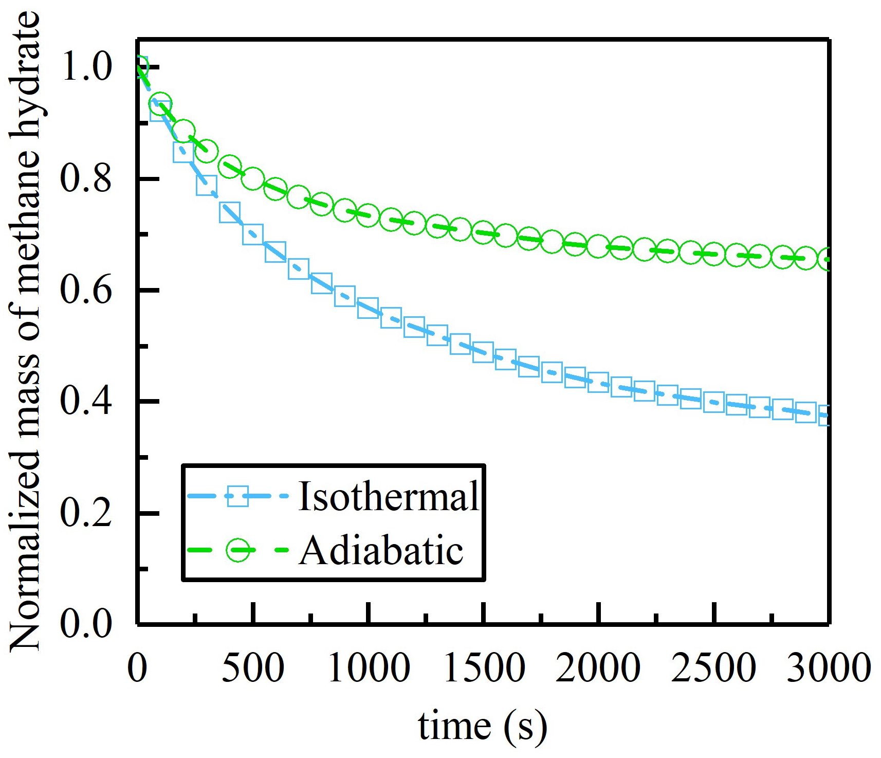
4.3. Effect of Temperature on Hydrate Dissociation

Among the existing microfluidic experiments on hydrate dissociation, the micromodel is usually immersed in a coolant, so depressurization-induced hydrate dissociation occurs in isothermal conditions. In contrast, hydrate dissociation at reactor and field scales is often accompanied by reservoir temperature changes. The heat required for dissociation is first supplied by the reservoir’s sensible heat and then by the ambient heat transfer. Due to the low thermal conductivity of the reservoir, the dissociation rate is fast at the beginning and gradually slows down as the temperature decreases. From the perspective of the pore scale, the initial stage of actual hydrate dissociation is more like adiabatic conditions than isothermal conditions. In this case, hydrate dissociation under isothermal and adiabatic conditions is compared to exhibit the difference between microfluidic experiments and actual exploitation conditions. The initial distribution of methane hydrate, water, and methane gas is shown in Figure 4a. The boundary conditions of the isothermal case are the same as those of case 1, while the adiabatic case changes the right boundary condition to a zero gradient. In order to avoid water freezing at a temperature below 0 °C, this case increases the equilibrium temperature and pressure of the methane hydrate phase. The hydrate equilibrium pressure is 7.2 MPa, and the dissociation pressure is 3 MPa. Figure 14 and Figure 15 show that heat absorbed by hydrate dissociation under adiabatic conditions decreases the reservoir temperature, which slows down the dissociation rate. In contrast, under isothermal conditions, the local temperature and the corresponding equilibrium pressure are constant, and thus, the dissociation rate is only affected by the concentration of methane in the liquid phase. Therefore, the rate of hydrate dissociation under adiabatic conditions is lower than that under isothermal conditions with increasing time. At 3000 s, the total mass of dissociated hydrate under adiabatic conditions is 55% of that under isothermal conditions, and the dissociation rate under adiabatic conditions is only 36% of that under isothermal conditions. The observed disparities in dissociation behavior can be attributed to the incorporation of heat transfer considerations, specifically the heat absorption linked to the endothermic dissociation process. This inclusion allows for the prediction of a continuous temperature decrease, concurrent with a shift in equilibrium conditions toward the lower-pressure zone. As the equilibrium pressure diminishes, hydrate dissociation tends to reach equilibrium more readily, resulting in earlier termination and a reduced yield of methane production, thereby influencing the overall dissociation dynamics. This is consistent with the trend of the hydrate dissociation rate with time in experiments at a large scale. Therefore, microfluidic experiments under isothermal conditions may overestimate the amount of dissociated hydrate and the dissociation rate during the depressurization process. Especially when the sensible heat is close to exhaustion, the dissociation rate under actual exploitation conditions may be at least one order of magnitude lower than that under isothermal conditions. However, the evolution of hydrate profiles under isothermal and adiabatic conditions shows similarities, as shown in Figure 16. At 100 s, the amount and distribution of residual hydrate are basically the same since the temperature drop under adiabatic conditions is not significant at this time. Although the dissociation rate is significantly reduced under adiabatic conditions, the hydrate distribution is close to that under isothermal conditions with the same amount of residual hydrate. Therefore, the hydrate evolution observed in microfluidic experiments is still useful for practical methane hydrate exploitation.

5. Conclusions

A multiscale numerical model based on the multiphase micro-continuum DBS framework was developed to simulate methane hydrate dissociation in porous media, including two-phase flow, heat and mass transfer, dissociation kinetics, and hydrate structure evolution. The proposed model was validated by microfluidic experiments. Experimental observations under different dissociation conditions were compared with a series of numerical simulations to determine the kinetic parameters of methane hydrate dissociation. By aligning the numerical and experimental results, the range of the rate constant and the effective diffusion coefficient are determined to be k_d = (1~2) × 10⁸ kmol²/(J·s·m²) and D_l = (0.5~1) × 10⁻⁷ m²/s, respectively. Both the experimental and simulated hydrate evolution results indicate that the diffusion of methane in the thick water film dominates the dissociation rate.

To reduce the computational demand, we propose conducting multiscale simulations based on a micro-continuum framework. Herein, the loose hydrate structure is treated as an effective porous medium, while the sediment pore is distinctly maintained as a pure fluid zone. The dissociation rate and hydrate evolution stemming from this methodology exhibit good agreement with experimental data and fine single-scale simulations utilizing equivalent diffusion coefficients and rate constants. These consistent simulations underscore the viability of conducting multiscale modeling for hydrate dissociation on massive grids, striking a balance between computational efficiency and accuracy.

To the best of our knowledge, few studies have been devoted to such calibration and validation between pore-scale simulations and experiments. Compared to the previous model, the calibrated pore-scale numerical model can provide a more confident capacity to simulate hydrate dissociation and thus offer more accurate insight into the underlying mechanism. Furthermore, comparisons between simulations of hydrate dissociation under isothermal and adiabatic conditions highlight distinctions between microfluidic experiments and practical exploitation scenarios. Specifically, under adiabatic conditions, the dissociation rate experiences a significant reduction. However, the distribution of hydrate closely resembles that under isothermal conditions with an equivalent residual hydrate quantity, underscoring the utility of microfluidic experiments in understanding certain dissociation dynamics.

In future work, the proposed multiscale micro-continuum model will be used to investigate the evolution and control mechanism of hydrate dissociation in multiscale porous media. Different hydrate occurrence modes and operating conditions, such as the driving force, hydrate pore habits, and the initial distribution of gas and water, will be considered in numerical research to better understand the multi-physical processes and mechanisms involved in hydrate dissociation.

References

1. Sloan, E.D. Gas hydrates: Review of physical/chemical properties. Energy Fuels 1998, 12, 191–196. [Google Scholar] [CrossRef]
2. Klauda, J.B.; Sandler, S.I. Global distribution of methane hydrate in ocean sediment. Energy Fuels 2005, 19, 459–470. [Google Scholar] [CrossRef]
3. Lee, S.-Y.; Holder, G.D. Methane hydrates potential as a future energy source. Fuel Process. Technol. 2001, 71, 181–186. [Google Scholar] [CrossRef]
4. Song, Y.; Yang, L.; Zhao, J.; Liu, W.; Yang, M.; Li, Y.; Liu, Y.; Li, Q. The status of natural gas hydrate research in China: A review. Renew. Sustain. Energy Rev. 2014, 31, 778–791. [Google Scholar] [CrossRef]
5. Hassanpouryouzband, A.; Joonaki, E.; Farahani, M.V.; Takeya, S.; Ruppel, C.; Yang, J.; English, N.J.; Schicks, J.M.; Edlmann, K.; Mehrabian, H. Gas hydrates in sustainable chemistry. Chem. Soc. Rev. 2020, 49, 5225–5309. [Google Scholar] [CrossRef]
6. Sloan Jr, E.D. Fundamental principles and applications of natural gas hydrates. Nature 2003, 426, 353–359. [Google Scholar] [CrossRef]
7. Pang, W.; Xu, W.; Sun, C.; Zhang, C.; Chen, G. Methane hydrate dissociation experiment in a middle-sized quiescent reactor using thermal method. Fuel 2009, 88, 497–503. [Google Scholar] [CrossRef]
8. Ji, C.; Ahmadi, G.; Smith, D.H. Natural gas production from hydrate decomposition by depressurization. Chem. Eng. Sci. 2001, 56, 5801–5814. [Google Scholar] [CrossRef]
9. Yuan, Q.; Sun, C.-Y.; Yang, X.; Ma, P.-C.; Ma, Z.-W.; Li, Q.-P.; Chen, G.-J. Gas production from methane-hydrate-bearing sands by ethylene glycol injection using a three-dimensional reactor. Energy Fuels 2011, 25, 3108–3115. [Google Scholar] [CrossRef]
10. Yang, J.; Dai, X.; Xu, Q.; Liu, Z.; Zan, C.; Long, W.; Shi, L. Pore-scale study of multicomponent multiphase heat and mass transfer mechanism during methane hydrate dissociation process. Chem. Eng. J. 2021, 423, 130206. [Google Scholar] [CrossRef]
11. Anderson, B.J.; Kurihara, M.; White, M.D.; Moridis, G.J.; Wilson, S.J.; Pooladi-Darvish, M.; Gaddipati, M.; Masuda, Y.; Collett, T.S.; Hunter, R.B. Regional long-term production modeling from a single well test, Mount Elbert gas hydrate stratigraphic test well, Alaska North slope. Mar. Pet. Geol. 2011, 28, 493–501. [Google Scholar] [CrossRef]
12. Farahani, M.V.; Guo, X.; Zhang, L.; Yang, M.; Hassanpouryouzband, A.; Zhao, J.; Yang, J.; Song, Y.; Tohidi, B. Effect of thermal formation/dissociation cycles on the kinetics of formation and pore-scale distribution of methane hydrates in porous media: A magnetic resonance imaging study. Sustain. Energy Fuels 2021, 5, 1567–1583. [Google Scholar] [CrossRef]
13. Li, X.-Y.; Li, X.-S.; Wang, Y.; Li, G.; Zhang, Y.; Hu, H.-Q.; Wan, K.; Zeng, H.-P. Influence of particle size on the heat and mass transfer characteristics of methane hydrate formation and decomposition in porous media. Energy Fuels 2021, 35, 2153–2164. [Google Scholar] [CrossRef]
14. Yin, Z.; Moridis, G.; Tan, H.K.; Linga, P. Numerical analysis of experimental studies of methane hydrate formation in a sandy porous medium. Appl. Energy 2018, 220, 681–704. [Google Scholar] [CrossRef]
15. Yu, M.; Li, W.; Jiang, L.; Wang, X.; Yang, M.; Song, Y. Numerical study of gas production from methane hydrate deposits by depressurization at 274 K. Appl. Energy 2018, 227, 28–37. [Google Scholar] [CrossRef]
16. Lei, L.; Seol, Y.; Jarvis, K. Pore-scale visualization of methane hydrate-bearing sediments with micro-CT. Geophys. Res. Lett. 2018, 45, 5417–5426. [Google Scholar] [CrossRef]
17. He, G.; Luo, X.; Zhang, H.; Bi, J. Pore-scale identification of multi-phase spatial distribution of hydrate bearing sediment. J. Geophys. Eng. 2018, 15, 2310–2317. [Google Scholar] [CrossRef]
18. Tohidi, B.; Anderson, R.; Clennell, M.B.; Burgass, R.W.; Biderkab, A.B. Visual observation of gas-hydrate formation and dissociation in synthetic porous media by means of glass micromodels. Geology 2001, 29, 867–870. [Google Scholar] [CrossRef]
19. Katsuki, D.; Ohmura, R.; Ebinuma, T.; Narita, H. Methane hydrate crystal growth in a porous medium filled with methane-saturated liquid water. Philos. Mag. 2007, 87, 1057–1069. [Google Scholar] [CrossRef]
20. Almenningen, S.; Flatlandsmo, J.; Fernø, M.A.; Ersland, G. Multiscale laboratory verification of depressurization for production of sedimentary methane hydrates. SPE J. 2017, 22, 138–147. [Google Scholar] [CrossRef]
21. Farahani, M.V.; Hassanpouryouzband, A.; Yang, J.; Tohidi, B. Development of a coupled geophysical–geothermal scheme for quantification of hydrates in gas hydrate-bearing permafrost sediments. PCCP 2021, 23, 24249–24264. [Google Scholar] [CrossRef] [PubMed]
22. Jeong, S.-M.; Hsieh, L.-H.C.; Huang, C.-Y.; Sean, W.-Y. Direct numerical simulation of CO2 hydrate dissociation in pore-scale flow by applying CFD method. Int. J. Heat Mass Transf. 2017, 107, 300–306. [Google Scholar] [CrossRef]
23. Mohammadmoradi, P.; Kantzas, A. Direct geometrical simulation of pore space evolution through hydrate dissociation in methane hydrate reservoirs. Mar. Pet. Geol. 2018, 89, 786–798. [Google Scholar] [CrossRef]
24. Zhang, L.; Zhang, C.; Zhang, K.; Zhang, L.; Yao, J.; Sun, H.; Yang, Y. Pore-scale investigation of methane hydrate dissociation using the lattice Boltzmann method. Water Resour. Res. 2019, 55, 8422–8444. [Google Scholar] [CrossRef]
25. Wang, X.; Dong, B.; Chen, C.; Li, W.; Song, Y. Pore-scale investigation on the influences of mass-transfer-limitation on methane hydrate dissociation using depressurization. Int. J. Heat Mass Transf. 2019, 144, 118656. [Google Scholar] [CrossRef]
26. Wang, X.; Dong, B.; Wang, F.; Li, W.; Song, Y. Pore-scale investigations on the effects of ice formation/melting on methane hydrate dissociation using depressurization. Int. J. Heat Mass Transf. 2019, 131, 737–749. [Google Scholar] [CrossRef]
27. Yang, J.; Xu, Q.; Liu, Z.; Shi, L. Pore-scale study of the multiphase methane hydrate dissociation dynamics and mechanisms in the sediment. Chem. Eng. J. 2022, 430, 132786. [Google Scholar] [CrossRef]
28. Soulaine, C.; Roman, S.; Kovscek, A.; Tchelepi, H.A. Mineral dissolution and wormholing from a pore-scale perspective. J. Fluid Mech. 2017, 827, 457–483. [Google Scholar] [CrossRef]
29. Scheibe, T.D.; Perkins, W.A.; Richmond, M.C.; McKinley, M.I.; Romero-Gomez, P.D.; Oostrom, M.; Wietsma, T.W.; Serkowski, J.A.; Zachara, J.M. Pore-scale and multiscale numerical simulation of flow and transport in a laboratory-scale column. Water Resour. Res. 2015, 51, 1023–1035. [Google Scholar] [CrossRef]
30. Xu, Q.; Dai, X.; Yang, J.; Liu, Z.; Shi, L. Image-based modelling of coke combustion in a multiscale porous medium using a micro-continuum framework. J. Fluid Mech. 2022, 932, A51. [Google Scholar] [CrossRef]
31. Yang, F.; Stack, A.G.; Starchenko, V. Micro-continuum approach for mineral precipitation. Sci. Rep. 2021, 11, 3495. [Google Scholar] [CrossRef] [PubMed]
32. Horgue, P.; Prat, M.; Quintard, M. A penalization technique applied to the “Volume-Of-Fluid” method: Wettability condition on immersed boundaries. Comput. Fluids 2014, 100, 255–266. [Google Scholar] [CrossRef]
33. Soulaine, C.; Roman, S.; Kovscek, A.; Tchelepi, H.A. Pore-scale modelling of multiphase reactive flow: Application to mineral dissolution with production of. J. Fluid Mech. 2018, 855, 616–645. [Google Scholar] [CrossRef]
34. Carrillo, F.J.; Bourg, I.C.; Soulaine, C. Multiphase flow modeling in multiscale porous media: An open-source micro-continuum approach. J. Comput. Phys. X 2020, 8, 100073. [Google Scholar] [CrossRef]
35. Liu, Z.; Yang, J.; Xu, Q.; Shi, L. Improved micro-continuum approach for capillary-dominated multiphase flow with reduced spurious velocity. Phys. Fluids 2022, 34, 122108. [Google Scholar] [CrossRef]
36. Sean, W.Y.; Sato, T.; Yamasaki, A.; Kiyono, F. CFD and experimental study on methane hydrate dissociation. Part II. General cases. AlChE J. 2007, 53, 2148–2160. [Google Scholar] [CrossRef]
37. Maes, J.; Menke, H.P. GeoChemFoam: Direct modelling of multiphase reactive transport in real pore geometries with equilibrium reactions. Transp. Porous Media 2021, 139, 271–299. [Google Scholar] [CrossRef]
38. Jasak, H.; Jemcov, A.; Tukovic, Z. OpenFOAM: A C++ library for complex physics simulations. In Proceedings of the International Workshop on Coupled Methods in Numerical Dynamics, Dubrovnik, Croatia, 19–21 September 2007; pp. 1–20. [Google Scholar]
39. Van Leer, B. Towards the ultimate conservative difference scheme. J. Comput. Phys. 1997, 135, 229–248. [Google Scholar] [CrossRef]
40. Maes, J.; Soulaine, C. A unified single-field Volume-of-Fluid-based formulation for multi-component interfacial transfer with local volume changes. J. Comput. Phys. 2020, 402, 109024. [Google Scholar] [CrossRef]
41. Issa, R.I. Solution of the implicitly discretised fluid flow equations by operator-splitting. J. Comput. Phys. 1986, 62, 40–65. [Google Scholar] [CrossRef]
42. Maes, J. GeoChemFoam User Guide. Available online: https://github.com/GeoChemFoam/GeoChemFoam/blob/main/GeoChemFoam-User-Guide.pdf (accessed on 9 March 2022).
43. Yang, J. Pore-scale Visualization of Hydrate Dissociation and Mass Transfer during Depressurization Using Microfluidic Experiments. Fuel, 2023; in press. [Google Scholar]
44. Brooks, R.H. Hydraulic Properties of Porous Media; Colorado State University: Fort Collins, CO, USA, 1965. [Google Scholar]
45. Van Genuchten, M.T. A closed-form equation for predicting the hydraulic conductivity of unsaturated soils. Soil Sci. Soc. Am. J. 1980, 44, 892–898. [Google Scholar] [CrossRef]
46. Xu, Q.; Long, W.; Jiang, H.; Ma, B.; Zan, C.; Ma, D.; Shi, L. Quantification of the microstructure, effective hydraulic radius and effective transport properties changed by the coke deposition during the crude oil in-situ combustion. Chem. Eng. J. 2018, 331, 856–869. [Google Scholar] [CrossRef]
47. Haroun, Y.; Legendre, D.; Raynal, L. Volume of fluid method for interfacial reactive mass transfer: Application to stable liquid film. Chem. Eng. Sci. 2010, 65, 2896–2909. [Google Scholar] [CrossRef]
48. Maes, J.; Soulaine, C. A new compressive scheme to simulate species transfer across fluid interfaces using the volume-of-fluid method. Chem. Eng. Sci. 2018, 190, 405–418. [Google Scholar] [CrossRef]
Figure 1. Schematic of the resolved pore scale (macropores) and the unresolved Darcy scale (micropores).
Energies 16 07599 g001
Figure 2. Flow chart of the numerical model.
Energies 16 07599 g002
Figure 3. Schematics of the experimental apparatus.
Energies 16 07599 g003
Figure 4. Schematics of the initial computation domain of (a) case 1 and (b) case 2.
Energies 16 07599 g004
Figure 5. Normalized mass of methane hydrate dissociation under a small pressure difference (0.8 MPa).
Energies 16 07599 g005
Figure 6. Normalized dissociation rate under a small pressure difference (0.8 MPa).
Energies 16 07599 g006
Figure 7. Comparison of experimental and simulated hydrate evolution in case 1, (a) raw experimental image, (b) segmented experimental image, and (ce) simulation results of different rate constant and effective diffusion coefficient.
Energies 16 07599 g007
Figure 8. Simulated concentration profile along the solid black line in Figure 7e for (a) different diffusion coefficients and (b) different rate constants.
Energies 16 07599 g008
Figure 9. Normalized mass during hydrate dissociation under a large pressure difference (2.84 MPa).
Energies 16 07599 g009
Figure 10. Comparison of experimental and simulated hydrate evolution in case 2, (a) raw experimental image, (b) segmented experimental image, and (ce) simulation results of different rate constant and effective diffusion coefficient.
Energies 16 07599 g010
Figure 11. Schematic of using a porous region to replace loose hydrate particles.
Energies 16 07599 g011
Figure 12. Normalized mass during hydrate dissociation in case 3.
Energies 16 07599 g012
Figure 13. Comparison of experimental and simulated hydrate evolution in case 3, (a) raw experimental image, (b) segmented experimental image, and (ce) simulation results of different rate constant and effective diffusion coefficient.
Energies 16 07599 g013
Figure 14. Temperature variation with time in simulations under isothermal and adiabatic conditions.
Energies 16 07599 g014
Figure 15. Normalized mass during hydrate dissociation under isothermal and adiabatic conditions.
Energies 16 07599 g015
Figure 16. Comparison of hydrate evolution under (a) isothermal condition, and (b) adiabatic condition.
Energies 16 07599 g016