

Fast Power System Transient Stability Simulation

1
Institute of Technology, School of Electrical and Computer Engineering (SECE), Hawassa University, Hawassa, Ethiopia
2
Institutes of Electrical Power Systems, University of Duisburg-Essen, 47057 Duisburg, Germany
*
Authors to whom correspondence should be addressed.
Energies 2023, 16(20), 7157; https://doi.org/10.3390/en16207157
Submission received: 24 August 2023
/
Revised: 10 October 2023
/
Accepted: 16 October 2023
/
Published: 19 October 2023
(This article belongs to the Topic Energy Systems Planning, Operation and Optimization in Net-Zero Emissions)
Abstract
:Power system transient stability simulation is of critical importance for utilities to assess dynamic security. Most of the commercially available tools use the traditional numerical integration method to simulate power system transient stability, which is computationally intensive and has low simulation speed. This makes it difficult to identify any insecure contingency before it happens. It is already proven that power system transient stability simulation achieved using the differential transformation method (DTM) requires less computational effort and has improved simulation speed, but it still requires further improvement regarding its accuracy and performance efficiency. This paper introduces a novel power system transient stability simulation method based on the adaptive step-size differential transformation method. Using the proposed method, the step size is varied based on the estimated local solution error at each time step. The accuracy and speed of the proposed simulation approach are investigated in comparison with the classical differential transformation method and the traditional numerical integration method using the IEEE 9 bus and 39 bus test systems. The simulation results reveal that the proposed method increases the simulation speed by 20–44.57% and 83–92% when compared with the classical DTM and traditional numerical-integration-based simulation methods, respectively. It is also proved that compared with the DTM-based simulation, the proposed method provides 45.27% to 58.85% and more than 90% accurate simulation results for IEEE 9 and IEEE 39 test systems, respectively. Therefore the proposed power system transient stability simulation method is faster and relatively more accurate and can be applied for online transient stability monitoring of power system networks.
1. Introduction
Modern society is very dependent on the availability of electric energy; therefore, reliable electricity supply is foundational to all economic and societal activities. To supply this continuously growing demand, the size and complexity of the power supply systems with stochastic generation (due to renewable energy systems) is increasing. This pushes power systems to operate more and more closely to stability limits [1]. The increase in the share of renewable energy system (RES) generations further results in the increased problem of reduced system inertia, which brings power systems to conditions of lower reliability, safety, and stability. This implies that stability, specifically transient stability, plays a significant role as an index of robustness of power systems, subject by its nature to faults and disturbances [2,3].
Transient stability is the ability of the power system after exposure to large disturbance to transit to a stable state [4]. Transient stability analysis investigates the dynamic behavior of a power system for several seconds following a large disturbance. Inability to detect system instability behavior in a sufficient time interval to launch the corrective actions could result in a system failure at one location on a system that can quickly degenerate to cascading failures, which is usually the mechanism for large collapses or blackout of the system. Fast and accurate assessment of transient stability is of great significance for safe and stable operation of power systems.
To identify any unstable system condition before it happens, transient stability assessment is expected to be transitioned from offline or day-ahead studies to the online operation environment. Traditional methods of transient stability simulation rely on numerical integration, such as the Runge–Kutta or Euler techniques, to solve the differential algebraic equations governing power system dynamic behaviors. These solution methods, including implicit and explicit methods, are commonly used in commercial software packages with small enough integration steps of typically one to a few milliseconds to meet accuracy requirements [5]. However, these methods are computationally intensive, especially in large-scale systems with numerous contingencies. The power industry and the research community are seeking next-generation tools that are more powerful for power system online transient stability simulation.
Several previous works have been explored different aspects of transient stability analysis and simulation. For instance, ref. [6,7,8] used a coherency-based model reduction approach that aggregates a group of coherent generators in an equivalent generator, in which both the differential and algebraic equation models are simplified or reduced. Furthermore, to avoid solving nonlinear algebraic network equations separately from solving differential equations, many transient stability analysis and simulation tools assume all constant impedance loads and drive an ordinary differential equation model [6]. Such methods can result in substantial assessment and simulation errors. The parareal in time method by [9] involves parallel computers by decomposing a power system differential algebraic model or computation tasks to multiple processors to reduce simulation time. Similarly, the domain and multidecomposition methods by [10,11] involve parallel-computers-based computation tasks. But, still, the computation tasks are based on the traditional numerical algorithm to solve power system differential algebraic equations that require small enough integration steps and numerical iterations.
The semianalytical method proposed by [12,13,14] shifts some of the computation burdens from the online stage to the offline stage. In these methods, the offline drive approximates analytical solutions of differential equations for the purpose of online simulation. However, the network equations with power system differential algebraic model equations are still solved by traditional numerical iterations. The other semianalytical method proposed by [15,16], designed a differential transformation method (DTM)-based high-order semianalytical-based power system transient stability simulation scheme that allows significantly prolonged time steps to reduce simulation time compared to a traditional numerical approach. But this method assumes all loads as constant impedance so as to eliminate the network equations of a power system differential algebraic model and drive an ordinary differential equation model.
A variable time-step-based power system transient stability simulation was proposed by [17,18]. The integration time step control is performed based on the system behavior during the course of simulation. The method uses small time steps when the system variables are changing rapidly and large time steps when the system variables do not exhibit rapid variations. Solution error is estimated and the time step is adjusted to meet the specified tolerance threshold at each iteration step. This reduces the number of iterations and can also be used with more complex integration schemes. However, (1) at each iteration step, if the estimated solution error is greater than the specified tolerance threshold, the current solution is rejected and the solution procedures are repeated again using the new step size, which increases simulation time cost. (2) Still, algebraic equations are solved by iteration after each integration steps; this also has an impact on total simulation time cost.
An adaptive time step approach to dynamical simulation based on monitoring the conservation of energy was proposed by [19]. The method considers a physical object’s velocity and positions error estimate to determine the next time step. Using this method, numerical stability and computational efficiency (speed) were improved when compared with the traditional fixed-step numerical integration method. However, the method is independent of the system model equations describing its dynamic behaviors.
A differential transformation method (DTM)-based simulation algorithm proposed by [20], is fully analytical method. This method approximates the solution of complex power system differential algebraic model equations as a truncated power series of time. The approach is flexible in handling power system with any model detail without limitations. It also requires less computation effort and simulation time cost. However, differential transformation method gives a good approximation to the true solution in a very small region. To extend the region of solution convergence and improve accuracy of the results, DTM is applied at equal and fixed time interval as proposed by [21,22,23,24], up to the end of simulation period. In some cases, a very small sub division of interval is required with this method, which results in more computational effort and increased simulation time cost.
In this paper, an adaptive step size differential transformation method (AsDTM)-based power system transient stability simulation algorithm is proposed. This work introduces a novel step-size control algorithm based on local convergence error results at the end of each simulation time step by using the differential transformation method (DTM). The proposed novel power system transient stability simulation algorithm (1) is relatively robust and accurate, because it is flexible in handling power systems with any model detail and complexity without limitations; (2) improves simulation speed and accuracy based on control of local convergence error at each time step; (3) local solution error is estimated from only the last coefficient terms of the state and algebraic variables without any further calculations as in the variable step-size algorithm using traditional numerical integration methods; and (4) the solution obtained for the current simulation time step can be used during the next simulation time step without any limitations, such that the number of steps required to complete the transient stability simulation process reduces. These enable the proposed simulation scheme to be applied as an online transient stability simulation tool in small and medium-sized power systems.
The rest of the paper is organized as follows: Section 2 presents a description of the proposed method of power system transient stability simulation, Section 3 presents comparative analysis based on simulation results from the proposed method, traditional numerical integration method, and the classical DTM method, using IEEE test systems, and Section 4 presents conclusions and future work.
2. The Proposed Power System Transient Stability Simulation
2.1. Differential Transformation Method (DTM)
The differential transformation method (DTM) is a new emerging mathematical tool in power system analysis and simulation. The theory of the differential transformation method was originally established in [25] to derive approximate solutions of nonlinear differential equations and is defined below. Next, it was developed by researchers in the fields of mathematics and physics to obtain semianalytical solutions of various nonlinear dynamic systems. In [15,16,20,21,22,23,24,25], this method was examined for real-life complex network systems like power systems modeled by high-order nonlinear differential equations. DTM is defined as follows:
Definition: Consider a function x(t) of a real continuous variable t. The differential transformation (DT) of x(t) is defined by Equation (1), and the inverse DT of X(k) is defined by Equation (2), where k represents the order differential transformation (DT) [13,14,15].
The DT method provides various transformation rules for numerous generic functions [13,14,15,16,17,18], for both linear and nonlinear functions and for both simple and compositional functions, such that a differential equation in a continuous set about the variable t (time) is converted to a new set of difference equations in a discrete set about the variable k (the power series order) [25].
In power system simulation, DTM can be used as an explicit, fast, and robust solver of power system complex differential algebraic equations (DAEs). It is proved that the performance efficiency of a DTM is much better than that of the traditional numerical integration methods, because when using the DTM method, the iteration to solve algebraic equations after each integration step is eliminated and has a higher radius of convergence. To solve multimachine power system DAE models using the DTM method, the process is as follows: (1) transform power system DAE equations, (2) calculate the coefficients of state and algebraic variables, and (3) perform inverse transformation to determine state and algebraic variables as a function of time. Details of these procedures are presented in the following subsections.
2.2. Stability and Convergence Properties of the Proposed Method
In this paper, differential transformation method (DTM)-based fast power system transient stability simulation is introduced. In this subsection, the stability and convergence properties of the proposed method are demonstrated using the initial value problem.
Consider the following initial value problem, Equation (3), where and :
where y = (y1, y2, … yn) and the interval [0, T] is partitioned into N subdomains with grid points expressed as t0, t1, …, tj−1, tj = T, such that tj+1 = tj + h. Using the DTM solution approach, the first step is to determine the DTs of Equation (3), which is given as Equation (4) below, where K is the order of DT and m is the number of variables:
By eliminating 1/k from the right side of Equation (4), we can rewrite it as Equation (5), where Ymn and F are the transformed vector valued functions:
As we can see from Equation (5) above, the coefficient terms Ym,n(k) can be explicitly determined from the lower-order coefficients terms recursively.
After all the coefficient terms from k = 0 up to k = K are known, the exact solution of Equation (3) at a point t = tn+1 = tn + h can be written in the form of Taylor expansion, considering m number of variables, as Equation (6), where h represents the step size:
where ξn is a local truncation error and n = 0, 1, 2, … N − 1. The local truncation error can be expressed in the form of residual formula of Taylor series, considering m number of vectors of variable Yn, and is expressed as Equation (7):
This shows that the method approximates locally to the exact solution with order k. In this paper, the step size h is varied based on imposing the maximum of absolute value of the last coefficient terms to be lower than the admissible local error. This can be obtained by replacing ξn in Equation (7) by the admissible local error . Therefore, the new step size is calculated from Equation (8), where is the admissible local truncation error:
To check the convergence properties of the proposed method, we need to have a bounded global error and thus know stability requirements of the method. Let us consider a linear system equation, Equation (9):
And let for n = 0, 1, 2,…, N. The DTM method for this equation yields the following discretization:
The DT of Equation (9) is given by Equation (11) by eliminating 1/k:
where F(k) is DTs of C(t). With the recursive relation (11) the general term Ym,n(k) can be stated as Equation (12):
Subtracting Equation (10) from Equation (6) and using the general term (12) yields Equation (13):
where δn = hξn and .
Note that the method is said to be consistent of order p if ‖δn‖ = O(hp+1). To relate global discretization error with the initial error ξ0 and local discretization error, recursive relation (14) becomes Equation (15):
Here, the stability of the method depends on the bound of the term for all (tn + h) ≤ T. Therefore, considering the stability criterion ≤ S (stability constant), for all n ≥ 0 and (tn + h) ≤ T, the error norm bound is
Then, using the definition of local discretization error for all p and
, and also assuming y(0) = y0, leads to the following error norm inequality:
for all n = 0, 1, 2, … N. Thus, whenever the exact solution is smooth and the stability criterion given above is satisfied, the proposed method converges to the exact solution.
2.3. Description of the Proposed Method
Power system transient stability simulation is one of the most critical functions of an online dynamic security assessment (DSA). Traditional numerical integration method is commonly used in commercially available power system transient stability simulation tools. Speed of computation remains the most critical challenge for its application in an online transient stability simulation. It was proved that the DTM-based transient stability simulation method reduces the impact of computation burden. For online application, the DTM-based simulation method still requires further improvement regarding its accuracy and performance efficiency. This paper focuses on developing a new and novel power system transient stability simulation algorithm that significantly improves simulation efficiency and accuracy.
For practical implementation of numerical methods of solving differential algebraic equations, the use of variable step-size length is a crucial issue because it allows us to automate the control of error. The proposed simulation method solves complex power system DAE models using the differential transformation method at variable time steps. The step size is varied based on the local truncation error control algorithm, as in Equation (8). The automatic controls of step-size length are performed based on the following principles:
- Reduce the time step length when the error is above the tolerable error limit, to improve the accuracy of simulation.
- Increase the time step length when the error is below the tolerable error limit, to avoid unnecessary computational burden and improve the overall efficiency.
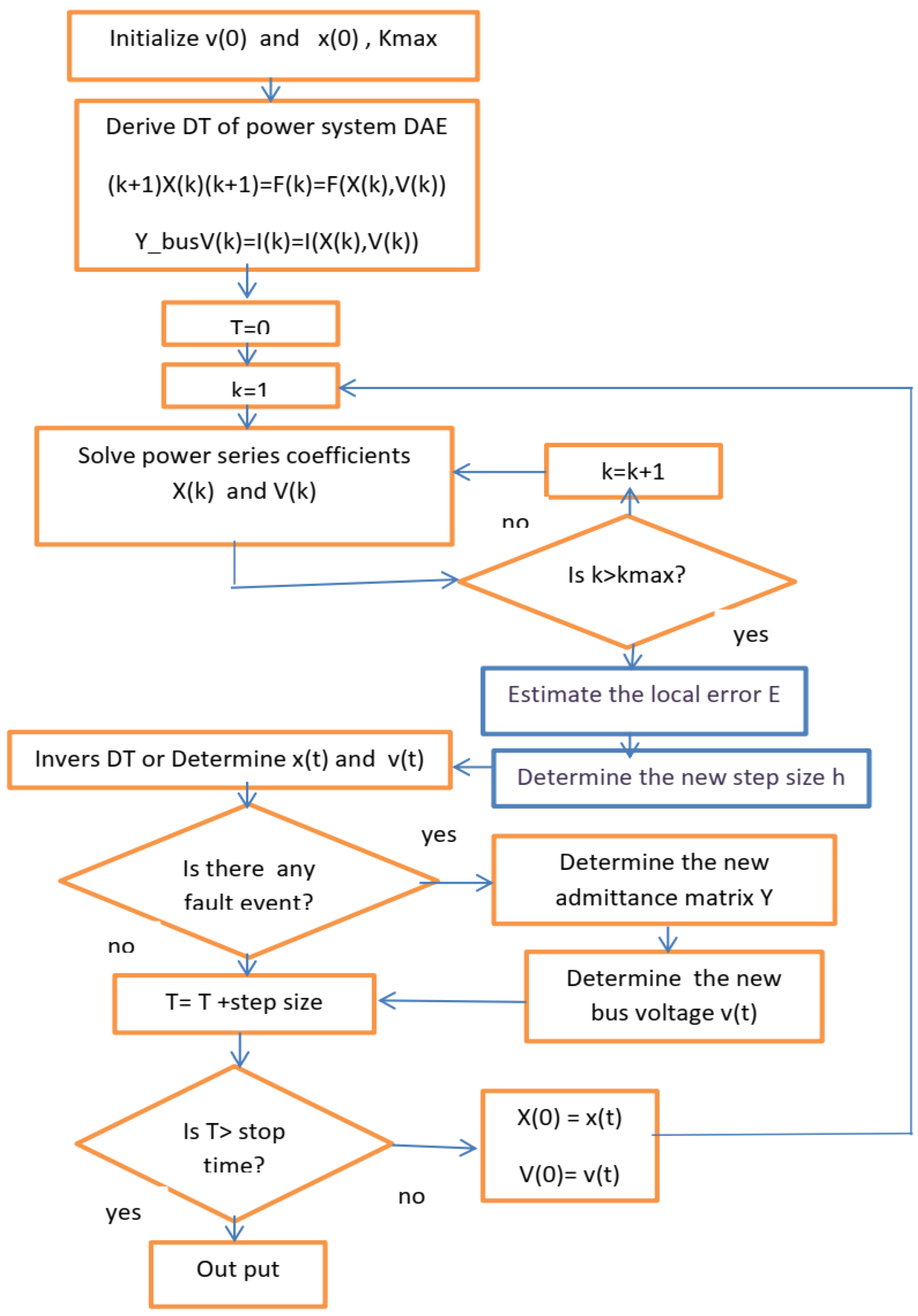
Figure 1 shows a flowchart of the proposed AsDTM-based transient stability simulation algorithm. In this subsection, each block of the proposed method of power system transient stability simulation will be described in more detail as follows:
Consider a power system with n bus and m machine DAE models in which generators are represented by a two-axis fourth-order model, all with a Type_1 excitation and voltage regulation system, as well as turbine/governor models, and all system loads are represented by constant impedance loads with both the network and stator algebraic equations represented by real matrices (expressed in rectangular form).
Consider also the state space representation of the power system DAE model equations as given by Equation (18), where x is the state vector, v is the vector of bus voltages, f represents a vector field determined by differential equations on dynamic devices such as synchronous generators and associated controllers, i is the vector valued function on current injections from all generators and load buses, and Ybus is the network admittance matrix.
where x(t) represents
and j = 1, 2, 3 … m, represent machine number.
Step 1. Derive DTs of power system DAEs:
Apply the differential transformation to functions given by Equation (18) on both sides, by using transformation to obtain Equation (19):
where X represents .
The vector valued function in Equation (17) represents both generators and load current injections. But here, for this specific case, constant impedance loads are considered and are included in the network admittance matrix Ybus. The differential transformation of the stator algebraic equation, Equation (20), can be derived and represented by Equation (22).
Let , and the generator current injection equation is
Differential transformations of r, , and are given as
where .
Therefore, the differential transformation of the generator current injection equation is
The load current injection at each bus is represented by
Finally, DTs of the network algebraic equation are given as Equation (24):
where .
Step 2. Solve power series coefficients:
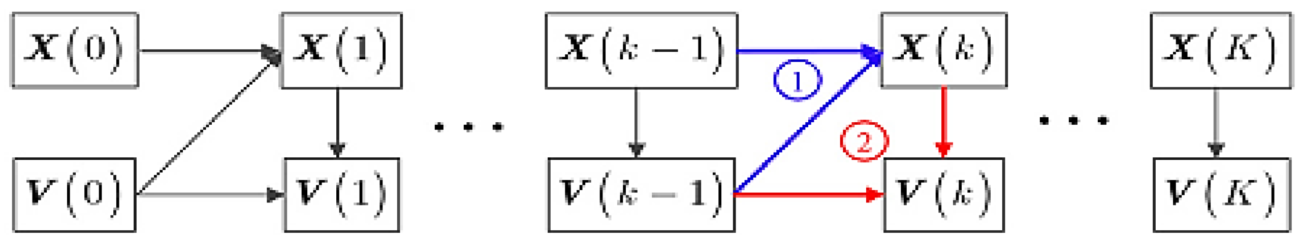
This step is initialized by the initial values of bus voltage V(0) and state variables X(0). The main task here is to solve power series coefficients X(k) and V(k) from the (k − 1)th-order coefficients, as indicated by the two circled numbers in Figure 2. Thus, any order coefficients are solvable from X(0),V(0).
The coefficients of state variables X(k) for differential equations are derived from Equation (19a) recursively from X(1) up to X (k), as shown in Figure 2. But when solving the coefficients of algebraic variables, bus voltage V(k) is not straightforward since V(k) appears on both sides, as we can observe from Equation (19b). If ZIP load models are considered the current injunction equations for constant power, and constant current load portions of the ZIP load are nonlinear and will be turned into linear in terms of their coefficients, the proof is given by [20]. Since constant impedance load is considered in this paper, the DT of the generator current injection equation given by Equation (22) can be rewritten as Equation (25) below.
And let
Since the load current injection is zero, letting represent zeros (2,2), represent zeros (2,1) at each of the n buses, for machine buses, and at (n − m) buses, then represents (2 × n) by (2 × n) matrixes and B represents (2 × n) by 1 column vector. Therefore, the current injections into the network from all the buses can be
where .
The detailed derivation of matrix A and B for other types of load model is not the focus of this paper but it is available in [20]. Considering constant impedance loads, the coefficients of bus voltages V(k) for all the network buses and coefficients of state variables X(k) are solved from Equation (29) from a–c recursively from X(1) up to X(k) and V(1) up to V (k).
Step 3. Determine the new step size (hnew):
As described in the previous subsections, the proposed simulation method solves complex power system DAE models using the differential transformation method at variable time steps. The step size is varied based on the local truncation error control algorithm, as in Equation (8). The main term of this local truncation error is known in the form of |Y(k)|tk (see Equation (8) [22]), where t is the local time variable in subinterval [tm, tm+1] and m is the number of subintervals between [0,T]. In this paper, the series term |Y(k)|tk is used as a local truncation error estimate of the power series of degree k. Therefore, without any further calculation, we can estimate the simulation step size that ensures the prescribed local admissible error by using just one of the coefficient terms [22,23]. The equation to calculate the step size (h) given by Equation (8) above is adopted and applied for power system transient stability simulation, as described below.
Let Mst, EXst, and TGst be matrix of generators, exciters, and turbine governor state variable, respectively. If m and N represent the number of machines and state variables, respectively, the size of each matrix is equal to m × N. Consider also the tolerable local solution error . The order of DTM, k, is given and fixed at the beginning of simulation. Therefore, since all order coefficient terms of state variables and all the network bus voltages are known at this stage, the new step size (hnew) will be determined as follows:
The admissible local solution error used. In this paper an admissible local solution error of ∂ = 10−6 per unit is considered. Therefore, we can calculate the new step size h using the following two steps:
- Determine the maximum of absolute value of the last coefficient terms of all the variables as in Equation (30):
- Next, evaluate the new step size hnew by using Equation (31):
Step 4. Inverse DT on X(k) and V(k).
Apply inverse DT to X(k) and V(k) to obtain the DTM-based solution of power system DEA in (32) a and b,
where x(k) represents .
Step 5. Check for disturbance or event, and if any, determine the new (Y)matrix and reinitialize bus voltages.
Step 6. Increment the simulation time t as ti + 1 = ti + hnew (where i represents the number of time nodes, separated by the length of every time window).
Step 7. Using the time domain solutions x(t) and v(t) (step 4, above) as initial values of the state variables and bus voltages for the next simulation time window, respectively, repeat steps 2 to 6 until the end of the simulation period (T).
3. Case Studies and Results
3.1. Test System, Cases, and Setup
3.1.1. Test System
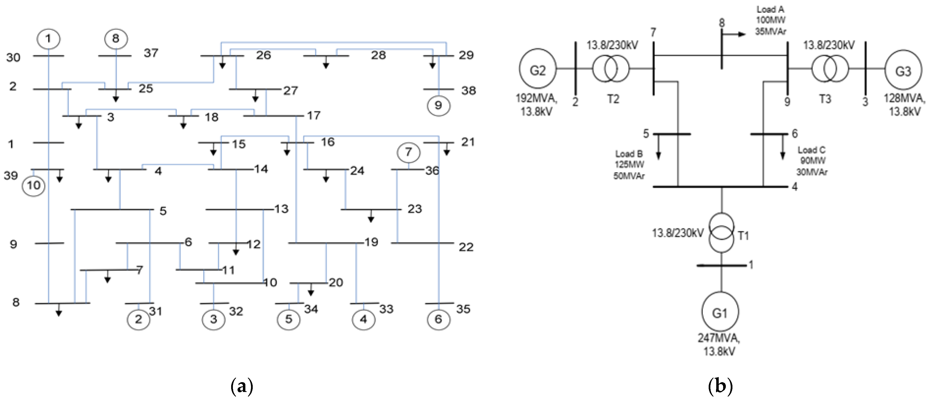
Two test systems are employed to validate the proposed online transient stability simulation approach. The first test system is the IEEE 9 bus system, which consists of nine bus and three machines. The second test system is the IEEE 39 bus system, which consists of 39 bus and 10 machines. The loads are modeled as constant impedances in the time domain simulation. The generators are represented by a two-axis fourth-order model. They all have a Type_1 excitation and voltage regulation system as well as a turbine/governor model. Figure 3 shows the Single line diagrams of both test system. Dynamic data of all the machines with in both test cases are given in Appendix A.
3.1.2. Simulation Cases
For the purpose of testing the proposed power system transient stability simulation method, three-phase bus faults are simulated for both systems. Three-phase short-circuit faults at bus 1 for IEEE 9 bus and at bus 31 for 39 bus test systems are considered during simulation. A susceptance of 10−10 is enough to bring zero-impedance bus faults [26].
3.1.3. Simulation Setup
Simulations were carried out on a standard laptop with the following characteristics: Intel CTM i5-5200U CPU @ 2.20 GHz 2.20 GHz, 8 GB RAM, running on a 64-bit operating system, with a x64-based processor. The time domain simulations were carried out using the simulation tools/codes developed based on the proposed AsDTM on MATLAB R2017b [27]. MATPOWER 7.1 [28] version software was utilized. The CPU times included all steps of the simulation processes. MATPOWER is open-source power simulation software, used for power flow analysis and run on a MATLAB environment. This power system analysis software does not employ a graphical representation of a power system. Instead, the power system data were prepared in a table format specific to MATPOWER. Any functions of the MATPOWER can easily be accessed by functions developed on MATLAB editor. These include MATLAB functions that load and call for dynamic and static data file of simulation cases (case file), MATPOWER output interface functions, functions for initializing dynamic systems, model libraries for all dynamic systems, solver functions file (algorithms for computation), and functions for plotting simulation results. Power flow analysis was performed using MATPOWER.
3.2. Simulation Results and Discussion
For validating the proposed AsDTM-based power system transient stability simulation, three-phase short-circuit faults on bus 2 of IEEE 9 bus and on bus 31 of 39 bus test systems at 0.6 s and cleared after 0.2 s were simulated. In each case, the accuracy and performance of the proposed method was validated using the transient stability simulation results based on the traditional numerical method (fourth-order Range–Kutta (Rk4) with step size h = 0.001 s) and total time cost (time for TS simulation) as benchmarks. For this simulation purpose, differential transformation (DT) order k = 7 for IEEE 9 bus and k = 10 for 39 bus test systems were used with both DTM and AsDTM simulation methods.
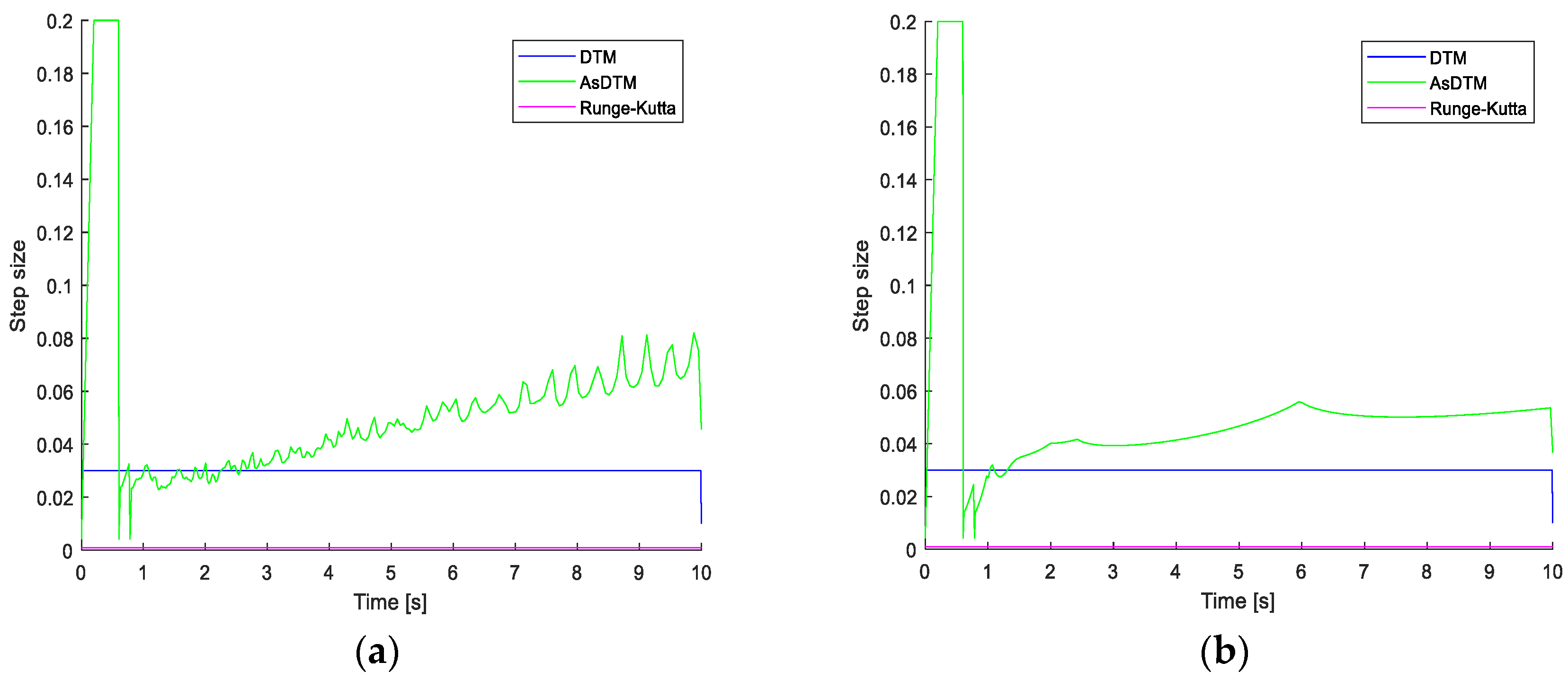
Figure 4 shows the step-size variation of the AsDTM-based transient stability simulation under admissible local error of 10−6. The step size varies adaptively between hmin = 0.00425 s and hmax = 0.2 s. The average step size h is equal to 0.01. For the DTM-based simulation, this average h = 0.01 was used as a fixed step size, shown in Figure 4.
Figure 3.
One-line diagram of (a) New England 39 bus system; (b) IEEE 9 bus system [29].
Figure 3.
One-line diagram of (a) New England 39 bus system; (b) IEEE 9 bus system [29].

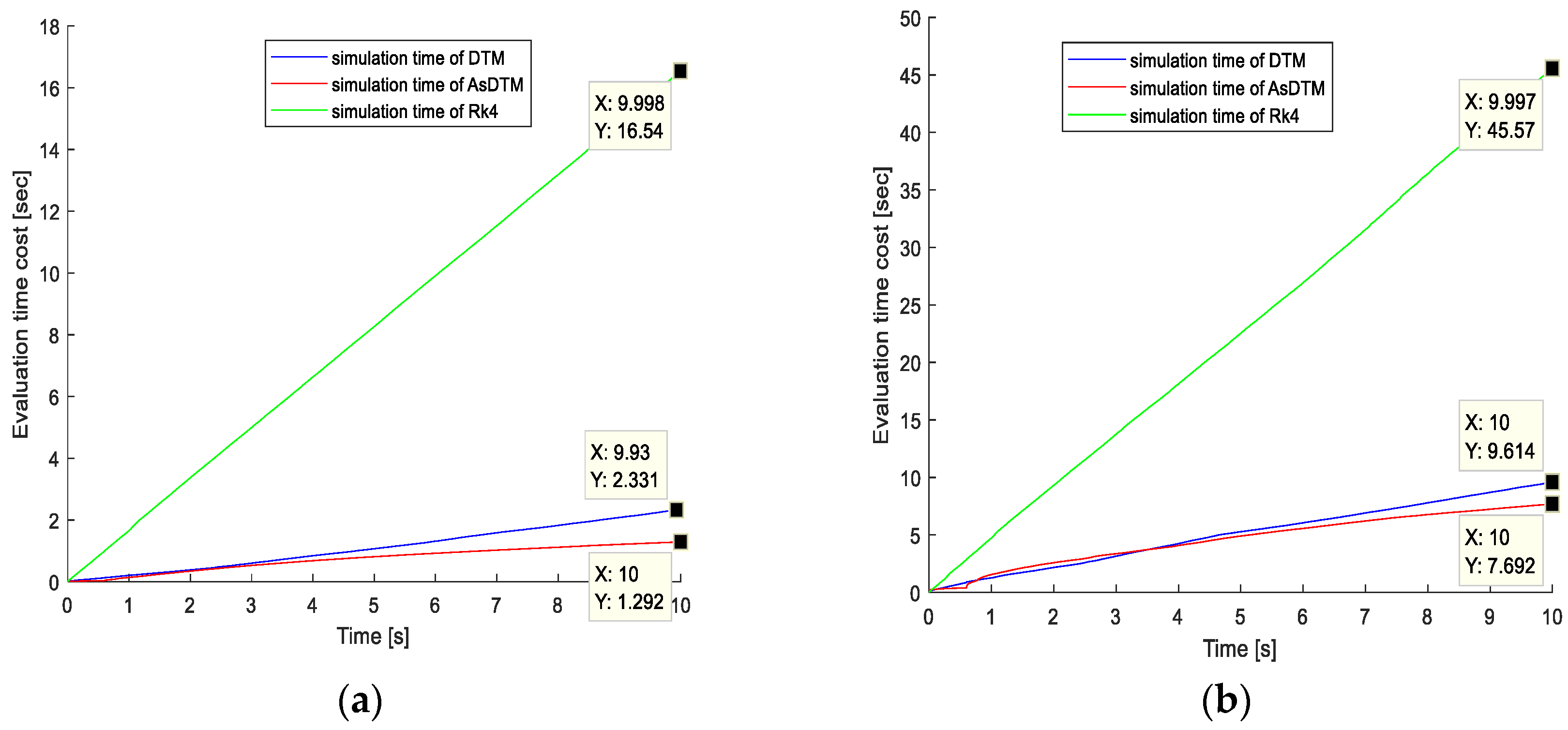
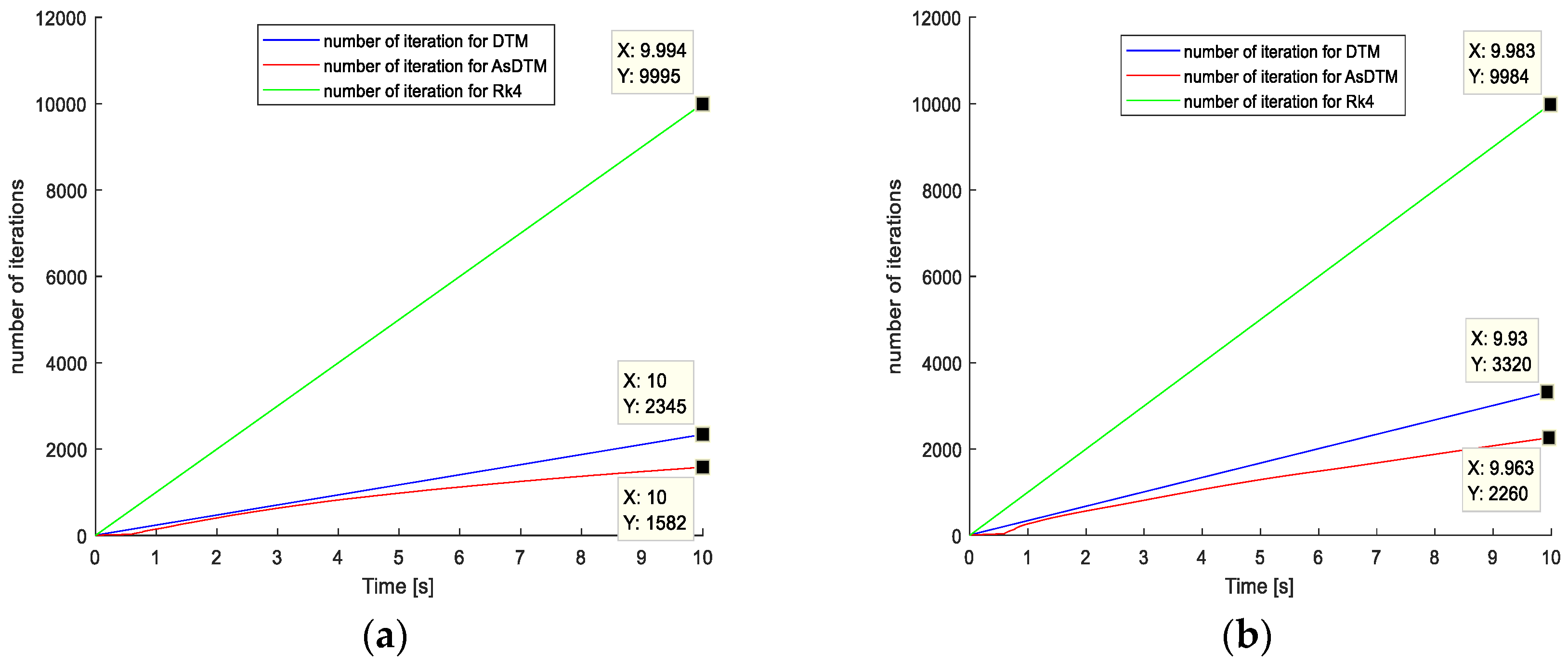
From Figure 5a,b and Figure 6a,b, we can observe the number of iterations and simulation time requirement relationships among AsDTM, DTM, and Rk4 simulation methods, respectively. The total number of iterations for simulating three-phase fault cleared after 0.2 s using Rk4, DTM, and AsDTM methods are 9995, 2345, and 1582 for the IEEE 9 bus test system and 9984, 3320, and 2260 for the IEEE 39 bus test system, respectively. Similarly, the total simulation time cost for the same case using Rk4, DTM, and AsDTM methods are 16.54 s, 2.331 s, and 1.292 s, for the IEEE 9 bus test system and 45.57 s, 9.614 s, and 7.692 for the IEEE 39 bus test system, respectively, from the simulation results shown in Figure 5 and Figure 6.
- DTM-based simulation: The proposed AsDTM improved/reduced the total simulation time cost and total number of iterations by 20% and 31.93% for the IEEE 39 bus test system and improved/reduced the total simulation time cost and total number of iterations by 44.57% and 32.54% for the IEEE 9 bus test system, respectively.
- Rk4-based simulation: The proposed AsDTM improved/reduced the total simulation time cost and total number of iterations by 83% and 77.36% for the IEEE 39 bus test system and improved/reduced the total simulation time cost and total number of iterations by 92% and 84% for the IEEE 9 bus test system, respectively.
Therefore, we can conclude that the proposed AsDTM-based power system transient stability simulation method increases simulation speed by 20–44.57% and 83–92% when compared with the DTM- and Rk4-based simulations, respectively.
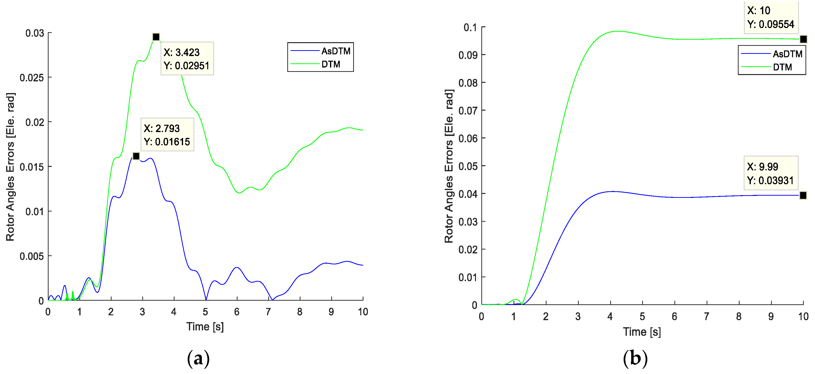
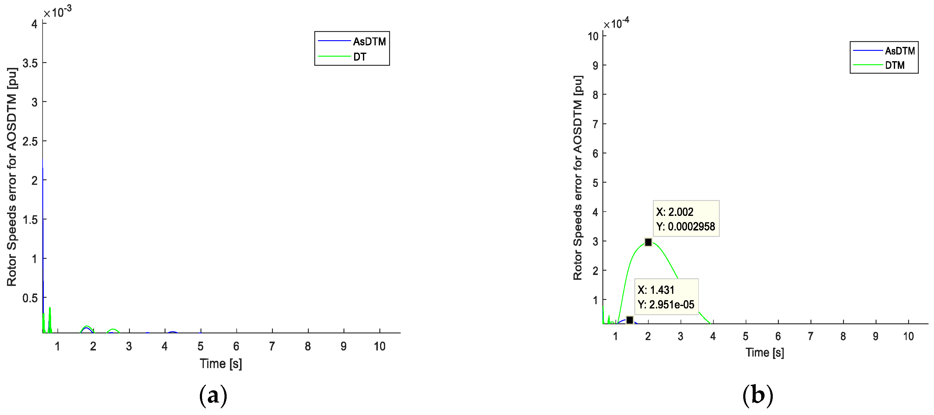
Figure 7a,b and Figure 8a,b, show the rotor angle and speed errors simulation results. Error results relationships among AsDTM and DTM simulation methods are given in Table 1 below.
From the simulation results of Figure 7a,b and Figure 8a,b and Table 1, compared with the DTM-based simulation, the proposed AsDTM-based power system transient stability simulation improves rotor angle error by 45.27% and 58.85% and improves rotor speed error by 90% for IEEE 9 and IEEE 39 test systems, respectively.
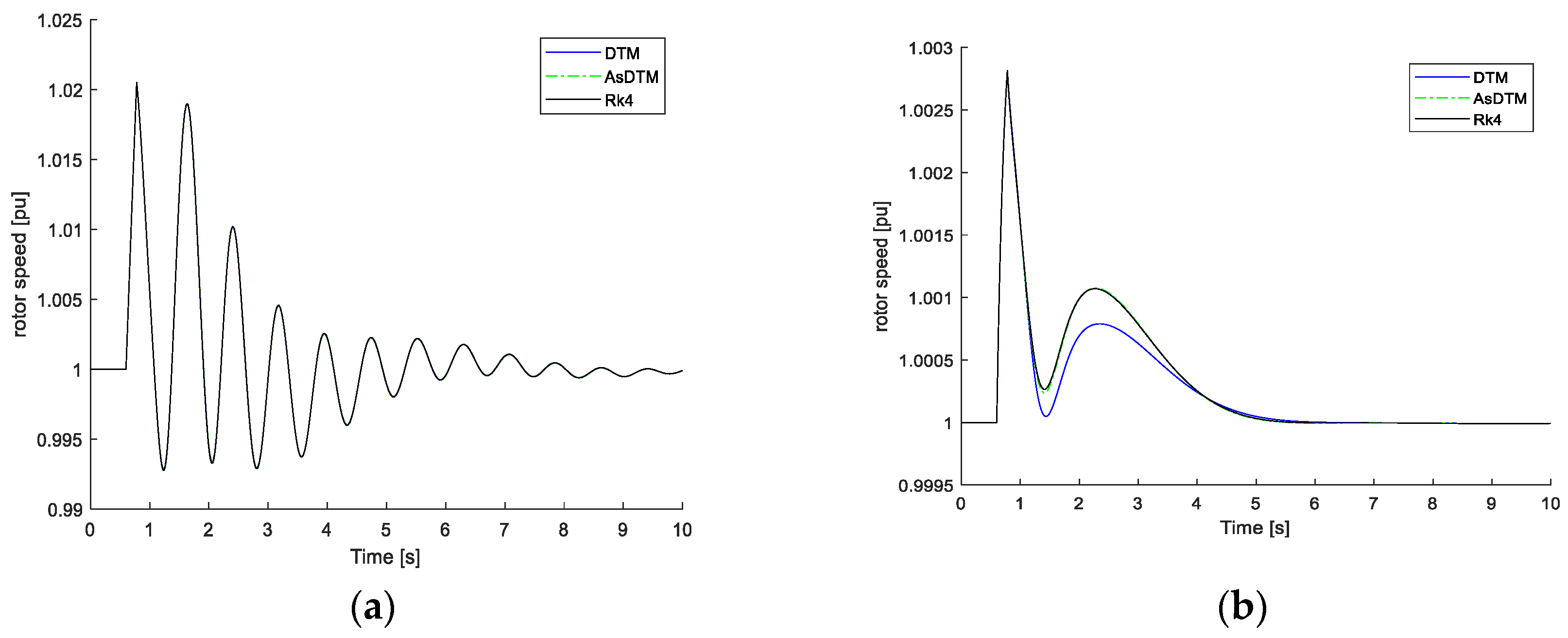
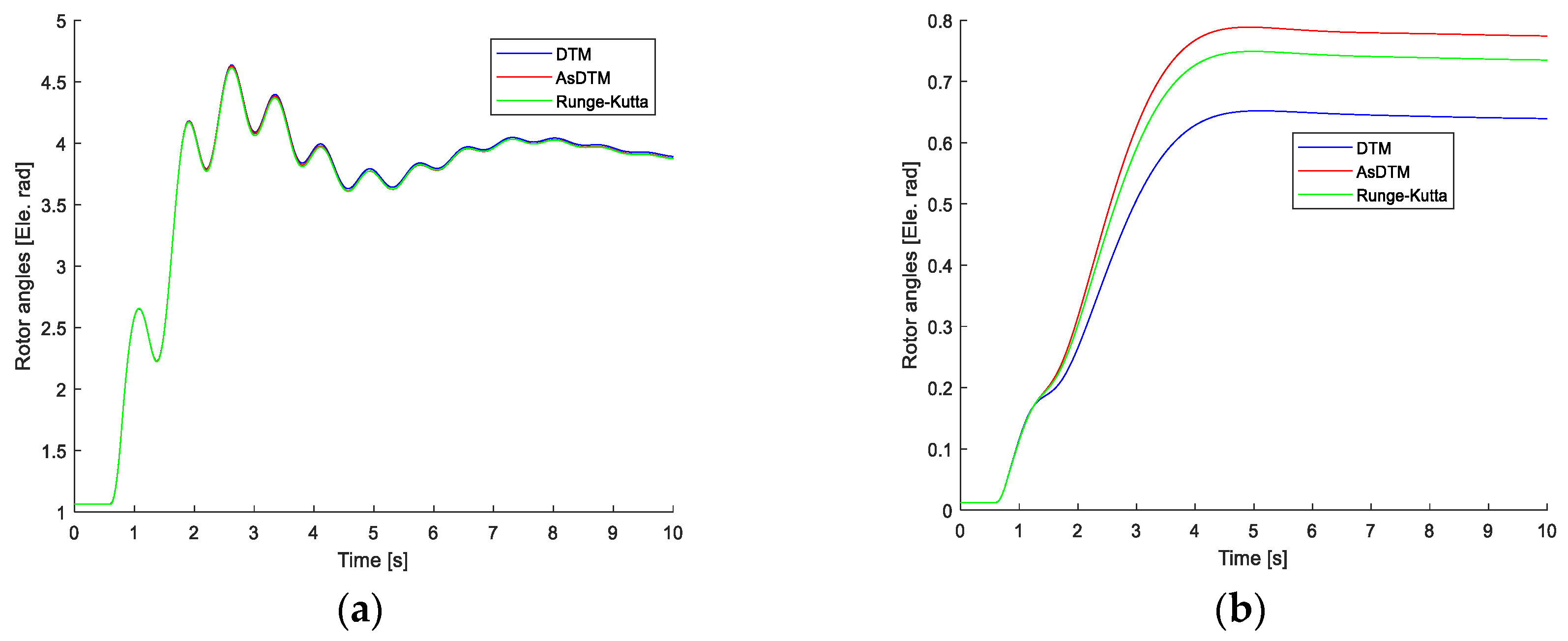
Figure 9a,b and Figure 10a,b, represent the rotor angle and speed simulation results, where the quality of results obtained with AsDTM and DTM methods used the convergence criterion, the measure of which is the concurrency time of curves corresponding to two compared solutions. The best convergence was found for the AsDTM results. This implies that the AsDTM-based simulation gives more accurate results. However, since the shapes of the trajectories obtained by both DTM and AsDTM methods were the same as the reference trajectory obtained by the Rk4 method, we can conclude that both DTM and AsDTM methods are numerically stable.
4. Conclusions and Future Work
In this paper, an AsDTM-based fast and accurate power system transient stability simulation is proposed. The validity of the method was proven successful by applying it to IEEE 3 machines 9 bus and New England 10 machines 39 bus test systems. The power system transient stability simulation results are presented in the figures for the given admissible local errors and fault locations. The results show that the method works successfully in handling the complex nonlinear power system differential algebraic equations with a reduced computation time cost and a wide interval of convergence.
As described in Section 4 above, the proposed approach improves the accuracy of simulation results by 45.27% to 58.85% and by 90% for IEEE 9 and IEEE 39 test systems, respectively, compared with the classical DTM. Furthermore, the proposed method also increases the simulation speed by 20–44.57% when compared with the classical DTM-based simulation. Therefore, by adaptively varying the step size of the differential transformation method, the speed and accuracy of the power system transient stability simulation is improved when compared with the classical DTM. Similarly, the simulation speed is improved significantly (by 83–92%) when compared with the traditional Rk4 simulation method. In general, the simulation results show that the proposed method is relatively accurate, fast, and efficient when compared with the classical fixed-step DTM-based simulation method. Therefore, we can conclude that the proposed method can be applied as an online transient stability simulation tool. Practical implementation of the proposed method in real-world power system operations is possible without any technical limitation, because the method is flexible enough to accommodate system models with any detail, and only requires the most recent snapshot from SCADA systems, generators, and their controllers’ dynamic data.
Extending the approach for power system online contingency screening, which is the first stage of the online DSA session, will be our next focus of research.
Author Contributions
Conceptualization. methodology, software, formal analysis, investigation, resources, data curation, writing—original draft preparation, writing—review and editing, by T.L.K. Validation, visualization by T.L.K. and F.S. Supervision, project administration, by F.S. All authors have read and agreed to the published version of the manuscript.
Funding
This research received no external funding.
Data Availability Statement
All power flow data for the test cases are taken from Matpower software package cited in the reference. All dynamic data used for machines and their controllers given in the Appendix A Simulation codes are developed in Matlab 2017b environment.
Conflicts of Interest
The authors declare no conflict of interest.
Appendix A
IEEE 9 Bus and New England 39 Bus Test Systems Generators and their controller’s Data.

Table A1.
New England 39 bus test system generator data 1 [25].
Table A1.
New England 39 bus test system generator data 1 [25].
| Bus # | Xd | Xq | X’d | X’q | Rs | T’do | T’qo | H | Dg |
|---|---|---|---|---|---|---|---|---|---|
| 30 | 0.1000 | 0.0690 | 0.0310 | 0.0690 | 0.0002 | 10.200 | 0.020 | 42.000 | 0.0535 |
| 31 | 0.2590 | 0.2820 | 0.0700 | 0.1700 | 0.0002 | 6.5600 | 1.5000 | 30.300 | 0.0194 |
| 32 | 0.2500 | 0.2370 | 0.0530 | 0.0880 | 0.0002 | 5.7000 | 1.5000 | 35.500 | 0.06783 |
| 33 | 0.2620 | 0.2580 | 0.0440 | 0.1660 | 0.0002 | 5.6900 | 1.5000 | 28.500 | 0.01815 |
| 34 | 0.6700 | 0.6200 | 0.1320 | 0.1660 | 0.0002 | 5.4000 | 0.4400 | 26.000 | 0.0331 |
| 35 | 0.2540 | 0.2410 | 0.0500 | 0.0810 | 0.0002 | 7.3000 | 0.4000 | 35.00 | 0.06783 |
| 36 | 0.2950 | 0.2920 | 0.0490 | 0.1860 | 0.0002 | 5.6600 | 1.5000 | 26.500 | 0.01815 |
| 37 | 0.2900 | 0.2800 | 0.0570 | 0.0910 | 0.0010 | 6.7000 | 0.4100 | 24.300 | 0.0331 |
| 38 | 0.2110 | 0.2050 | 0.0570 | 0.0590 | 0.0002 | 4.7900 | 1.9600 | 34.500 | 0.06783 |
| 39 | 0.0200 | 0.0190 | 0.0060 | 0.0080 | 0.0002 | 7.0000 | 0.7000 | 31.000 | 0.01940 |
Table A2.
New England system generator controller’s data [26].
Table A2.
New England system generator controller’s data [26].
| Bus # | Ke | Te | Aexc | Bexc | Ur_max | Ur_min | Ka | Ta | Kf | Tf | Tch | Tg | Rg |
|---|---|---|---|---|---|---|---|---|---|---|---|---|---|
| 30 | 1.0000 | 0.2500 | 0.0039 | 1.55 | 10 | −10 | 20 | 0.06 | 0.04 | 1.0 | 0.1 | 0.05 | 0.05 |
| 31 | 1.0000 | 0.4100 | 0.0039 | 1.55 | 10 | −10 | 20 | 0.05 | 0.06 | 0.5 | 0.1 | 0.05 | 0.05 |
| 32 | 1.0000 | 0.5000 | 0.0039 | 1.55 | 10 | −10 | 20 | 0.06 | 0.08 | 1.0 | 0.1 | 0.05 | 0.05 |
| 33 | 1.0000 | 0.5000 | 0.0039 | 1.55 | 10 | −10 | 20 | 0.06 | 0.08 | 1.0 | 0.1 | 0.05 | 0.05 |
| 34 | 1.0000 | 0.7900 | 0.0039 | 1.55 | 10 | −10 | 20 | 0.02 | 0.03 | 1.0 | 0.1 | 0.05 | 0.05 |
| 35 | 1.0000 | 0.4700 | 0.0039 | 1.55 | 10 | −10 | 20 | 0.02 | 0.08 | 1.25 | 0.1 | 0.05 | 0.05 |
| 36 | 1.0000 | 0.7300 | 0.0039 | 1.55 | 10 | −10 | 20 | 0.02 | 0.03 | 1.0 | 0.1 | 0.05 | 0.05 |
| 37 | 1.0000 | 0.5300 | 0.0039 | 1.55 | 10 | −10 | 20 | 0.02 | 0.09 | 1.26 | 0.1 | 0.05 | 0.05 |
| 38 | 1.0000 | 1.4000 | 0.0039 | 1.55 | 10 | −10 | 20 | 0.02 | 0.03 | 1.0 | 0.1 | 0.05 | 0.05 |
| 39 | 0.0200 | 0.0190 | 0.0060 | 0.0080 | 0.0002 | 7.0 | 0.70 | 31.0 | 0.01940 |
Table A3.
IEEE 9 bus test system generator data.
| Bus # | Xd | Xq | X’d | X’q | Rs | T’do | T’qo | H | Dg |
|---|---|---|---|---|---|---|---|---|---|
| 1 | 0.146 | 0.0969 | 0.0608 | 0.0969 | 0.004 | 8.96 | 0.31 | 23.000 | 0.0151 |
| 2 | 0.8958 | 0.8648 | 0.1198 | 0.1969 | 0.0026 | 6.00 | 0.535 | 6.400 | 0.001 |
| 3 | 1.3125 | 1.2578 | 0.1813 | 0.25 | 0.0035 | 5.890 | 0.6 | 3.010 | 0.0058 |
Table A4.
IEEE 9 bus test system generator controller’s data.
| Bus # | Ke | Te | Aexc | Bexc | Ur_max | Ur_min | Ka | Ta | Kf | Tf | Tch | Tg | Rg |
|---|---|---|---|---|---|---|---|---|---|---|---|---|---|
| 1 | 1.0000 | 0.3140 | 0.0039 | 1.55 | 3 | −3 | 20.0 | 0.20 | 0.0630 | 0.350 | 0.10 | 0.05 | 0.05 |
| 2 | 1.0000 | 0.3140 | 0.0039 | 1.55 | 3 | −3 | 20.0 | 0.20 | 0.0630 | 0.350 | 0.1 | 0.05 | 0.05 |
| 3 | 1.0000 | 0.3140 | 0.0039 | 1.55 | 3 | −3 | 20.0 | 0.20 | 0.0630 | 0.350 | 0.1 | 0.05 | 0.05 |
References
- Sarajcev, P.; Kunac, A.; Petrovic, G.; Despalatovic, M. Power System Transient Stability Assessment Using Stacked Autoencoder and Voting Ensemble. Energies 2021, 14, 3148. [Google Scholar] [CrossRef]
- Perilla, A.; Papadakis, S.; Rueda Torres, J.L.; van der Meijden, M.; Palensky, P.; Gonzalez-Longatt, F. Transient Stability Performance of Power Systems with High Share of Wind Generators Equipped with Power-Angle Modulation Controllers or Fast Local Voltage Controllers. Energies 2020, 13, 4205. [Google Scholar] [CrossRef]
- Tina, G.M.; Maione, G.; Licciardello, S. Evaluation of Technical Solutions to Improve Transient Stability in Power Systems with Wind Power Generation. Energies 2022, 15, 7055. [Google Scholar] [CrossRef]
- Kundur, P.; Paserba, J.; Ajjarapu, V.; Andersson, G.; Bose, A.; Canizares, C.; Vittal, V. IEEE/CIGRE Joint Task Force on Stability Terms and Definitions, Definition and Classification of Power System Stability. IEEE Trans. Power Syst. 2004, 19, 1387–1401. [Google Scholar]
- Stott, B. Power system Dynamic response calculation. Proc. IEEE 1979, 67, 219–241. [Google Scholar] [CrossRef]
- Chow, J.H. Power System Coherency and Model Reduction; Springer: New York, NY, USA, 2013. [Google Scholar]
- Osipov, D.; Sun, K. Adaptive nonlinear model reduction for fast power system simulation. IEEE Trans. Power Syst. 2018, 33, 6746–6754. [Google Scholar] [CrossRef]
- Milano, F. Power System Modeling and Scripting; Springer Science and Business Media: Berlin/Heidelberg, Germany, 2010. [Google Scholar]
- Gurrala, G.; Dimitrovski, A.; Pannala, S.; Simunovic, S.; Starke, M. Parareal in Time for Fast Power System Dynamic Simulations. IEEE Trans. Power Syst. 2015, 31, 1820–1830. [Google Scholar] [CrossRef]
- Zadkhast, S.; Jatskevich, J.; Vaahedi, E. A multi-decomposition approach for accelerated time domain simulation of transient stability problems. IEEE Trans. Power Syst. 2015, 30, 2301–2311. [Google Scholar] [CrossRef]
- Aristidou, P.; Fabozzi, D.; Cutsem, T.V. Dynamic Simulation of Large Scale Power Systems Using a Parallel Schur-Compelement_Based Decomposition Method. IEEE Trans. Parallel Distrib. Syst. 2014, 25, 2561–2570. [Google Scholar] [CrossRef]
- Liu, C.; Wang, B.; Sun, K. Fast power system simulation using semi-analytical solutions based on Pade approximation. In Proceedings of the 2017 IEEE Power & Energy Society General Meeting, Chicago, IL, USA, 16–20 July 2017; pp. 1–5. [Google Scholar]
- Liu, C.; Wang, B.; Sun, K. Fast power system Dynamic Simulation Using Continued Fractions. IEEE Access 2018, 6, 62687–62698. [Google Scholar] [CrossRef]
- Wang, B.; Duan, N.; Sun, K. A Time-Power Series Based Semi-Analytical Approach for Power System Simulation. IEEE Trans. Power Syst. 2019, 34, 841–851. [Google Scholar] [CrossRef]
- Liu, Y.; Sun, K.; Yao, R.; Wang, B. Power System Time Domain Simulation Using a Differential Transformation Method. IEEE Trans. Power Syst. 2019, 34, 3739–3748. [Google Scholar] [CrossRef]
- Liu, Y.; Sun, K. Power System Simulation Using a Differential Transformation Method. Ph.D. Thesis, University of Tennessee, Knoxville, TN, USA, 2022. Available online: https://trace.tennessee.edu/utk_graddiss/7073 (accessed on 28 August 2022).
- Sanchez-Gasca, J.J.; D’aquila, R.; Price, W.W.; Paserba, J.J. Variable time step, implicit integration for extended-term power system dynamic simulation. In Proceedings of the Power Industry Computer Applications Conference, Salt Lake City, UT, USA, 7–12 May 1995. [Google Scholar] [CrossRef]
- Kim, S.; Overbye, T.J. Optimal Subinterval Selection Approach for Power System Transient Stability Simulation. Energies 2015, 8, 11871–11882. [Google Scholar] [CrossRef]
- Laugier, A.J.C. Adaptive Time Step for Fast Converging Dynamic Simulation System. In Proceedings of the IEEE/RSJ International Conference on Intelligent Robots and Systems, IROS ’96, Osaka, Japan, 8 November 1996. [Google Scholar] [CrossRef]
- Liu, Y.; Sun, K. Solving Power System Differential Algebraic Equations Using Differential Transformation. IEEE Trans. Power Syst. 2020, 35, 2289–2299. [Google Scholar] [CrossRef]
- El-Zahar, E.R. An Adaptive Step-Size Taylor Series Based Method and Application to Nonlinear Biochemical Reaction Model. Trends Appl. Sci. Res. 2012, 7, 901–912. [Google Scholar]
- El-Zahar, E.R. Applications of Adaptive Multi Step Differential Transform Method to Singular Perturbation Problems Arising in Science and Engineering. Appl. Math. Inf. Sci. 2015, 9, 223–232. [Google Scholar] [CrossRef]
- Ahmet, G.; Mehmet, M.; Ahmet, Y. Adaptive multi-step differential transformation method to solving nonlinear differential equations. Math. Comp. Mod. Sci. 2012, 55, 761–769. [Google Scholar]
- Bég, O.A.; Keimanesh, M.; Rashidi, M.M.; Davoodi, M.; Branch, S.T. Multi-step DTM Simulation of Magneto-Peristaltic Flow of a Conducting Williamson Viscoelastic Fluid. Int. J. Appl. Math Mech. 2013, 9, 22–40. [Google Scholar]
- Pukhov, E.; Georgii, G. Differential transformation method and circuit theory. Int. J. Circuit Theory Appl. 1982, 10, 265–276. [Google Scholar] [CrossRef]
- Available online: http://www.esat.kuleuven.be/electa/teaching/matdyn/ (accessed on 26 May 2020).
- MATLAB, T.M.I.2017b; The MathWorks Inc.: Natick, MA, USA, 2017.
- Zimmerman, R.D.; Murillo-Sanchez, C.E.; Thomas, R.J. MATPOWER: Steady-State Operations, Planning, and Analysis Tools for Power Systems Research and Education. IEEE Trans. Power Syst. 2011, 26, 12–19. [Google Scholar] [CrossRef]
- Yang, D. Power System Dynamic Security Analysis via Decoupled Time Domain Simulation and Trajectory Optimization; Iowa State University: Ames, IA, USA, 2006. [Google Scholar]
Figure 1.
Flowchart of AsDTM-based fast power system transient stability simulation method.

Figure 2.
Recursive process to solve power series coefficients (source: [20]), where X(k) represents and j = 1, 2, 3 … m.
Figure 2.
Recursive process to solve power series coefficients (source: [20]), where X(k) represents and j = 1, 2, 3 … m.

Figure 4.
Step-size variations during simulation for IEEE (a) 9 bus and (b) 39 bus test systems.

Figure 5.
Simulation time cost for IEEE (a) 9 bus and (b) 39 bus test systems.

Figure 6.
Number of iterations for IEEE (a) 9 bus and (b) 39 bus test systems.

Figure 7.
Rotor angle error for IEEE (a) 9 bus and (b) 39 bus test systems.

Figure 8.
Rotor speed error for IEEE (a) 9 bus and (b) 39 bus test systems.

Figure 9.
Rotor speed simulation for IEEE (a) 9 bus and (b) 39 bus test systems.

Figure 10.
Rotor angle simulation for IEEE (a) 9 bus and (b) 39 bus test systems.

Table 1.
Rotor angle and speed errors simulation results relationships.
| Method | Max Error | |||
|---|---|---|---|---|
| IEEE 9 | IEEE 39 | IEEE 9 | IEEE 39 | |
| Rotor Angle (rad) | Rotor Speed (pu) | |||
| AsDTM | 0.01615 | 0.03931 | 0.00005 | 0.00002951 |
| DTM | 0.02951 | 0.09554 | 0.0005 | 0.0002958 |
Disclaimer/Publisher’s Note: The statements, opinions and data contained in all publications are solely those of the individual author(s) and contributor(s) and not of MDPI and/or the editor(s). MDPI and/or the editor(s) disclaim responsibility for any injury to people or property resulting from any ideas, methods, instructions or products referred to in the content. |
© 2023 by the authors. Licensee MDPI, Basel, Switzerland. This article is an open access article distributed under the terms and conditions of the Creative Commons Attribution (CC BY) license (https://creativecommons.org/licenses/by/4.0/).
Share and Cite
MDPI and ACS Style
Kumissa, T.L.; Shewarega, F. Fast Power System Transient Stability Simulation. Energies 2023, 16, 7157. https://doi.org/10.3390/en16207157
AMA Style
Kumissa TL, Shewarega F. Fast Power System Transient Stability Simulation. Energies. 2023; 16(20):7157. https://doi.org/10.3390/en16207157
Chicago/Turabian StyleKumissa, Teshome Lindi, and Fekadu Shewarega. 2023. "Fast Power System Transient Stability Simulation" Energies 16, no. 20: 7157. https://doi.org/10.3390/en16207157
Note that from the first issue of 2016, this journal uses article numbers instead of page numbers. See further details here.