Article

Hammerstein–Wiener Model Identification for Oil-in-Water Separation Dynamics in a De-Oiling Hydrocyclone System

1
AAU Energy, Aalborg University, Niels Bohrs Vej 8, 6700 Esbjerg, Denmark
2
Department of Chemical and Materials Engineering, University of Alberta, Edmonton, AB T6G 2G6, Canada
*
Author to whom correspondence should be addressed.
Energies 2023, 16(20), 7095; https://doi.org/10.3390/en16207095
Submission received: 23 August 2023 / Revised: 9 October 2023 / Accepted: 11 October 2023 / Published: 14 October 2023
(This article belongs to the Special Issue Subsurface Energy and Environmental Protection)

Abstract

:
To reduce the environmental impact of offshore oil and gas, the hydrocarbon discharge regulations tend to become more stringent. One way to reduce the oil discharge is to improve the control systems by introducing new oil-in-water (OiW) sensing technologies and advanced control. De-oiling hydrocyclones are commonly used in offshore facilities for produced water treatment (PWT), but obtaining valid control-oriented models of hydrocyclones has proven challenging. Existing control-oriented models are often based on droplet trajectory analysis. While it has been demonstrated that these models can fit steady-state separation efficiency data, the dynamics of these models have either not been validated experimentally or only describe part of the dynamics. In addition to the inlet OiW concentration, they require the droplet size distribution to be measured, which complicates model validation as well as implementation. This work presents an approach to obtain validated nonlinear models of the discharge concentration, separation efficiency, and discharge rate, which do not require the droplet size distribution to be measured. An exhaustive search approach is used to identify control-oriented polynomial-type Hammerstein–Wiener (HW) models of de-oiling hydrocyclones based on concentration measurements from online OiW monitors. To demonstrate the effectiveness of this modeling approach, a PI controller is designed using the Skogestad internal model control (SIMC) tuning rules to control the discharge OiW concentration directly. The identification experiment emulates an offshore PWT system with installed OiW monitors, which is realistic with the legislative incentive to include online OiW discharge measurements. The proposed approach could enable the application of OiW-based control on existing offshore PWT facilities, resulting in improved de-oiling performance and reduced oil discharge.

Graphical Abstract

1. Introduction

Oil and gas production will remain a vital energy source during the transition toward green energy. Besides greenhouse gas emissions, oil and gas production pollutes through accidental oil spills and the discharge of produced water (PW). Currently, the Oslo and Paris Commission’s (OSPAR) regulation for the discharge of PW with dispersed hydrocarbon is 30 mg/L (approximately 30 ppm). The oil-in-water (OiW) concentration is measured with the current OSPAR reference method, which is an offline lab-based method using a gas chromatography analyzer with a flame ionization detector (GC-FID) [1]. Though most oil and gas installations complied with the concentration requirement on average, the annual hydrocarbon discharge in the North Sea amounted to 4000 tonnes between 2009 and 2019 [2].
Besides the OSPAR recommendations, the Danish Environmental Protection Agency also restricts the total annual hydrocarbon discharge quantity to be below 222 tonnes. To meet this goal, each operator has a discharge permit specifying how much of the 222 tonnes they are allowed to discharge each year. The operators are required to install OiW measuring equipment and flow meters to determine the discharge quantity [1]. With large quantities of PW, the total discharge can come close to the limit, as in 2016, where the dispersed discharge in the Danish region reached 200 tonnes [3]. As the oil fields mature, more water is produced, which can lead to larger discharge quantities and, additionally, discharge legislation may become more stringent. One way to reduce the discharge is to improve the control of the separation process.
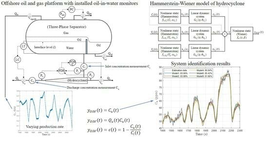
The offshore oil and gas separation installations typically consist of several three-phase separators, where the incoming well stream is separated into water, oil, and gas, after which each phase undergoes further treatment. Hydrocyclones are commonly deployed to further reduce the oil residuals in the PW leaving the water outlet of the separator vessels. A piping and instrumentation diagram (P&ID) of a typical configuration with a coupled three-phase separator and a hydrocyclone system is shown in Figure 1.
The conical shape of the hydrocyclone wall delivers the centripetal force needed to generate a vortex flow, and the lighter dispersed oil droplets migrate toward the hydrocyclone’s axial center due to the density difference between oil and water. The accumulated oil-rich stream is rejected through the overflow outlet, while the cleaned water exits through the underflow outlet. The de-oiling performance of hydrocyclone is sensitive to the operating condition, particularly to the feeding flow rate, flow split, inlet concentration, oil droplet size distribution, etc. [4,5]. Some control system is thereby needed to maintain the hydrocyclone in a reasonable operating range to gain a high separation performance. One of the most common solutions is to maintain the flow split according to the vendor’s recommendation, where the flow split is defined as:
F s = Q o Q i ,
where Q o / Q i is the overflow/inflow volumetric flow rate. In practice, the flow split is controlled by the pressure drop ratio (PDR), which is defined as the ratios between the pressure drop from inlet to overflow and the pressure drop from inlet to underflow, i.e.,
P D R = P i P o P i P u .
As illustrated in Figure 1, the control valve ( V o ) located at the hydrocyclone’s overflow (oil-rich) outlet is used to control the PDR. The upstream separator’s water level is controlled by manipulating the control valve ( V u ) located at the hydrocyclone’s underflow (water-rich) outlet. The PDR is used as one of the controlled variables (CVs) in the existing hydrocyclone control solutions [5,6]. However, a clear coupling between the level control loop and PDR control loop has been observed but not systematically handled, except for some empirical designs in the existing control solutions, mainly due to the fact that each control loop is developed as a standalone PID type of solution. Furthermore, by deploying online OiW monitors in the process, it has been discovered that the correlation of PDR with OiW concentration at the underflow outlet is not static, i.e., it is temporally dependent on the operating condition [7,8]. Thereby, a natural question occurs: how can the available OiW measurement be included in the hydrocyclone control to achieve direct control of hydrocarbon discharge in the produced water treatment (PWT) process? Though some operators have already installed online OiW monitors in their PWT processes, to the authors’ knowledge, there is no report about existing control systems that use online OiW measurements as a feedback signal yet.
One obstacle in getting an OiW-based control solution is the lack of some control-oriented model which can describe the key OiW separation dynamics inside the hydrocyclone in a reasonably precise manner. Computational Fluid Dynamics (CFD) modeling of hydrocyclone systems has been used extensively to design and simulate hydrocyclone systems, e.g., to investigate the effect of different geometries and operating conditions on separation efficiency [9,10,11,12,13]. However, these CFD models are too complicated to support feedback control design, which often requires some simple control-oriented mathematical models.
Unlike complicated CFD-based models, Wolbert et al. [14] presented a simple model describing the hydrocyclone’s separation efficiency using droplet trajectory analysis. The trajectories are defined by the tangential, axial, and radial velocity fields of the carrier (continuum) phase and the (dispersion) droplets’ phase, subject to the assumption of no droplet coalescence or break-ups. The hydrocyclone’s separation efficiency can then be calculated based on the grade efficiency if the droplet size distribution can be known. Similar approaches have been examined by Caldenley et al. [15] and Amini et al. [16], and some promising results have been reported on experimental steady-state data. Bram et al. [17] combined a flow-resistance model with an extended version of the droplet trajectory model by Wolbert et al. [14] such that the coefficients describing the axial velocity distribution are calculated by considering boundary conditions. The model showed some similarities with dynamic experimental data, and model performance improved after placing the OiW monitors closer to the sampling probes and actively controlling the sidestream flow rate to a constant set point [4]. The model achieved a better match to the steady-state efficiency curve, but the dynamic characteristics still need to be improved. Vallabhan et al. [6] presented a droplet trajectory model, where the axial velocity was modeled as a flow through a converging nozzle. This model was compared with a set of steady-state experimental data from Meldrum et al. [5] and achieved a reasonable fit to the efficiency as a function of normalized inlet flow rate. The droplet size distribution was, however, unknown in Meldrum et al. [5], and the authors assumed a droplet size distribution with diameters ranging from 5 to 60 µm. The authors approximated the separation efficiency for a fixed underflow valve opening degree as a second-order polynomial function of the overflow flow rate and derived mass balances to describe the separation dynamics. A PI controller was developed using the Skogestad internal model control (SIMC) tuning rules, and later, a sliding mode, feedback linearization, feedforward, cascade, and model predictive controller (MPC) were designed to track a constant discharge concentration reference in simulation [6,18,19]. These models have proven to be capable of representing the steady-state efficiency behavior of hydrocyclones, but the dynamic features have not been validated or have been insufficient to describe the data [4,6]. The lack of validation is likely due to the difficulty of measuring the droplet size distribution in a reliable online manner.
Nonlinear black-box models have mainly been used for control-oriented modeling of PDR. Hansen et al. [20] extended a state-space model from Durdevic et al. [21] with a non-linear static function on the overflow valve input to make the PDR model valid in a wider operating range. The resulting Hammerstein model was used to design a MPC for the level and PDR, which could better comply with the level constraints than the H controller presented by Durdevic et al. [21].
Motivated by these previous works, this paper intends to investigate models of the OiW separation dynamics inside the hydrocyclone system using Hammerstein–Wiener (HW) models based only on OiW concentration measurements. A similar idea can be found in our preliminary work in Jespersen et al. [22], where only the separation efficiency is defined as the CV of the developed model. In this work, the possible CV can be extended as the hydrocarbon discharge concentration and discharge rate as well.
The scientific contributions of this paper consist of: (i) a nonlinear HW model framework is proposed to describe the separation dynamics inside a de-oiling hydrocyclone system based on online (inlet and underflow outlet) OiW measurements; (ii) a data-driven system identification approach is employed to identify the specific HW model coefficients based on a dedicated experiment; and (iii) the benefit and usefulness of the proposed model are validated by a (OiW-based) quality control solution developed by SIMC tuning rules based on the obtained model. The experimental validation of the proposed model and method shows the promising potential to include the online OiW measurement into the feedback control to achieve direct and improved discharge quality control, thereby further mitigating the marine environmental pollution caused by the discharge of PW.

2. Materials and Methods

The definition and the motivation for three different OiW-based CVs are given in Section 2.1. The HW model structure and identification method are presented in Section 2.2. The experimental facility and the experiment design are outlined in Section 2.3, and the data preprocessing steps are described in Section 2.4. Finally, the approach used to determine the model orders is presented in Section 2.5.

2.1. Oil-in-Water Based Controlled Variables

To apply OiW-based control, CVs related to PW discharge must be defined. In the following, three potential CVs are presented.
Separation efficiency: PDR does not keep a constant proportional relationship with the separation efficiency, even subject to different steady-state conditions, while the time-varying (dynamic) separation efficiency, denoted as ϵ ( t ) , can be calculated using online OiW measurements as
ϵ ( t ) = 1 C u ( t ) C i ( t ) = 1 C r ( t ) ,
where C r ( t ) = C u ( t ) / C i ( t ) represents the OiW measurement at the underflow/inlet location at time t. Equation (3) is also referred to as the reduced efficiency equation [4]. A more realistic transient efficiency is given as
ϵ ( t ) = 1 C u ( t ) C i ( t δ t ( t ) ) ,
where δ t ( t ) is the transition time for the droplets to pass through the hydrocyclone body. The OiW dynamics (utility and technology dependent [23]) can only be considered relatively slow (e.g., in minutes) compared with the dynamics of droplets passing through the cyclone (e.g., in seconds), the δ t ’s impact can be ignored or regarded as a part of the model uncertainties.
Oil discharge rate: with the sheer volume of PW, the total discharge of oil can still be large, even with extremely low discharge concentrations. By deploying an OiW instrument and a flow meter at the water outlet of the hydrocyclone system, the total oil discharge rate, denoted as Q u , o i l ( t ) , can be defined as a new CV, i.e.,
Q u , o i l ( t ) = C u ( t ) Q u ( t ) ,
where C u ( t ) is the instantaneous underflow OiW concentration measurement and Q u ( t ) is the volumetric flow rate measured by the flowmeter.
Discharge concentration: the discharge concentration denoted as C u is a natural choice of CV to comply with the discharge concentration limits, as studied in [6,8,18,19].

2.2. Hammerstein–Wiener Nonlinear Model

As shown in Figure 2, a nonlinear HW model can be represented as a linear dynamic model sandwiched between two static/memory-less nonlinear functions. Without the output nonlinearity, the model simplifies to a Hammerstein model, while a linear dynamic system followed by a nonlinear static function is a Wiener model. Hammerstein, Wiener, and HW models have been widely used due to their relative simplicity and capability to describe many nonlinear dynamic systems [20,24,25,26].
The HW model proposed here is written as follows:
h ( t ) = f h ( u ( t ) , α )
z ( t ) = G ( q , θ ) h ( t )
y ( t ) = f w ( z ( t ) , β ) + e ( t )
where u ( t ) R n u is the input, y ( t ) R n y is the output, and e ( t ) indicates the measurement noise/output error. The vector functions f h ( · , α ) and f w ( · , β ) are the Hammerstein and Wiener static nonlinear functions, respectively, with parameter vectors α R n h and β R n w . The linear time-invariant dynamic model G ( q , θ ) is a transfer function (TF) matrix of dimension n y × n u and parameter vector θ R n θ . In this work, it is assumed that both f h ( · , α ) and f w ( · , β ) are a stack of scalar polynomials of orders n h i and n w j , i.e.,
f h , i ( u i , α i ) = α i , 0 + α i , 1 u i + + α i , n h i u i n h i ,   for   i = 1 , , n u ,
and
f w , j ( z j , β j ) = β j , 0 + β j , 1 z j + + β j , n w j z j n w j ,   for   j = 1 , , n y ,
i.e., the input u ( t ) and h ( t ) have the same dimensions h ( t ) R n u , while z ( t ) has the same dimension as outputs z ( t ) R n y .
The jth output z j ( t ) of the linear system G ( q , θ ) is given by
z j ( t ) = i = 1 n u B j , i ( q ) F j , i ( q ) h i ( t n k i ) ,
where n k i is the input delay and t denotes the sampling instances t = 0 , 1 , 2 , , N . The numerator and denominator polynomials B ( q ) and F ( q ) are of the form:
B ( q ) = b 1 + b 2 q 1 + + b n b j , i q n b j , i + 1
and
F ( q ) = 1 + f 1 q 1 + f 2 q 2 + + f n f j , i q n f j , i ,
where n b j , i is the number of zeros plus 1, n f j , i is the number of poles, and q 1 is the backward shift operator.
The de-oiling system considered is a multiple-input single-output (MISO) system, resulting in the HW model structure shown in Figure 3, where V u and V o are the commanded opening degrees of the control valves and the inlet OiW concentration C i is regarded as a measured disturbance input.
The output y O i W represents the three OiW-related CVs considered in this study, i.e., the separation efficiency ϵ from Equation (3), the discharge rate Q u , o i l given by Equation (5), and the discharge concentration C u .
The HW model identification can be carried out by minimizing the sum of squared prediction errors:
min θ , α , β n h , n w , n b , n f , n k y y ^ 2 2 = min θ , α , β n h , n w , n b , n f , n k 1 N t = 1 N ( y ( t ) f w ( G ( q , θ ) f h ( u ( t ) , α ) , β ) ) 2
where N is the number of samples in the estimation data set. Note that Equation (14) is a mixed-integer minimization problem. To solve this problem, the model orders n h , n w , n b , n h and delay n k are determined through an exhaustive search while the model coefficients θ , α , and β are identified using the nlhw function from MATLAB’s System Identification Toolbox [27,28,29,30,31,32].

2.3. Experimental Set-Up and Experiment Design

Through a number of research projects, a lab-scaled pilot plant has been built at AAU Esbjerg campus to mimic the separation and PWT systems deployed in real-life offshore platforms.
The pilot plant consists of a supply tank, a transportation pipeline, a pipeline riser, a three-phase separator system, a hydrocyclone system, and a membrane filtration system. The entire plant is “over-actuated and over-sensed” compared with a normal commercial installation. The pilot plant is very flexible and can be configured for different research/validation purposes. It consists of about 300 sensors and actuators, including some advanced sensing instruments, such as different online OiW monitors. The data used in this paper are generated from this pilot plant subject to conditions emulating changes in production due to, e.g., slugging [33]. The different separation systems of the pilot plant are seen in Figure 4, as well as the industrial hydrocyclone liners and the installed OiW monitors. A P&ID of the pilot plant, with the sensors and control loops used in this study, is given in Figure 5. Note that the “membrane filtration system” seen in Figure 4 is not part of this study.
The identification experiment uses the following PID controllers as seen in Figure 5:
  • P C is the pressure controller for the separator with pressure measurement P g a s and control valve V g a s . The setpoint is 7 bara;
  • L C is the level controller in the separator with level measurement L T and control valve V u . The setpoint is 0.15 m;
  • P D R C is the PDR controller with control valve V o . The setpoint is 2;
  • Q i n is the production flow rate, and F C i n is the production flow controller that creates the varying inlet flow to the separator tank by manipulating the feed pump speed;
  • F C i s and F C u s are the sidestream flow controllers keeping the flow rates Q i s and Q u s through the OiW monitors within their recommended range with control valves V i s and V u s . The setpoint is 1.5 L/min.
The control valve V o i l was kept closed during the experiment. The OiW monitors are installed at the hydrocyclone inlet and the underflow outlet, denoted in Figure 5 as C i and C u . The OiW monitors are the fluorescence-based Turner Design TD-4100XDC that provide the OiW concentration measurement of the aromatic hydrocarbons. Besides aromatic oil, crude oil also consists of aliphatic hydrocarbons, and the main assumption for UV-fluorescence monitors is that the ratio of aromatic to aliphatic hydrocarbons remains constant [23]. A detailed analysis and assessment of this technology and calibration procedure can be found in the following studies [4,34]. For more information about the pilot plant, see [17]. The OiW emulsion used is a non-detergent SAE30 Midland engine oil in tap water. Due to safety concerns, open-loop identification experiments may be prohibited on a real PWT system. Instead, the identification data are collected in this semi-closed-loop configuration where the separator’s water level control loop and the hydrocyclone’s PDR control loop are active to keep the system within reasonable (safety) ranges, while the system is subjected to the flow rate disturbance illustrated in Figure 6. The motivation behind this experiment is that some historical data of this form could be realistic with the legislative incentive to include online OiW discharge measurements.

2.4. Data Preprocessing

The data collected on the pilot plant is sampled at 100 Hz. A Fast Fourier Transform (FFT) of the inputs and output is shown in Figure 7. The frequency of the input signal V u is very low, i.e., below 0.05 Hz. The overflow valve command V o consists of frequencies below 1 Hz. The concentration measurements contain some frequency content at 3.7 Hz for the inlet and 7.4 Hz for the underflow. For the valves, the command signals are used as the system inputs with the intention of including the possible valve dynamics inside the lumped model. The frequency of the overflow valve is higher than the underflow valve due to the aggressive PDR controller used in the set-up. An anti-aliasing filter is applied to minimize the influence of the high-frequency content. A sampling rate of 5 Hz was finally chosen based on the FFT analysis and trial-and-error fine-tuning by looking at how well the resampled data matched the input and output signals.
Since the system did not start from a steady state, the data were detrended by removing the means. The data were then divided into two segments used for identification and validation, as shown in Figure 8.
The underflow valve varies over its full range; in some situations, it is fully open or almost fully closed. The overflow valve saturates when V u is open more than 50% and chatters when V u is nearly closed. These extreme regions are heavily nonlinear from a process point of view. When the inlet flow rate to the hydrocyclone is low, the vortex in the hydrocyclone cannot be sustained, and the separation efficiency can be reduced dramatically. When the flow rate becomes too high, droplet shearing can create smaller droplets that need more centripetal acceleration to be separated. Additionally, a higher inlet feeding flow rate reduces the pressure gradient from the underflow to the overflow and, thereby, the flow through the overflow, which can reduce the separation performance.
The degree of persistence of excitation was tested by finding the largest dimension of the covariance matrix of the input signal for which it is non-singular. Based on the experimental data, it is found that
R u u n = R u u [ 0 ] R u u [ 1 ] R u u [ n 1 ] R u u [ 1 ] R u u [ 2 ] R u u [ n 2 ] R u u [ n 1 ] R u u [ n 2 ] R u u [ 0 ]
is persistently excited with an order of 1125 for all inputs.

2.5. Model Order Determination

The TF model order and static polynomial order combinations are found using an exhaustive search approach. Some restrictions are imposed to reduce the computational load:
  • All Hammerstein functions are given the same order;
  • The TFs are required to be strictly proper, i.e., n b n f ;
  • The delay n k is assumed to be the unit sample delay, i.e., n k = 1 .
The search is carried out using the MATLAB (R2022B) parallel computing toolbox on a 64-core AMD Ryzen Threadripper PRO 3995WX.

3. Results

In this section, the results obtained for each of the three OiW-based CVs are presented: separation efficiency in Section 3.1, oil discharge rate in Section 3.2, and discharge concentration in Section 3.3. As a demonstration, the closed-loop behavior of the discharge concentration model is examined in Section 3.4.

3.1. Separation Efficiency

In this section, models of the separation efficiency are identified. The models are estimated on the concentration ratio C r and converted to efficiency through Equation (3). This section is divided into two subsections to investigate the importance of C i as an input to the model development, i.e., the dashed area in Figure 3. Section 3.1.1 presents the models without C i as a measured disturbance, and Section 3.1.2 presents the models with C i as a measured disturbance.

3.1.1. Without Inlet Concentration as Measured Disturbance

The order of the Hammerstein functions n h , and Wiener functions n w are varied from zeroth to fourth order, and the order of the TFs, n b and n f , are varied from 1 to 5. This results in 5 6 = 15 , 625 model combinations. Restricting the TF models to be strictly proper, this number is reduced to 5625 models.
The models are evaluated on the validation data and ordered in accordance with their Normalized Root Mean Square Error (NRMSE) fit:
NRMSE = 100 · 1 y y ^ 2 y y ¯ 2 % ,
where y is the output data, y ^ is the model output and y ¯ is the mean of the output data.
Table 1 lists the highest NRMSE fit on the validation data (Val. fit [%]) in chronological order from 1 to 10. Additionally, Table 1, includes the orders of the model functions ( n h , n w , n b and n f ), number of variables ( # v a r ) estimation NRMSE fit (Est. fit [%]), and maximum steady-state efficiency (Max ϵ [%]) of the 10 models. Any model with estimated efficiency above 100% has been excluded from the table. Generally, the models estimated maximum efficiencies are quite different, with maximum efficiencies as low as 45.03% and as high as 89.93%. All the models in the table are either Hammerstein or HW models. The best linear model only achieved an estimation NRMSE fit of 52.18% and a validation NRMSE fit of 16.35 % . Models 1 and 2 have the highest validation NRMSE fit in Table 1, but together with model 8, have the lowest estimation NRMSE fit. Figure 9 and Figure 10 only present models 4, 5, 6, 7, and 9, since these models have the lowest complexity and best overall estimation and validation NRMSE fits.
From the estimation plot shown in Figure 9, model 5 is seen to have the highest estimation NRMSE fit, which is reflected in the model fitting to some of the smaller variations in the data.
On the validation data in Figure 10, the responses are very different, although the NRMSE fits are similar. None of the models’ fits are perfect, but model 4 presents the best trade-off between fitness and model complexity.
To examine the steady-state behavior of the model for different operating conditions, a surface plot of model 4 is given in Figure 11. The surface shows the effect of combinations of control valve opening degrees, with the inlet concentration fixed at the mean value observed in the estimation data.
As expected, the efficiency depends on both V u and V o . The maximum efficiency is attained at (0.35, 0.6), indicated with a red asterisk. The efficiency drops when V u is above 0.35 and reaches a minimum when V o is fully closed and V u is fully open. The increase in efficiency in the direction of V o is more rapid at lower valve openings and levels off. The model estimates that the steady-state efficiency will reach a maximum in the direction of V o , after which the efficiency will diminish at larger valve openings. The red lines on the surface indicate the valve travel from the estimation experiment.
The steady-state surface in Figure 11 is derived from the nonlinear functions of model 4 presented in Figure 12.
The Hammerstein functions are second-degree polynomials, and the Wiener function is linear. The functions are plotted over the range observed in the data.
The step responses of the TF models in Figure 13 indicate that the models are non-minimum phase.
The linear model G V u has a positive gain, while G V o has a negative gain. The settling time of the two responses is similar, while the rise time of G V u is about 4.5 times smaller than the rise time of G V o . The step response of G V u has an overshoot of 26.2 % , while the response of G V o has no overshoot.

3.1.2. Inlet Concentration as Measured Disturbance

Introducing the inlet concentration measurement as an extra input in the HW model development yields even more possible model combinations. Therefore, the orders of the numerator and denominator polynomials of the TFs n b and n f are varied from 1 to 3, while the orders of the nonlinearities vary from 0 to 4. This yields a total of 5 2 · 3 6 = 18,225 permutations, and 5400 when the linear models are required to be strictly proper. The model orders and NRMSE fits of the best 10 models are given in Table 2.
Including the inlet concentration as an input resulted in an increase of approximately 11 percentage points (p.p.) in the validation fit compared to the results in Section 3.1.1. The NRMSE estimation and validation fits are very similar for all the models. The variation in the estimated maximum efficiency is also reduced, ranging from 49.50% to 65.69% compared with the range of 45.03% to 89.93% in Table 1. Models 1 and 2 are the simplest regarding the number of variables and have the best validation NRMSE fits. Models 1, 4, and 5 have no output nonlinearity and are, thus, Hammerstein models. There is no pure TF model in the table, as the best TF model achieved an estimation fit of 31.25 % and a validation fit of only 1.24 % . In Figure 14 and Figure 15, only models 1–5 are examined.
The fits to the estimation data are reasonable, although all models overestimate some peak values, e.g., the peak around t 1850 s. More variation is seen in the validation plot in Figure 15. Models 2 and 3 display very similar responses and generally fit well with the data, especially regarding the peaks. Models 1, 4, and 5 also have similar fits to the validation data and capture the shape of the validation data well, except for the peaks around t 2750 s and t 2920 s. In general, there are some small variations in the estimation and validation data, which the models were unable to capture.
Figure 14. Estimation data fit for the 5 best models from Table 2, with V u , V o and C i as inputs.
Energies 16 07095 g014
Figure 15. Validation data fit for the 5 best models from Table 2, with V u , V o and C i as inputs.
Energies 16 07095 g015
The steady-state surface of model 1 is given in Figure 16.
The estimated maximum efficiency is 61.1%, and the surface indicates an increase in efficiency both in the direction of V u and V o , similar to the steady-state surface of model 4 in Section 3.1.1. The loss of efficiency at large V u is also represented on the surface. The maximum efficiency is attained at (0.3, 0.7).
The shape of the steady-state surface stems from the HW nonlinearities in Figure 17. Model 1 is a Hammerstein model since the output nonlinearity is a unit gain, while the input functions are third-order polynomials. The nonlinearities are plotted within the range observed in the data, and within this range, the input nonlinearity f h , C i is almost linear.
The step responses of the TF models in Figure 18 of G V u and G V o are similar to the responses of model 4 from Section 3.1.1 in terms of shape.
The responses of model 1 are generally faster, except for the rise time of G V u , which is about 8 s slower. The responses of model 1 are also not non-minimum phase, and the response of G V o has a positive dc-gain. The dc-gains are much larger for this model, while the nonlinear functions for the valve inputs are of order 10 4 in Figure 17. The step response of G C i has a negative dc-gain, and as h C i is positive and increasing within the range of C i , the models’ interpretation is that larger inlet concentration leads to a lower concentration ratio C r and thus higher efficiency, as given by Equation (3).
A comparison of the residuals of model 1 and the residuals of model 4 from Table 1 is shown in Figure 19. The cross-correlation is insignificant on a 99% confidence level, indicating that both models describe the correlation between the valve command inputs and to concentration ratio sufficiently. Model 1 (blue) has lower cross-correlation and autocorrelation, but the autocorrelation is still outside the confidence interval, meaning there is still additional information in the residual. The coefficients of model 1 are given in Table A2 in Appendix A. Based on the clear benefit of including C i as a measured disturbance in Section 3.1.2 compared with Section 3.1.1, in the following Section 3.2 and Section 3.3, only models with C i as a measured disturbance are considered.

3.2. Oil Discharge Rate

In this section, the CV is the discharge rate as defined in Equation (5). The 10 models with the best fit to the validation data are given in Table 3.
No pure TF models are presented in the table, although the best TF model achieved an estimation fit of 76.57% and a validation fit of 72.88%. Almost all models have similar estimation and validation NRMSE fits of about 86–87% and 79%, respectively. This is about 15 p.p. better validation fitness compared with the efficiency models from Table 2. Most models in the list are Wiener-type systems, and model 1 has the fewest variables. Model 1, as well as models 3, 5, 8, and 10, exhibited some very lightly damped oscillations in the TF model G V o and in some cases in G C i . The step response of the TF models of model 1 is seen in Figure 20, where the oscillations of G V o have not died out after 4000 s. Models 2, 4, 6, 7, and 9 are therefore considered further.
The model comparisons with the estimation and validation data are given in Figure 21 and Figure 22.
Models 6, 7, and 9 perform best on the estimation data, while the models have similar responses on the validation data. None of the models seem to be able to explain the abruptly changing low discharge rates between t = 1900 s and t = 2000 s in the estimation data and around t 2570 s in the validation data, where the underflow valve nearly closes completely.
The steady-state surface of model 9 is given in Figure 23. The discharge rate is most sensitive to changes in V u , and increasing V u leads to a larger discharge rate. The decrease in discharge rate with V o is not clearly observed from Figure 23, since the effect of V u is dominant. However, the minimum discharge rate is located at (0, 1), where the underflow valve is closed, and the overflow valve is fully open, as indicated by the red asterisk. In general, the surfaces for all identified models were similar, which is also demonstrated by the fact that the minimum steady-state discharge rate in Table 3 are similar, with most values being 5–6 µL/s.
The Hammerstein and Wiener nonlinearities of model 9 are given in Figure 24. The input static functions are linear, while the output nonlinearity is fourth-order. The output nonlinearity is clearly expressed in the static surface along the direction of V u in Figure 23.
The step response of model 9 in Figure 25 displays the first-order response of G V o and G C i , as expected, while G V u has an overshoot of 10.5%. The step responses of G V u and G V o are about three times faster than the responses of the separation efficiency, while the rise time of G C i is about 41 times slower.
The residual analysis in Figure 26, shows insignificant cross-correlation but significant autocorrelation, which indicates that there is still remaining information not explained by the model. The coefficients of model 9 are given in Table A3 in Appendix A.

3.3. Discharge Concentration

In this section, the underflow concentration C u is modeled using the inputs V u , V o , and the inlet concentration C i as inputs. The 10 best-performing models on the validation data are listed in Table 4. There are no linear models in Table 4, as the best linear model achieved an estimation fit of 25.35% and a validation fit of −6.79%, meaning that the linear models performed worse than the mean of the output data.
The models have similar validation fits, ranging from 58.87% to 63.59%. There is more variation in the estimation fits, with the lowest fit of 67.76% for model 10 and the highest fit of 85.42% for model 8. The models are predominantly HW models; only model 3 is a Hammerstein model. However, the model also has the largest number of parameters due to the fourth-order input nonlinearity, and the estimation fit is lower than other models with fewer parameters. Models 1 and 2 have relatively few parameters (24), and the highest NRMSE validation fits and estimation fits above 80%. Models 1, 2, 4, 8, 9 are examined further since these models achieved the best overall fitness.
In Figure 27, the comparison between the models and the estimation data are shown. Model 8 has the highest estimation fit of 85.42 % , but all models fit well to the slow features of the estimation data, while there is some variation in the data that none of the models can represent.
The comparison with the validation data are shown in Figure 28. Model 2 displays some oscillations which are inconsistent with the validation data. Model 1 represents the main shape of the validation data but overestimates the underflow concentration reduction around t 2770 s and t 2930 s. Generally, none of the models are capable of explaining the small variations in the data.
To examine the steady-state behavior of the model for different operating conditions, a surface plot of model 1 is given in Figure 29.
From the steady-state surface shown in Figure 29, model 1 takes the shape of a paraboloid. The underflow concentration attains its minimum at (0.35, 0.6) and attains its maximum when V u is fully open.
The static nonlinearities of model 1 are given in Figure 30. The second-order polynomial shape of the input nonlinearities of V u and V o are clear, while the input nonlinearity for C i is nearly linear. Similarly, the output nonlinearity is nearly linear in the displayed range.
The magnitude of the input nonlinearity is of order 10 4 , while the dc-gain of the step response of G V u in Figure 31 is of order 10 4 . The response of G C i is first-order as expected, while the step response for G V o resembles a first-order response despite the model being third order. The responses are similar to the step responses of the separation efficiency but are generally slower.
The residual analysis of model 1 is given in Figure 32. The cross-correlation is within the 99% confidence interval, while there is significant autocorrelation. The coefficients of model 1 can be seen in Table A4, in Appendix A.

3.4. Closed-Loop Demonstration

To demonstrate the HW models, the discharge concentration (model 1 from Section 3.3) is used as an example. The overflow valve V o is used as the manipulated variable (MV) to control C u to a setpoint of 50 ppm. Note that 50 ppm is used here instead of the offshore discharge limit of 30 mg/L (approximately 30 ppm), as there are no inputs for which the model predicts the discharge concentration to reach below 30 ppm. However, the type of oil used in the experiment is more difficult to separate than crude oil, and this model behavior reflects the observed experimental data, as seen in Figure 27 and Figure 28. The response of C u to a step of 10% in V o is seen in Figure 33. The step response can be approximated as a first-order response with process gain k = 34.97 , a time constant τ = 24.40 s, and delay t d = 0.2 s. Choosing a closed-loop time constant τ c = 14.15 s the SIMC tuning rules [35] results in the PI controller c ( s ) = K c ( 1 + 1 τ I s ) with K c = 0.0486 and τ I = 24.40 s, which is approximated using a zero-order hold as c ( z ) = K p + K i · T s z 1 with K p = K c , K i = K c τ I and T s = 0.2 s.
In Figure 34, the closed-loop system is subjected to an increase in C i at t = 100 s. The controller responds by opening the V o , which increases the flow split and brings C u back to the reference. At t = 300 s, V u is increased by 5%, which increases the centripetal acceleration, resulting in improved separation efficiency and, thus, reduced C u . The controller reacts by reducing V o , and C u returns to 50 ppm. The response to a change in reference from 50 to 55 ppm causes the controller to close V o further.
In Figure 35, the system is first subjected to a decrease in C i , which results in reduced C u , and the controller decreases V o to bring C u to the reference. Next, V u closes by 5%, which causes C u to increase, and the controller opens V o , after which C u returns back to the reference of 50 ppm. The last response is a change in reference from 50 to 45 ppm, which the controller achieves by opening V o further.

4. Discussion

Modeling the efficiency/concentration ratio based on the control valves as inputs resulted in a validation fit of around 50%. Including the inlet concentration C i as a measured disturbance improved the validation fit to approximately 64%, resulting in a better representation of the slow varying features of the validation data. Some of the fast changes in the data may be a result of neglecting the delay δ t in Equation (4). This delay would be inherently time-varying, but identifying a mean delay to align the two measurements could possibly improve the data quality. Using C i as an extra input besides the two MVs is a special case, since it appears as both an input and directly in the output. Therefore, it has a direct impact on the output but also the indirect dynamic response as the oil travels through the cyclone, affecting C u . This is also reflected in the rise times of the step responses for the efficiency models, which are faster than the step responses of the discharge concentration model.
The static efficiency surfaces reflect the reduction in efficiency seen at large opening degrees of V u . This effect is caused by V u reducing the pressure gradient towards the overflow, leading to a smaller flow split. When V u is closed, and V o is open, theoretically, an efficiency of 100% would be expected. This would require C u to be zero, which does not happen in practice since the sidestream measurement of C u is taken before the location of V u . When V u is closed, there is still a flow split due to the side stream, and C u is some value less than C i , as the surfaces also indicate. When V o is closed, theoretically, the efficiency would be expected to be 0% in steady state for any nonzero opening degree of V u . This was, however, not observed on the surfaces.
Modeling the discharge concentration similarly resulted in a validation fit of around 64%. The steady-state underflow concentration surface has the inverse shape of the separation efficiency curves, and the valve opening degrees corresponding to minimum C u are close to the location of the maximum efficiency point. This is also expected as the separation efficiency can be calculated from C i and the concentration model output through Equation (3). Pure TF models were insufficient as model candidates for efficiency and underflow concentration. The best model of separation efficiency was a Hammerstein model with 23 parameters, while the best model for the underflow concentration was a HW model with 24 parameters. Thus, a simpler model of separation efficiency can be obtained in this case by modeling the separation efficiency instead of the discharge concentration.
With the oil discharge rate Q u , o i l as the output, the validation fit reached approximately 80%, which can be explained by the strong correlation between V u and Q u that was used to calculate Q u , o i l . This is also the reason for the faster step responses of G V u and G V o . The best TF model achieved estimation and validation fits 10% and 6% lower than the presented HW model, respectively. Therefore, even linear models could be considered model candidates for Q u , o i l , thus trading some performance for model simplicity. The steady-state surface achieved minimum Q u , o i l when closing V u and fully opening V o . The non-zero minimum value can be explained by the OiW sidestream configuration, which draws 1.5 L/min even when V u is closed.
The exhaustive search approach is useful but has the obvious drawback that the number of permutations quickly becomes large, even for a system with three inputs and a single output. To circumvent this issue, some constraints were put on the model set, such as equal order of the Hammerstein functions. In addition, the delay from each input to the output was ignored in this identification study. Identifying an optimal delay for each input could possibly improve the identification results as well. The dynamics of the models seem to be relatively slow compared with the typical retention time of a hydrocyclone, which is in the order of a couple of seconds. The slow responses could partly be due to the unidentified delays, but they could also stem from the model(s) being lumped, including valve dynamics, hydrocyclone dynamics, and the dynamics of the installed monitors.
The dynamics of the chosen identified models were relatively consistent; however, some of the models had very different dynamics and steady-state surfaces, which could indicate that the data could have been more informative. The fact that some models can have very different steady-state characteristics can be explained by the valve travel only exploring a subset of the whole MV space. This is a result of the active control loops, especially the PDR loop, which makes V o follow V u . Many different curves can fit this subset of the MV space, and model selection, therefore, has to rely more on the understanding of the process. The significant autocorrelation in the residuals indicates that there is some information the models cannot explain. The autocorrelation could potentially be improved by including a noise model in the linear system description or through improvements in the estimation experiment. In general, to improve the information in the estimation data, the following could be considered:
  • Increase independence of V u and V o . Keep the level control active, i.e., the control of V u , and vary V o in either open-loop or inject a disturbance signal;
  • Include data with less severe disturbance actuation, i.e., smaller variations in the inlet flow to the three-phase separator.
Reducing the correlation between V u and V o would improve the information on combinations of the MVs and, thereby, the uniqueness of the steady-state surface. In addition, the input V o can be designed to excite more dynamic features. With the level control active, the system can be kept in a safe condition. Operating V o in open-loop or injecting disturbances could impair the separation performance over the duration of the experiment. This increased discharge would either have to be stored or discharged, but the short-term increase in discharge could potentially be justified by the potential increase in performance with the new control system. However, keeping the control loops active is the simplest and the least intrusive way to obtain data for identification. Less severe variations in production rate would make V o operate less in the extremities and improve the amplitude variations in both V o and V u . The motivation behind the identification experiment is that some historical data of this form could be realistic on an offshore PWT facility with the legislative incentive to include online OiW discharge measurements.
The closed-loop simulation of the discharge concentration model shows that the model gives the expected behavior. However, the nonlinearity of the model means that the behavior changes depending on the opening degree of the valves, and a single PI controller would, therefore, not be sufficient. Overall, the selected models seem to describe the essential characteristics of the system from both a dynamic and static point of view.

5. Conclusions

This study emulates a scenario where OiW concentration data from an offshore PWT system is available. Nonlinear control-oriented HW models of the installed de-oiling hydrocyclone are identified on data from the running process through an exhaustive search approach. It is demonstrated that it is possible to obtain reasonable HW models of the defined potential CVs, i.e., the concentration ratio (separation efficiency), the discharge concentration, and the (oil) discharge rate. The steady-state surfaces of the identified models seem realistic over the majority of the input space. Modeling the separation efficiency directly resulted in a simpler model than the model obtained for the discharge concentration. A PI controller was implemented using the discharge concentration model, which was able to track a concentration reference when subjected to changes in setpoint, inlet concentration, and feeding flow rate. The model responses were as expected around the given operating point. Identification of the discharge concentration and separation efficiency models require measurements of the control valve opening degrees and the inlet and discharge concentration, while identification of the discharge rate additionally requires the discharge flow rate to be measured or estimated. With the legislative incentive to include OiW concentration measurements for reporting the PW discharge, the identification procedure proposed in this work could lead to the successful implementation of OiW-based control solutions with improved separation and, subsequently, reduced oil discharge. In future works, advanced control design using these obtained models will be explored to investigate the potential benefits of using the developed models.

Author Contributions

Conceptualization, S.J. and Z.Y.; methodology, S.J., Z.Y. and B.H.; software, S.J.; validation, S.J., Z.Y., D.S.H., M.K. and B.H.; formal analysis, S.J. and Z.Y.; investigation, S.J.; resources, Z.Y. and B.H.; data curation, S.J.; writing—original draft preparation, S.J., Z.Y., D.S.H. and M.K.; writing—review and editing, S.J., Z.Y., D.S.H., M.K. and B.H.; visualization, S.J.; supervision, Z.Y.; project administration, Z.Y.; funding acquisition, Z.Y. All authors have read and agreed to the published version of the manuscript.

Funding

This research was funded by the Danish Offshore Technology Centre (DOTC) and Aalborg University (AAU) joint project: “MPC: Model predictive control for slug flow suppression” (AAU Proj-no.: 222590).

Data Availability Statement

The data presented in this study are available on request from the corresponding author.

Acknowledgments

The authors thank the support from the DOTC and project partners John Bagterp Jørgensen (DTU compute), Simon Ivar Andersen (DOTC), Ole Andersen (DOTC), and Jørgen Rentler Næumann (DOTC). Thanks to AAU colleagues: M.V. Bram, S. Pedersen, and P. Durdevic for many valuable discussions and technical support.

Conflicts of Interest

The authors declare no conflict of interest.

Abbreviations

The following abbreviations are used in this manuscript:
CFDComputational Fluid Dynamics
CVControlled variable
FFTFast Fourier Transform
GC-FIDGas chromatography with a flame ionization detector
HWHammerstein–Wiener
MISOMultiple-input single-output
MPCModel predictive control
MVManipulated variable
NRMSENormalized root mean square error
OiWOil-in-Water
OSPAROslo and Paris Commission
p.p.Percentage points
P&IDPiping and instrumentation diagram
PDRPressure drop ratio
PWProduced Water
PWTProduced water treatment
SIMCSkogestad internal model control
TFTransfer function

Appendix A

Table A1. Coefficients of model 4 from Table 1.
α 0 α 1 α 2 α 3 α 4
f h , V u : −5.2206  ·   10 2 5.5309 · 10 1 1.6603--
f h , V o : 9.8056 · 10 1 5.0521 · 10 1 −6.2920--
β 0 β 1 β 2 β 3 β 4
f w : 4.2691 · 10 2 2.6114 · 10 2 ---
b 1 b 2 b 3 b 4 b 5
B V u : 4.9358 · 10 1 1 5.0619 · 10 1 --
B V o : 3.5434 · 10 1 9.8966 · 10 1 1 3.6958 · 10 1 -
f 1 f 2 f 3 f 4 f 5
F V u : 1−2.92352.8485 9.2493 · 10 1 -
F V o : −1.9733 8.6293 · 10 1 3.4148 · 10 2 4.6650 · 10 1 3.8818 · 10 1
Table A2. Coefficients of model 1 from Table 2.
α 0 α 1 α 2 α 3 α 4
f h , V u : 4.4771 · 10 5 1.7127 · 10 4 2.8924 · 10 4 2.8959 · 10 4 -
f h , V o : 1.1890 · 10 5 7.1076 · 10 5 5.5993 · 10 4 4.1371 · 10 4 -
f h , C i : 3.2580 · 10 2 1.7473 · 10 3 3.7555 · 10 5 1.8688 · 10 6 -
β 0 β 1 β 2 β 3 β 4
f w : 1----
b 1 b 2 b 3 b 4 b 5
B V u : 1----
B V o : 1----
B C i : −1.01141---
f 1 f 2 f 3 f 4 f 5
F V u : −1.9773 9.7771 · 10 1 ---
F V o : −1.9257 9.2653 · 10 1 ---
F C i : −1.88841.0015 1.0786 · 10 1 --
Table A3. Coefficients of model 9 from Table 3.
α 0 α 1 α 2 α 3 α 4
f h , V u : 1.2014 · 10 1 1.9386---
f h , V o : 6.7351 · 10 1 6.7821 · 10 1 ---
f h , C i : 1.3836 · 10 1 8.4817 · 10 2 ---
β 0 β 1 β 2 β 3 β 4
f w : −1.2610 5.0430 · 10 2 3.4604 · 10 5 3.6788 · 10 8 5.1712 · 10 11
b 1 b 2 b 3 b 4 b 5
B V u : 1----
B V o : 1----
B C i : 1----
f 1 f 2 f 3 f 4 f 5
F V u : −2.52772.0904 5.6101 · 10 1 --
F V o : 9.8218 · 10 1 ----
F C i : 9.7160 · 10 1 ----
Table A4. Coefficients of model 1 from Table 4.
α 0 α 1 α 2 α 3 α 4
f h , V u : 2.8248 · 10 4 1.6692 · 10 3 4.8086 · 10 3 --
f h , V o : −4.6833 8.1099 · 10 2 −1.1023--
f h , C i : −2.2804 3.3175 · 10 3 4.2568 · 10 5 --
β 0 β 1 β 2 β 3 β 4
f w : −11.946 7.9620 · 10 1 2.1014 · 10 3 --
b 1 b 2 b 3 b 4 b 5
B V u : 17.0871---
B V o : 5.0001 · 10 1 1 5.0001 · 10 1 --
B C i : 1----
f 1 f 2 f 3 f 4 f 5
F V u : −1.9823 9.8259 · 10 1 ---
F V o : −2.99162.9833 9.9168 · 10 1 --
F C i : 9.9189 · 10 1 ----

References

  1. Danish Environmental Protection Agency. Generel Tilladelse for Total E&P Danmark A/S (TOTAL) til Anvendelse, Udledning og Anden Bortskaffelse af Stoffer og Materialer, Herunder Olie og Kemikalier i Produktions—Og Injektionsvand fra Produktionsenhederne Halfdan, Dan, Tyra og Gorm for Perioden 1 January 2019–31 December 2020; Technical Report; Danish Environmental Protection Agency: Odense, Denmark, 2018.
  2. OSPAR. Assessment of the Impacts of the Offshore Oil and Gas Industry on the Marine Environment; Technical Report; OSPAR: London, UK, 2022. [Google Scholar]
  3. OSPAR. Denmark Assessment of Discharges, Spills and Missions from Offshore Oil and Gas Installations in 2013–2017; Technical Report; OSPAR Commission: London, UK, 2019. [Google Scholar]
  4. Bram, M.V.; Jespersen, S.; Hansen, D.S.; Yang, Z. Control-Oriented Modeling and Experimental Validation of a Deoiling Hydrocyclone System. Processes 2020, 8, 1010. [Google Scholar] [CrossRef]
  5. Meldrum, N. Hydrocyclones: A Solution to Produced-Water Treatment. SPE Prod. Eng. 1988, 3, 669–676. [Google Scholar] [CrossRef]
  6. Vallabhan, K.G.M.; Holden, C.; Skogestad, S. A First-Principles Approach for Control-Oriented Modeling of De-oiling Hydrocyclones. Ind. Eng. Chem. Res. 2020, 59, 18937–18950. [Google Scholar] [CrossRef]
  7. Durdevic, P.; Yang, Z. Dynamic Efficiency Analysis of an Off-Shore Hydrocyclone System, Subjected to a Conventional PID- and Robust-Control-Solution. Energies 2018, 11, 2379. [Google Scholar] [CrossRef]
  8. Vallabhan, K.G.M.; Holden, C.; Skogestad, S. Deoiling Hydrocyclones: An Experimental Study of Novel Control Schemes. SPE Prod. Oper. 2022, 37, 462–474. [Google Scholar] [CrossRef]
  9. Zandie, M.; Kazemi, A.; Ahmadi, M.; Moraveji, M.K. A CFD investigation into the enhancement of down-hole de-oiling hydro cyclone performance. J. Pet. Sci. Eng. 2021, 199, 1–16. [Google Scholar] [CrossRef]
  10. Motin, A.; Bénard, A. Design of liquid–liquid separation hydrocyclones using parabolic and hyperbolic swirl chambers for efficiency enhancement. Chem. Eng. Res. Des. 2017, 122, 184–197. [Google Scholar] [CrossRef]
  11. Durango-Cogollo, M.; Garcia-Bravo, J.; Newell, B.; Gonzalez-Mancera, A. CFD Modeling of Hydrocyclones—A Study of Efficiency of Hydrodynamic Reservoirs. Fluids 2020, 5, 118. [Google Scholar] [CrossRef]
  12. Li, Y.; Wang, J.; Ji, H.; Li, O.; Nie, S. Numerical simulation analysis of main structural parameters of hydrocyclones on oil-gas separation effect. Processes 2020, 8, 1624. [Google Scholar] [CrossRef]
  13. Motin, A.; Tarabara, V.V.; Petty, C.A.; Bénard, A. Hydrodynamics within flooded hydrocyclones during excursion in the feed rate: Understanding of turndown ratio. Sep. Purif. Technol. 2017, 185, 41–53. [Google Scholar] [CrossRef]
  14. Wolbert, D.; Ma, B.F.; Aurelle, Y.; Seureau, J. Efficiency estimation of liquid-liquid Hydrocyclones using trajectory analysis. AIChE J. 1995, 41, 1395–1402. [Google Scholar] [CrossRef]
  15. Caldenley, J.; Gomez, C.; Wang, S.; Gomez, L.; Mohan, R.; Shoham, O. Oil/water separation in liquid/liquid hydrocyclones (LLHC): Part 2—Mechanistic modeling. SPE J. 2002, 7, 353–372. [Google Scholar]
  16. Amini, S.; Mowla, D.; Golkar, M.; Esmaeilzadeh, F. Mathematical modelling of a hydrocyclone for the down-hole oil-water separation (DOWS). Chem. Eng. Res. Des. 2012, 90, 2186–2195. [Google Scholar] [CrossRef]
  17. Bram, M.V.; Hansen, L.; Hansen, D.S.; Yang, Z. Extended Grey-Box Modeling of Real-Time Hydrocyclone Separation Efficiency. In Proceedings of the 18th IEEE European Control Conference (ECC), Naples, Italy, 25–28 June 2019; pp. 3625–3631. [Google Scholar] [CrossRef]
  18. Vallabhan, K.G.M.; Holden, C. Non-linear control algorithms for de-oiling hydrocyclones. In Proceedings of the 28th IEEE Mediterranean Conference on Control and Automation (MED), Saint-Raphael, France, 15–18 September 2020; pp. 85–90. [Google Scholar] [CrossRef]
  19. Vallabhan, K.G.M.; Matias, J.; Holden, C. Feedforward, Cascade and Model Predictive Control Algorithms for De-Oiling Hydrocyclones: Simulation Study. Model. Identif. Control 2021, 42, 185–195. [Google Scholar] [CrossRef]
  20. Hansen, L.; Durdevic, P.; Jepsen, K.L.; Yang, Z. Plant-wide Optimal Control of an Offshore De-oiling Process Using MPC Technique. IFAC-Pap. 2018, 51, 144–150. [Google Scholar] [CrossRef]
  21. Durdevic, P.; Yang, Z. Application of H Robust Control on a Scaled Offshore Oil and Gas De-Oiling Facility. Energies 2018, 11, 287. [Google Scholar] [CrossRef]
  22. Jespersen, S.; Kashani, M.; Yang, Z. Hammerstein-Wiener Model Identification of De-oiling Hydrocyclone Separation Efficiency. In Proceedings of the 9th IEEE International Proceedings of Conference on Control, Decision and Information Technologies (CoDIT 2023), Rome, Italy, 3–6 July 2023. (in press). [Google Scholar]
  23. Yang, M. Measurement of Oil in Produced Water. In Produced Water: Environmental Risks and Advances in Mitigation Technologies, 1st ed.; Lee, K., Neff, J., Eds.; Springer: New York, NY, USA, 2011; pp. 57–88. [Google Scholar] [CrossRef]
  24. Zhang, J.; Tang, Z.; Ai, M.; Gui, W. Nonlinear modeling of the relationship between reagent dosage and flotation froth surface image by Hammerstein-Wiener model. Miner. Eng. 2018, 120, 19–28. [Google Scholar] [CrossRef]
  25. Copaci, D.; Moreno, L.; Blanco, D. Two-Stage Shape Memory Alloy Identification Based on the Hammerstein–Wiener Model. Front. Robot. AI 2019, 6, 83. [Google Scholar] [CrossRef]
  26. Atam, E.; Schulte, D.O.; Arteconi, A.; Sass, I.; Helsen, L. Control-oriented modeling of geothermal borefield thermal dynamics through Hammerstein-Wiener models. Renew. Energy 2018, 120, 468–477. [Google Scholar] [CrossRef]
  27. MATLAB. System Identification Toolbox User’s Guide; Technical Report; The Mathworks, Inc.: Natick, MA, USA, 2022. [Google Scholar]
  28. Ljung, L.; Zhang, Q.; Lindskog, P.; Iouditski, A.; Singh, R. An Integrated System Identification Toolbox for Linear and Non-linear Models. IFAC Proc. Vol. 2006, 39, 931–936. [Google Scholar] [CrossRef]
  29. Ljung, L.; Singh, R.; Zhang, Q.; Lindskog, P.; Iouditski, A. Developments in The MathWorks System Identification Toolbox. IFAC Proc. Vol. 2009, 42, 522–527. [Google Scholar] [CrossRef]
  30. Wills, A.; Schön, T.B.; Ljung, L.; Ninness, B. Identification of Hammerstein–Wiener models. Automatica 2013, 49, 70–81. [Google Scholar] [CrossRef]
  31. Hagenblad, A.; Ljung, L.; Wills, A. Maximum Likelihood Identification of Wiener Models. IFAC Proc. Vol. 2008, 41, 2714–2719. [Google Scholar] [CrossRef]
  32. Ljung, L. System Identification: Theory for the User, 2nd ed.; Prentice Hall Information and System Sciences Series; Prentice Hall PTR: Hoboken, NJ, USA, 1999. [Google Scholar]
  33. Nnabuife, S.G.; Tandoh, H.; Whidborne, J.F. Slug flow control using topside measurements: A review. Chem. Eng. J. Adv. 2022, 9, 100204. [Google Scholar] [CrossRef]
  34. Hansen, D.S.; Jespersen, S.; Bram, M.V.; Yang, Z. Uncertainty Analysis of Fluorescence-Based Oil-in-Water Monitors for Oil and Gas Produced Water. Sensors 2020, 20, 4435. [Google Scholar] [CrossRef] [PubMed]
  35. Skogestad, S. Simple analytic rules for model reduction and PID controller tuning. Model. Identif. Control A Nor. Res. Bull. 2004, 25, 85–120. [Google Scholar] [CrossRef]
Figure 1. Simplified piping and instrumentation diagram (P&ID) of a produced water treatment (PWT) system equipped with a level controller (denoted by LC), a pressure drop ratio (PDR) controller (denoted by PDRC), and a separator pressure controller (denoted by PC).
Energies 16 07095 g001
Figure 2. Hammerstein–Wiener (HW) nonlinear model structure.
Energies 16 07095 g002
Figure 3. The multiple-input single-output (MISO) HW model considered. The inputs V u and V o are the commanded valve positions, and C i is considered a measured input disturbance.
Energies 16 07095 g003
Figure 4. Photographs of the pilot plant. (left): an overview of the different separation systems, (top right): the installed OiW monitors, (bottom right): the hydrocyclone liners.
Energies 16 07095 g004
Figure 5. Schematic of the considered experimental facility with control loops and OiW monitors ( C i and C u ) installed in a sidestream configuration.
Energies 16 07095 g005
Figure 6. The changing production flow rate Q i n into the separator acting as the disturbance to the coupled separator and hydrocyclone system.
Energies 16 07095 g006
Figure 7. Fast Fourier transform (FFT) of concentration measurements and valve command signals.
Energies 16 07095 g007
Figure 8. The input signals considered for identification—the opening degrees of control valves V u and V o and inlet concentration C i .
Energies 16 07095 g008
Figure 9. Comparison of the estimation data and the selected models 4, 5, 6, 7, and 9 from Table 1.
Energies 16 07095 g009
Figure 10. Comparison of the validation data and the selected models 4, 5, 6, 7, and 9 from Table 1.
Energies 16 07095 g010
Figure 11. Surface plot indicating the steady-state efficiency ( ϵ ) of model 4 from Table 1. The valve travel from the estimation experiment is indicated with red lines, and the maximum efficiency is marked with a red asterisk.
Energies 16 07095 g011
Figure 12. The static functions of model 4 from Table 1. The Hammerstein functions are second-order polynomials, while the Wiener function is linear.
Energies 16 07095 g012
Figure 13. Step responses of the TF models of model 4 from Table 1.
Energies 16 07095 g013
Figure 16. Static efficiency surface of model 1 from Table 2, for fixed C i . The valve travel from the estimation experiment is indicated with red lines, and the maximum efficiency is marked with a red asterisk.
Energies 16 07095 g016
Figure 17. The nonlinearities of model 1 from Table 2. The Hammerstein polynomials are third-order, and the Wiener function is a unit gain.
Energies 16 07095 g017
Figure 18. Step responses of model 1 from Table 2.
Energies 16 07095 g018
Figure 19. Residual analysis for model 1 from Table 2 (blue) and model 4 from Table 1 (red).
Energies 16 07095 g019
Figure 20. Step response of model 1 from Table 3. A lightly damped oscillation is evident in G V o .
Energies 16 07095 g020
Figure 21. Estimation fit for models 2, 4, 6, 7, and 9 from Table 3.
Energies 16 07095 g021
Figure 22. Validation fit for models 2, 4, 6, 7, and 9 from Table 3.
Energies 16 07095 g022
Figure 23. Static surface of model 9 with fixed C i . The red lines indicate the valve travel during the estimation experiment, and the red asterisk indicates the minimum discharge rate.
Energies 16 07095 g023
Figure 24. Nonlinearities of model 9 in Table 3. The Hammerstein functions are first-order and the Wiener function is fourth-order.
Energies 16 07095 g024
Figure 25. Step response of linear models in model 9 from Table 3.
Energies 16 07095 g025
Figure 26. Residual analysis of model 9.
Energies 16 07095 g026
Figure 27. Estimation data fit for selected models from Table 4.
Energies 16 07095 g027
Figure 28. Validation data fit for selected models from Table 4.
Energies 16 07095 g028
Figure 29. Static surface of model 1 from Table 4, for fixed C i . The red lines indicate the valve travel during the estimation experiment.
Energies 16 07095 g029
Figure 30. Nonlinearities of model 1, from Table 4. All of the polynomials are second-order.
Energies 16 07095 g030
Figure 31. Step response of model 1 from Table 4.
Energies 16 07095 g031
Figure 32. Residual analysis of model 1 from Table 4.
Energies 16 07095 g032
Figure 33. Response of the discharge concentration C u to a step in overflow valve opening degree V o .
Energies 16 07095 g033
Figure 34. Closed-loop step response simulation of the discharge concentration model 1 from Section 3.3 subjected to an increase in inlet oil concentration at t = 100 s, increase in underflow valve opening degree V u at t = 300 s, and increase in setpoint from 50 to 55 ppm at t = 500 s.
Energies 16 07095 g034
Figure 35. Closed-loop step response simulation of the discharge concentration model 1 from Section 3.3 subjected to a decrease in inlet oil concentration at t = 100 s, decrease in underflow valve opening degree at t = 300 s, and decrease in setpoint from 50 to 45 ppm at t = 500 s.
Energies 16 07095 g035
Table 1. Models with inputs V u and V o , and output C r . Model orders of Hammerstein function n h , transfer function (TF) numerator polynomials n b and denominator polynomial n f , Wiener function n w , number of variables, estimation NRMSE fit, validation NRMSE fit, and maximum steady-state efficiency.
No. n h TF Model n w # var Est. Fit [%]Val. Fit [%]Max  ϵ [%]
14 n b = [3 2] n f = [5 3]22662.7652.7445.03
24 n b = [3 5] n f = [3 5]02658.7549.3252.11
34 n b = [5 1] n f = [5 1]22577.9348.3848.79
42 n b = [3 4] n f = [3 5]12371.0248.0151.94
53 n b = [4 2] n f = [4 3]02175.9347.5087.68
63 n b = [4 4] n f = [4 4]02474.3946.8189.93
73 n b = [2 3] n f = [2 4]22269.0546.7746.63
83 n b = [2 1] n f = [5 1]01752.4245.9961.84
93 n b = [3 2] n f = [4 3]12270.1745.6472.20
103 n b = [5 3] n f = [5 4]02573.9245.2284.84
Table 2. Models with inputs V u , V o and C i and output C r . Model orders of Hammerstein function n h , TF numerator polynomials n b and denominator polynomial n f , Wiener function n w , number of variables, estimation and validation NRMSE fit and maximum steady-state efficiency.
No. n h TF Model n w # var Est. Fit [%]Val. Fit [%]Max  ϵ [%]
13 n b = [1 1 2] n f = [2 2 3]02378.2564.1661.10
22 n b = [2 3 1] n f = [2 3 1]12377.9463.3053.93
32 n b = [2 3 1] n f = [2 3 3]12578.0363.2053.93
43 n b = [1 2 3] n f = [2 3 3]02678.2763.0964.69
53 n b = [1 1 2] n f = [3 2 3]02478.3663.0065.05
63 n b = [2 1 2] n f = [3 2 2]12678.3862.9665.23
73 n b = [2 1 3] n f = [3 3 3]12978.4362.4565.69
82 n b = [2 1 3] n f = [2 1 3]22478.6462.0860.75
93 n b = [2 1 2] n f = [2 1 3]12577.8060.9265.29
102 n b = [2 3 1] n f = [3 3 1]32678.7660.5649.50
Table 3. Models with inputs V o , V u , and output Q u , o . Model orders of Hammerstein function n h , TF model numerator polynomials n b and denominator polynomial n f , Wiener function n w , number of variables, estimation and validation NRMSE fit, and minimum steady-state discharge rate.
No. n h TF Model n w # var Est. Fit [%]Val. Fit [%]Min.  Q u , oil
[μL/s]
10 n b = [1 1 1] n f = [1 2 1]21086.4279.825.16
21 n b = [1 3 1] n f = [3 3 2]22285.9679.725.93
30 n b = [2 1 2] n f = [3 2 2]21588.1579.655.58
43 n b = [1 2 1] n f = [2 2 1]12377.4279.603.45
50 n b = [1 1 1] n f = [1 3 1]21186.6379.195.47
60 n b = [1 2 1] n f = [1 3 1]41487.0279.175.89
70 n b = [1 2 1] n f = [1 2 1]41387.0179.155.89
81 n b = [1 2 1] n f = [1 2 1]41986.3078.986.50
91 n b = [1 1 1] n f = [3 1 1]41986.5978.966.15
100 n b = [1 1 1] n f = [1 3 3]21386.8578.905.51
Table 4. Models with inputs V u , V o and C i and output C u . Model orders of Hammerstein function n h , linear model numerator polynomials n b and denominator polynomial n f , Wiener function n w , number of variables, estimation NRMSE fit, validation NRMSE fit, and minimum steady-state underflow concentration.
No. n h TF Model n w # var Est. Fit [%]Val. Fit [%]Min.  C u [ppm]
12 n b = [2 3 1] n f = [2 3 1]22483.0663.5940.58
22 n b = [1 2 2] n f = [2 2 2]32483.8962.8348.25
34 n b = [3 3 2] n f = [3 3 2]03173.0562.0148.56
42 n b = [3 1 3] n f = [3 1 3]12580.8460.8733.30
53 n b = [2 3 1] n f = [2 3 1]22778.9960.5641.11
62 n b = [1 1 2] n f = [1 3 2]42465.9560.1741.38
72 n b = [2 1 1] n f = [3 1 1]32273.1659.8350.09
82 n b = [2 1 1] n f = [2 1 2]42385.4259.5949.33
91 n b = [3 1 2] n f = [3 1 2]42381.9659.4849.86
103 n b = [1 1 2] n f = [2 3 2]22667.7658.8749.60
Disclaimer/Publisher’s Note: The statements, opinions and data contained in all publications are solely those of the individual author(s) and contributor(s) and not of MDPI and/or the editor(s). MDPI and/or the editor(s) disclaim responsibility for any injury to people or property resulting from any ideas, methods, instructions or products referred to in the content.

