Article

A Day-Ahead Short-Term Load Forecasting Using M5P Machine Learning Algorithm along with Elitist Genetic Algorithm (EGA) and Random Forest-Based Hybrid Feature Selection

by
Ankit Kumar Srivastava
1,
Ajay Shekhar Pandey
2,
Mohamad Abou Houran
3,
Varun Kumar
2,
Dinesh Kumar
1,
Saurabh Mani Tripathi
2,
Sivasankar Gangatharan
4 and
Rajvikram Madurai Elavarasan
5,*
1
Electrical Engineering Department, Dr. Rammanohar Lohia Avadh University, Ayodhya 224001, India
2
Department of Electrical Engineering, Kamla Nehru Institute of Technology, Sultanpur 228118, India
3
School of Electrical Engineering, Xi’an Jiaotong University, Xi’an 710049, China
4
Electrical & Electronics Engineering Department, Thiagarajar College of Engineering, Madurai 625015, India
5
School of Information Technology and Electrical Engineering, The University of Queensland, St. Lucia, QLD 4072, Australia
*
Author to whom correspondence should be addressed.
Energies 2023, 16(2), 867; https://doi.org/10.3390/en16020867
Submission received: 15 December 2022 / Revised: 3 January 2023 / Accepted: 10 January 2023 / Published: 12 January 2023
(This article belongs to the Special Issue Smart and Secure Energy Systems)

Abstract

:
A hybrid feature selection (HFS) algorithm to obtain the optimal feature set to attain optimal forecast accuracy for short-term load forecasting (STLF) problems is proposed in this paper. The HFS employs an elitist genetic algorithm (EGA) and random forest method, which is embedded in the load forecasting algorithm for online feature selection (FS). Using selected features, the performance of the forecaster was tested to signify the utility of the proposed methodology. For this, a day-ahead STLF using the M5P forecaster (a comprehensive forecasting approach using the regression tree concept) was implemented with FS and without FS (WoFS). The performance of the proposed forecaster (with FS and WoFS) was compared with the forecasters based on J48 and Bagging. The simulation was carried out in MATLAB and WEKA software. Through analyzing short-term load forecasts for the Australian electricity markets, evaluation of the proposed approach indicates that the input feature selected by the HFS approach consistently outperforms forecasters with larger feature sets.

1. Introduction

Population growth and technology advancements are the primary factors fueling the historical changes incurred in the electricity demand across the world. Electric power plays a key role in the overall sustainable development of a region or a country. Due to the increase in power consumption and rapid electrification across various regions, establishing a robust framework that could manage the price and consumption pattern of electricity is of the utmost importance [1]. Since the mid-1980s, the electrical business has been witnessing a consistent transformation. The electricity market is a client-driven market and thus forecasting of demand load and cost of electricity serves as a crucial planning tool for the market players [2]. In the current power sector scenario, new rules and tariff schemes are being put forward to encourage competitiveness among every generation station, transmission companies and distribution companies. The aforementioned energy market players are not bound to sell and purchase the electricity in realtime to the buyer and seller, respectively, as per their choice. Therefore, it becomes fundamental to perceive the accurate load demand and electricity prices of a particular region and if this accurate information is predicted in advance, then the companies can make a substantial profit in their bid [3]. Predicting the demand accurately and obtaining its pattern well in advance can also help to optimize available generation efficiently. The seamless connectivity that underpins power exchanges encourages the power generation station to sell their electricity at a higher price whenever energy demand peaks [4]. Transmission and distribution companies also avoid long-term contracts because current infrastructure flexibility allows them to purchase the required electricity during peak demand. This ultimately saves a humongous sum of money that is required to pay generation companies (GENCOs) for their fixed electricity cost. Another impact on the power system is influenced by the utilization of power generated from renewable resources whose cost of electricity is now competitive with respect to their conventional counterpart or even lower than them in some cases. This scenario induces difficulties for the thermal stations in terms of selling their generated electricity price at higher margins. Solar energy is abundantly available throughout the daytime in most habitable regions, which has the potential to force thermal stations to run at a technical minimum or even to reserve energy by shutting down [5]. Thus, accurately forecasting the load demand for a given region is vital for the sustainable energy business.
STLF is one of the fields receiving more attention among research scholars, and technological development has refined STLF to improve its forecasting accuracy. Load forecasting largely depends on many seasonal factors (such as temperature, relative humidity and sun availability), economical parameters (such as availability of fuels, i.e., coal, naphtha, etc.) and availability of other types of generating stations [6]. Electric load demand needs to be predicted diligently to accommodate for aberrant climatic conditions including extreme cold conditions or blistering climate [7]. The power sector also needs to precisely monitor industrial and consumer energy consumption pattern to identify whether an unprecedented raise or drop in demand that can potentially put the overall power system security at risk occurs [8]. So, it becomes quite important to forecast the electricity demand block-wise accurately to minimize the generation demand gap. Thus, due to the above-mentioned reasons, STLF emerged as one of the attractive research areas and is of great interest for researchers in the power system domain. The artificial neural network (ANN) method, the time-series method, the regression method, the semi-parametric method and the non-parametric method [9,10,11,12,13,14,15,16] are some of the commonly used approaches for forecasting electricity loads. Grzegorz [17] used a stepwise lasso regression (LR) method and introduced a model which decreases the desired result in the predictor’s number. This model of STLF uses the LR and daily cycle basis load pattern, and is based on a univariate model which considers a selection of variables in relationship with local current input. Cecati et al. [18] emphasize that the calculation provided by decay radial basis function neural networks (DRBFNNs), extreme learning machines (ELMs) and support vector regression (SVR) machine enhanced the performance with better error adjustments and with more improved second-order helpful outcomes for forecasting for a whole day. The study conducted by Zhai et al. [19] utilized the self-closeness of electrical load recorded data, which yielded a multi-resolution wavelet and then the Hurst parameter values were included to evaluate the vertical scaling factors in function systems (IFS). The study used this model to forecast the electricity load in two scenarios: fractal extrapolation and fractal interpolation. Arora et al. [20] demonstrated ANN-based triple-seasonal auto regressive moving average (ARMA), exponential smoothing and triple-seasonal Holt–Winters–Taylor (HWT). The authors also discussed the triple-seasonal intraweek singular value decomposition (SVD), which was based on exponential smoothing methods. Further, the method proposed in [20] can be used to predict the model load for particular days. Zeng et al. [21] proposed an STLF approach based on the cross multi-model and second decision mechanism to improve the stability and forecasting accuracy. Nose-Filho et al. [22] elaborated on a method that minimized the input to ANN to perform forecasting with a modified general regression neural network. They also introduced two methods: one for short-term multimodal load forecasting for a local load and another one for short-term multimodal load forecasting for a global load. Zhang et al. [23] proposed a method to integrate the hierarchical structure and the forecasting model via a novel closed-loop clustering (CLC) algorithm. Rafi et al. [24] developed a new method for STLF based on a long short-term memory (LSTM) network and convolutional neural network (CNN). Li et al. [25] proposed a novel model that utilizes the theory of extreme learning machines (ELMs), wavelet transform (WT) and multi-species artificial bee colony (MABC) algorithms. In [25], the authors utilized the changes in wavelet to break down the load series to obtain complex parameters at different frequencies which are then estimated independently with a hybrid model based on MABC and ELM. Kouhi et al. [26] discussed a model for forecasting using the differential evolutionary (DE) feature with a new multi layer perception (MLP) neural network based on the hybrid Levenberg–Marquardt (LM) method. In [26], input data reconstruction is accomplished by employing the Taken embedding theorem using the chaotic intelligent FS method. Ungureanu et al. [27] developed a new approach for STLF for non-residential consumers based on market-oriented machine learning (ML) models. Several past research studies on STLF are summarized in Table 1.
One can see that different classifiers based on support vector machine (SVM), ANN, fuzzy logic, etc., have been employed in the previously published studies. The M5P method has been used in many problems; however, it has not commonly been used in load forecasting problems. In this work, the applicability and utility of the M5P forecaster has been studied using the proposed HFS algorithm (which employs an EGA and random forest method) to address the load forecasting problem. The key contributions made in this work are as follows:
  • Proposal of a novel HFS employing an EGA and random forest method for FS meant for the load forecasting problem;
  • Implementation of the M5P forecaster with FS and WoFS to analyze the short-term load forecasts for the Australian electricity markets;
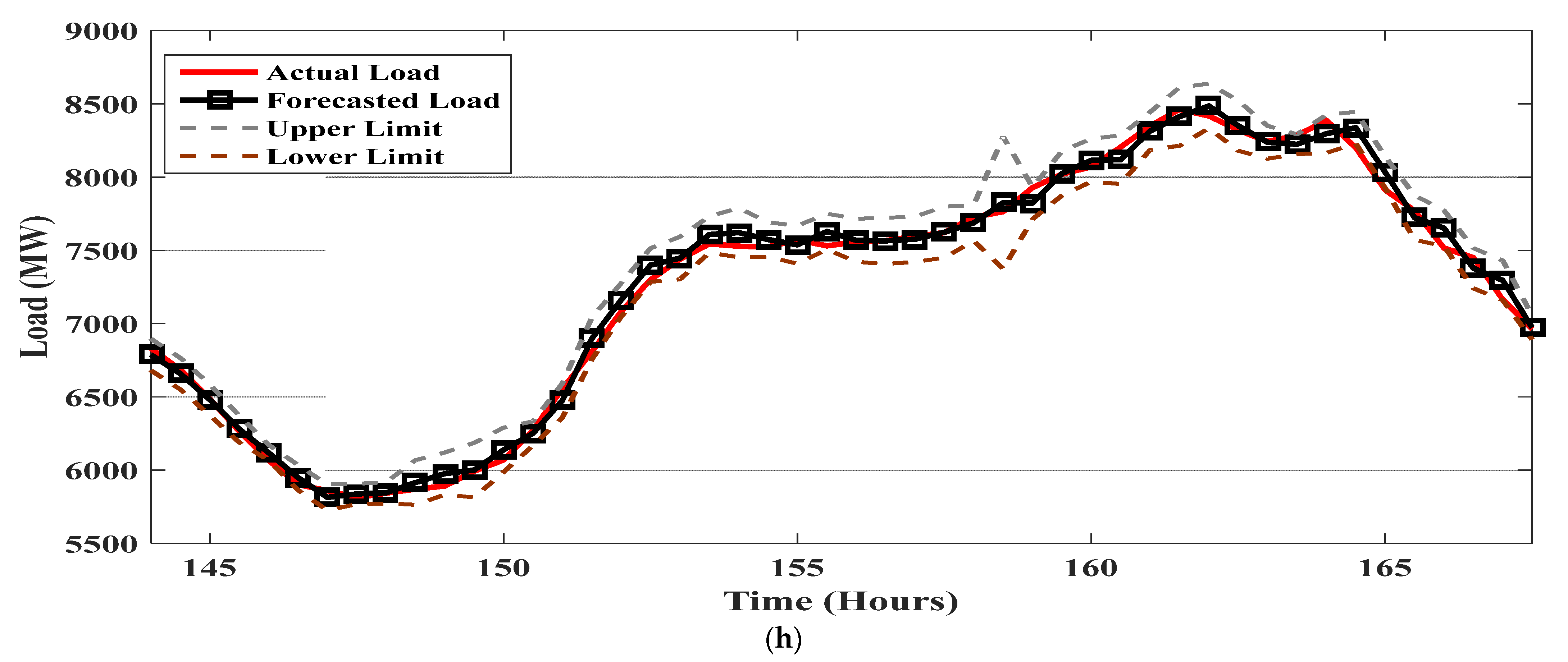
  • Application of confidence interval to fix the margins of error in the forecasted load;
  • Drawing certain insights on the number as well as type of features that affect the load in different seasons;
  • Comparing the performance of the proposed forecaster (with FS and WoFS) to the performance of forecasters based on J48 and Bagging.
The remaining sections of the paper are structured as follows. The methodology adopted for comparison of forecasts with FS and WoFS is discussed in Section 2. Section 3 explains the STLF using the M5P forecaster. Section 4 elucidates the methodology used for input feature selection using the novel HFS algorithm. The results and performance of the proposed methodology are presented in Section 5. Conclusions and remarks concerning findings are provided in Section 6.

2. Methodology Adopted for Comparison of Forecasts with FS and WoFS

In this work, STLF with FS and WoFS for next day was considered. For STLF, the proposed HFS algorithm is based on EGA and the random forest method. STLF was implemented using the concept of a similar week for each day and for all seasons on a half-hourly basis. STLF was performed using the M5P forecaster employing the full input feature set as well as with the selected (reduced) input feature set. The forecast accuracy was compared between using the full input feature set and using the reduced input feature set, validating the utility of STLF with a reduced input feature set.
The performance results obtained from M5P (with FS and WoFS) were also compared with the forecasts based on J48 and Bagging.
Accordingly, to ascertain the superiority of FS, the methodology adopted meant for comparison of forecasts with FS and WoFS is shown in Figure 1.

3. STLF Using M5P Forecaster Model

M5P is an ML algorithm which is a modified version of the M5 tree algorithm [39] and is used for both classification as well as regression problems. This modification allows it to deal with attribute missing values and enumerated attributes. M5P gives better results with longer data series as input since it is more sensitive to data splitting. The M5 tree was developed for the prediction of continuous variables and it serves as a flexible prediction tool since the construction of the tree is based on a multivariate linear model [40]. Generally, the M5 tree is a three-step process, i.e., construction of tree using input data, tree pruning and tree smoothing, whereas the M5P model consists of five important steps. M5P is a binary regression tree that stores a linear regression model at every leaf (last node), which predicts the class value of incoming instances. It uses the splitting criterion for the best split of a portion of training data that reaches any node. In the M5P tree, the standard deviation of the portion is used as a measure of error at that node. The tree of the M5P model is shown in Figure 2. The five steps of the M5P forecaster model are elaborated as follows:
Step 1:For the algorithm to maximize the standard deviation reduction (SDR), the input data (enumerated attributes) are taken and converted to binary variables using expression (1).
SDR = σ ( Cs ) k | Cs k | | Cs | × σ ( Cs k )
where Cs is the data set of STLF, Cs k is the kth subset of STLF, σ ( Cs k ) is the standard deviation of the kth subset of STLF as a measure of error and σ ( Cs ) is the standard deviation of Cs .
Step 2: The tree is constructed with these binary variables. Overfitting increases as the size of the tree grows. Here, the data overfitting problem will be overcome.
Step 3: To reduce the problem of overfitting, there is a pruning process and discontinuities are compensated.
Step 4: The tree smoothing process is included to balance sharp discontinuities that take place between linear adjacent models at the end nodes (leaf) of the pruned tree.
Step 5: Output is produced as a tree model.

4. Input Feature Selection Using the Proposed HFS Algorithm

Based on Darwin’s theory of natural evolution and the genetics of survival of the fittest, the genetic algorithm (GA) is one of the elite and heuristic search techniques and is used to produce useful solutions to optimization problems. The assumption of the relationships between characteristics involved was not considered in this approach when searching the space for FS. GA can easily encode decisions as Boolean value sequences, permitting the feature space to be explored by retaining the choices that support the classification task. Due to its inherent randomness, it also prevents local optimums concurrently. To solve optimization problems, it also makes use of operators inspired by natural evolution viz. selection, mutation and crossover.
Regression trees are traditionally used to predict data provided by the values of the function. A novel HFS algorithm based on EGA and the random forest method was used in this work. In EGA, 20% of the elite population is transferred to the next generation, through which the next generation has a feature set population whose classification accuracy is no less than that of the previous generation. The stratified 10-fold cross-validation (10-FCV) classification accuracy of a given dataset is used as the fitness function. In the present problem, strings of 1 s and 0 s are taken as chromosome segments, with 0 signifying that the feature corresponding to the index is not selected and 1 signifying that the relevant feature is selected. The length of the string is equal to the number of features in the dataset. The stratified 10-FCV classification accuracy (which is measured by means of the WEKA data mining workbench), using a random forest classifier, is all the fitness function computation. Classification accuracy refers to an approximation of the correctly identified number of instances. Roulette wheel selection is used here, and then a single-site crossover is carried out with a probability of 0.7 at each step. Mutation also occurs with a probability of 0.005. In addition, 20% of the elite population is transferred to the next generation. The best collection of features selected through final combination or encoding of chromosomes is given for STLF. The flowchart of the proposed novel HFS algorithm is depicted in Figure 3.

5. Results and Discussions

For STLF, half-hourly historical load data for New South Wales, Australia, and weather data for Sydney for the period January 2014 to June 2016 were obtained from the Australian Energy Market Operator (AEMO) and weatherzone.com.au, respectively. Humidity, wind speed and temperature have been considered as weather data. The EGA algorithm is run in MATLAB, while the formation of optimal tree is carried out in WEKA software. WEKA software is interfaced with MATLAB to perform all regression tree calculations. Final forecasting is carried out using MATLAB. Table 2 lists the input variables affecting the half-hourly STLF.
Each data set for STLF has 25 input features and a total of 2016 data sets were used in a training set to forecast the electricity load. The results derived from the proposed study are explained in two parts—the importance of FS is discussed in the first part and the various performance measures to compute the forecast accuracy is presented in the second part. The input features set for FS, which affects STLF, are taken from Table 2 and forecasting is carried out on the concept of similar week. Data sets were considered on the basis of similar weeks. Each data set consists of six weeks, i.e., for a given week to be forecasted, the preceding and successive two weeks along with the same week corresponding to the previous year were considered, while one preceding week of the same year was also included. For instance, if the input FS or forecasting of the electricity load is to be done for the week of 15–21 January 2016, the training set would consist of the data corresponding to 8–14 January 2016, 15–21 January 2015, 8–14 January 2015, 1–7 January 2015, 22–28 January 2015 and 29 January–4 February 2015. To obtain the FS, the accuracy of the data set for the proposed HFS was computed using 10-FCV. All the data were tested with this algorithm at least once. Thus, FS is the only algorithm that can be used to perform feature analysis.
Table 3 shows the number of times a particular input feature was selected out of the total 36 times for which the input FS was made.
It is clear from Table 3 that the input feature load of the present-day (Ld1), (Ld2) and (Ld3) are significant variables and are selected 36, 29 and 22 times, respectively. The variable wind speed of the present day (Ws3) is selected more often than the previous day. Moreover, the input feature temperature of the present day (Tem3) is often selected as compared to the previous day of the present day. On the other hand, the humidity of the present day (Hy2) was found to be selected more often than the previous day. The input feature hour type (HTo) is selected in all the runs, i.e., 36 times.
The effects of features can also be analyzed according to seasons. Table 4 shows the season-wise significance of different features. From Table 4, it can be seen that Ld2, Ld1, Ws2, etc., are the features that assume more significance during the winter season. Ld2, Ls3, etc., are the features that assume higher priority during the spring season. Ld2, Tem3, etc., are the features that assume higher priority during the summer season. The input feature load of the present day Ld1 and hour type HTo seems to be a feature, regardless of the season. These analyses point out the relative significance of the feature in terms of seasonal variations.
Performance measures viz. mean absolute percentage error (MAPE), error variance (EV), root mean square error (RMSE) and mean absolute error (MAE) were used to assess the numerical accuracy of the load forecasting [41].
The average error of each method was calculated week-wise for all seasons. Table 5 depicts the comparison between the M5P + FS approach and five other approaches (J48, Bagging, J48 + FS, Bagging + FS, and M5P) in terms of various performance measures viz. MAPE, MAE, EV and RMSE. The overall average performance for each method is also summarized in the last column. The results show that the M5P + FS method performs better than the rest of the methods used for comparison.
The error of electricity load is evaluated for the four prior weeks and at regular intervals of half an hour to calculate the confidence interval for one day. Afterward, half-hourly standard deviations (∆) and (2∆) were computed for 95% confidence interval. The lower and upper limits are computed as follows:
Lower Limit = Forecast value − 2∆
Upper Limit = Forecast value + 2∆
Results corresponding to the proposed methodology for the winter, spring and summer for the Australian electricity market are shown in Figure 4, Figure 5 and Figure 6, respectively. Table 5 clearly shows that the proposed method (M5P + FS) performs better than other methods in terms of all performance measures in all seasons.
Table 6 shows the percentage improvement attained with the proposed method (M5P + FS) over the other approaches. It is noted that the proposed methodology resulted in a 59.51% improvement compared to J48. It is also worth noting that M5P + FS has enhanced forecast accuracy over all considered methods.
The daily MAPEs corresponding to M5P and M5P + FS are calculated in Table 7. The graphical representations of daily MAPE for the all seasons are depicted in Figure 7, Figure 8 and Figure 9. These results show that the performance of M5P+ FS is completely superior to the performance of M5P.
To validate the proposed model, the MAPE values presented in this work were compared with those reported in [42] using another method and considering similar data sets. This will certainly help readers to enhance their understanding of this work since MAPE is one of the most commonly used key performance indicators to measure forecast accuracy (i.e., the lower the MAPE, the higher the forecast accuracy). The results listed in Table 8 clearly show that the proposed method performed better than previously reported methods.

6. Conclusions

In this paper, a day-ahead STLF employing M5P and a novel HFS approach based on EGA and the random forest method was presented. STLF was implemented for a whole year (in a week-wise manner for each day and for all seasons) with FS and WoFS. Performance measures such as MAPE, MAE, EV and RMSE were computed season-wise, week-wise and day-wise. The proposed methodology (M5P + FS) consists of two stages; i.e., in the first stage, FS is performed using the HFS algorithm and then in the second stage, forecasting is carried out by forecasters (M5P, Bagging and J48). For STLF with FS and WoFS, the results obtained with the M5P forecaster model were been compared with those obtained with J48 and Bagging. It is evident from the simulation results that the FS approach provides better short-term load forecasts over the WoFS approach and M5P outperforms J48 and Bagging. It is also evident that M5P + FS can offer improved accuracy (MAPE) in the range of 34.65 (for Bagging) to 59.51 (for J48).

Author Contributions

Software, methodology, conceptualization, investigation, validation and data curation, A.S.P. and A.K.S.; formal analysis, writing—original draft, supervision and visualization, A.K.S., V.K., S.M.T., A.S.P. and R.M.E.; editing and writing—review S.M.T., A.K.S., D.K., S.G. and M.A.H. All authors have read and agreed to the published version of the manuscript.

Funding

This research received no external funding.

Data Availability Statement

The half hourly historical load data of New South Wales, Australia taken from Australian Energy Market Operator (AEMO)) and weather data of Sydney City (www.weatherzone.com.au, accessed on 14 December 2022) has been taken for the STLF.

Conflicts of Interest

The authors declare no conflict of interest.

Abbreviations

AEMOAustralian Energy Market Operator
ANNArtificial Neural Network
ARMAAuto Regressive Moving Average
CLCClosed Loop Clustering
CNNConvolutional Neural Network
DEDifferential Evolution
DRBFNNsDecay Radial-Basis Function Neural Networks
DRMDynamic Regression Model
ELMExtreme Learning Machine
EGAElitist Genetic Algorithm
EVError Variance
FCVFold Cross-Validation
FSFeature Selection
GAGenetic Algorithm
GENCOsGeneration Companies
HFSHybrid Feature Selection
HWTHolt Winters Taylor
IEMDImproved Empirical Mode Decomposition
IFSIn Function Systems
LMLevenberg Marquardt
LRLasso Regression
LSTMLong Short Term Memory
MABCMulti-Species Artificial Bee Colony
MAE Mean Absolute Error
MAPE Mean Absolute Percentage Error
MLPMulti Layer Perception
MLMachine Learning
NSWNew South Wales
RMSERoot-Mean Square Error
SDRStandard Deviation Reduction
STLFShort-Term Load Forecasting
SVDSingular Value Decomposition
SVR Support Vector Regression
SVMSupport Vector Machine
WoFSWithout Features Selection
WTWavelet Transform
10-FCV10 Fold Cross Validation

References

  1. Muratori, M.; Rizzoni, G. Residential demand response: Dynamic energy management and time-varying electricity pricing. IEEE Trans. Power Syst. 2016, 31, 1108–1117. [Google Scholar] [CrossRef]
  2. Bunn, D.W. Forecasting loads and prices in competitive powermarkets. Proc. IEEE 2000, 88, 163–169. [Google Scholar] [CrossRef]
  3. Voronin, S.; Partanen, J. A Hybrid electricity price forecasting model for the Finnish electricity spot market. In Proceedings of the 32st Annual International Symposium on Forecasting, Boston, MA, USA, 24–27 June 2012. [Google Scholar]
  4. Yun, Z.; Quan, Z.; Caixin, S.; Shaolan, L.; Yuming, L.; Yang, S. RBF neural network and ANFIS-based short-term load forecasting approach in real-time price environment. IEEE Trans. Power Syst. 2008, 23, 853–858. [Google Scholar]
  5. Mund, C.; Rathore, S.K.; Sahoo, R.K. A review of solar air collectors about various modifications for performance enhancement. Sol. Energy 2021, 228, 140–167. [Google Scholar] [CrossRef]
  6. Sobhani, M.; Campbell, A.; Sangamwar, S.; Li, C.; Hong, T. Combining weather stations for electric load forecasting. Energies 2019, 12, 1510. [Google Scholar] [CrossRef] [Green Version]
  7. Melissa, D.; Binita, K.; Colin, C.I. Extreme Weather and Climate Vulnerabilities of the Electric Grid: A Summary of Environmental Sensitivity Quantification Methods; No. ORNL/TM-2019/1252; Oak Ridge National Lab. (ORNL): Oak Ridge, TN, USA, 2019. [Google Scholar]
  8. Dar-Mousa, R.N.; Makhamreh, Z. Analysis of the pattern of energy consumptions and its impact on urban environmental sustainability in Jordan: Amman City as a case study. Energy Sustain. Soc. 2019, 9, 15. [Google Scholar] [CrossRef] [Green Version]
  9. Tso, G.K.; Yau, K.K. Predicting electricity energy consumption: A comparison of regression analysis, decision tree and neural networks. Energy 2007, 32, 1761–1768. [Google Scholar] [CrossRef]
  10. Alghandoor, A.; Phelan, P.; Villalobos, R.; Phelan, B. US manufacturing aggregate energy intensity decomposition: The application of multivariate regression analysis. Int. J. Energy Res. 2008, 32, 91–106. [Google Scholar] [CrossRef]
  11. Zaza, F.; Paoletti, C.; LoPresti, R.; Simonetti, E.; Pasquali, M. Multiple regression analysis of hydrogen sulphide poisoning in molten carbonate fuel cells used for waste-to-energy conversions. Int. J. Hydrogen Energy 2011, 36, 8119–8125. [Google Scholar] [CrossRef]
  12. Kumar, U.; Jain, V. Time series models (Grey-Markov, Grey Model with rolling mechanism and singular spectrum analysis) to forecast energy consumption in India. Energy 2010, 35, 1709–1716. [Google Scholar] [CrossRef]
  13. Rumbayan, M.; Abudureyimu, A.; Nagasaka, K. Mapping of solar energy potential in Indonesia using artificial neural network and geographical information system. Renew. Sustain. Energy Rev. 2012, 16, 1437–1449. [Google Scholar] [CrossRef]
  14. Matallanas, E.; Castillo-Cagigal, M.; Gutiérrez, A.; Monasterio-Huelin, F.; Caamaño-Martín, E.; Masa, D.; Jiménez-Leube, J. Neural network controller for active demand-side management with PV energy in the residential sector. Appl. Energy 2012, 91, 90–97. [Google Scholar] [CrossRef] [Green Version]
  15. Cheong, C.W. Parametric and non-parametric approaches in evaluating martingale hypothesis of energy spot markets. Math. Comput. Model. 2011, 54, 1499–1509. [Google Scholar] [CrossRef]
  16. Wesseh, P.K., Jr.; Zoumara, B. Causal independence between energy consumption and economic growth in Liberia: Evidence from a non-parametric bootstrapped causality test. Energy Policy 2012, 50, 518–527. [Google Scholar] [CrossRef]
  17. Grzegorz, D. Pattern-based local linear regression models for short-term load forecasting. Electr. Power Syst. Res. 2016, 130, 139–147. [Google Scholar]
  18. Cecati, C.; Kolbusz, J.; Rozycki, P.; Siano, P.; Wilamowski, B.M. A Novel RBF Training Algorithm for Short-Term Electric Load Forecasting and Comparative Studies. IEEE Trans. Ind. Electron. 2015, 62, 6519–6529. [Google Scholar] [CrossRef]
  19. Zhai, M.-Y. A new method for short-term load forecasting based on fractal interpretation and wavelet analysis. Int. J. Electr. Power Energy Syst. 2015, 69, 241–245. [Google Scholar] [CrossRef]
  20. Arora, S.; Taylor, J.W. Short-Term Forecasting of Anomalous Load Using Rule-Based Triple Seasonal Methods. IEEE Trans. Power Syst. 2013, 28, 3235–3242. [Google Scholar] [CrossRef] [Green Version]
  21. Zeng, P.; Jin, M.; Elahe, M.F. Short-Term Power Load Forecasting Based on Cross Multi-Model and Second Decision Mechanism. IEEE Access 2020, 8, 184061–184072. [Google Scholar] [CrossRef]
  22. Nose-Filho, K.; Lotufo, A.D.P.; Minussi, C.R. Short-Term Multinodal Load Forecasting Using a Modified General Regression Neural Network. IEEE Trans. Power Deliv. 2011, 26, 2862–2869. [Google Scholar] [CrossRef]
  23. Zhang, C.; Li, R. A Novel Closed-Loop Clustering Algorithm for Hierarchical Load Forecasting. IEEE Trans. Smart Grid 2021, 12, 432–441. [Google Scholar] [CrossRef]
  24. Rafi, S.H.; Nahid-Al-Masood; Deeba, S.R.; Hossain, E. A Short-Term Load Forecasting Method Using Integrated CNN and LSTM Network. IEEE Access 2021, 9, 32436–32448. [Google Scholar] [CrossRef]
  25. Song, L.; Peng, W.; Lalit, G. Short-term load forecasting by wavelet transform and evolutionary extreme learning machine. Electr. Power Syst. Res. 2015, 122, 96–103. [Google Scholar]
  26. Kouhi, S.; Keynia, F.; Ravadanegh, S.N. A new short-term load forecast method based on neuro-evolutionary algorithm and chaotic feature selection. Int. J. Electr. Power Energy Syst. 2014, 62, 862–867. [Google Scholar] [CrossRef]
  27. Ungureanu, S.; Topa, V.; Cziker, A.C. Analysis for Non-Residential Short-Term Load Forecasting Using Machine Learning and Statistical Methods with Financial Impact on the Power Market. Energies 2021, 14, 6966. [Google Scholar] [CrossRef]
  28. Luo, J.; Hong, T.; Yue, M. Real-time anomaly detection for very short-term load forecasting. J. Mod. Power Syst. Clean Energy 2018, 6, 235–243. [Google Scholar] [CrossRef] [Green Version]
  29. Jiao, R.; Zhang, T.; Jiang, Y.; He, H. Short-term non-residential load forecasting based on multiple sequences LSTM recurrent neural network. IEEE Access 2018, 6, 59438–59448. [Google Scholar] [CrossRef]
  30. Haq, M.R.; Ni, Z. A new hybrid model for short-term electricity load forecasting. IEEE Access 2019, 7, 125413–125423. [Google Scholar] [CrossRef]
  31. Deng, Z.; Wang, B.; Xu, Y.; Xu, T.; Liu, C.; Zhu, Z. Multi-scale convolutional neural network with time-cognition for multi-step short-term load forecasting. IEEE Access 2019, 7, 88058–88071. [Google Scholar] [CrossRef]
  32. Hong, Y.; Zhou, Y.; Li, Q.; Xu, W.; Zheng, X. A deep learning method for short-term residential load forecasting in smart grid. IEEE Access 2020, 8, 55785–55797. [Google Scholar] [CrossRef]
  33. Ahmad, W.; Ayub, N.; Ali, T.; Irfan, M.; Awais, M.; Shiraz, M.; Glowacz, A. Towards short term electricity load forecasting using improved support vector machine and extreme learning machine. Energies 2020, 13, 2907. [Google Scholar] [CrossRef]
  34. Pei, S.; Qin, H.; Yao, L.; Liu, Y.; Wang, C.; Zhou, J. Multi-step ahead short-term load forecasting using hybrid feature selection and improved long short-term memory network. Energies 2020, 13, 4121. [Google Scholar] [CrossRef]
  35. Xuan, Y.; Si, W.; Zhu, J.; Sun, Z.; Zhao, J.; Xu, M.; Xu, S. Multi-model fusion short-term load forecasting based on random forest feature selection and hybrid neural network. IEEE Access 2021, 9, 69002–69009. [Google Scholar] [CrossRef]
  36. Ijaz, K.; Hussain, Z.; Ahmad, J.; Ali, S.F.; Adnan, M.; Khosa, I. A Novel Temporal Feature Selection Based LSTM Model for Electrical Short-Term Load Forecasting. IEEE Access 2022, 10, 82596–82613. [Google Scholar] [CrossRef]
  37. Zhang, S.; Zhang, N.; Zhang, Z.; Chen, Y. Electric Power Load Forecasting Method Based on a Support Vector Machine Optimized by the Improved Seagull Optimization Algorithm. Energies 2022, 15, 9197. [Google Scholar] [CrossRef]
  38. Liu, M.; Qin, H.; Cao, R.; Deng, S. Short-Term Load Forecasting Based on Improved TCN and DenseNet. IEEE Access 2022, 10, 115945–115957. [Google Scholar] [CrossRef]
  39. Yi, H.S.; Lee, B.; Park, S.; Kwak, K.C.; An, K.G. Prediction of short-term algal bloom using the M5P model-tree and extreme learning machine. Environ. Eng. Res. 2019, 24, 404–411. [Google Scholar] [CrossRef]
  40. Kisi, O.; Shiri, J.; Demir, V. Hydrological time series forecasting using three different heuristic regression techniques. In Handbook of Neural Computation; Academic Press: Cambridge, MA, USA, 2017; pp. 45–65. [Google Scholar]
  41. Srivastava, A.K.; Pandey, A.S.; Elavarasan, R.M.; Subramaniam, U.; Mekhilef, S.; Mihet-Popa, L. A Novel Hybrid Feature Selection Method for Day-Ahead Electricity Price Forecasting. Energies 2021, 14, 8455. [Google Scholar] [CrossRef]
  42. Dudek, G. A Comprehensive Study of Random Forest for Short-Term Load Forecasting. Energies 2022, 15, 7547. [Google Scholar] [CrossRef]
Figure 1. Methodology adopted for comparison of forecasts with FS and WoFS.
Energies 16 00867 g001
Figure 2. M5P Tree.
Figure 2. M5P Tree.
Energies 16 00867 g002
Figure 3. Flow chart for feature selection using the proposed novel hybrid algorithm.
Energies 16 00867 g003
Figure 4. Forecasting in winter 1–7 August 2015 with M5P +FS, (a) entire week, (bh) daily forecast.
Energies 16 00867 g004aEnergies 16 00867 g004bEnergies 16 00867 g004c
Figure 5. Forecasting in spring 1–7 September 2015 with M5P + FS, (a) entire week, (bh) daily forecast.
Energies 16 00867 g005aEnergies 16 00867 g005bEnergies 16 00867 g005c
Figure 6. Forecasting in summer 1–7 Feb. 2016 with M5P + FS, (a) entire week, (bh) daily forecast.
Energies 16 00867 g006aEnergies 16 00867 g006bEnergies 16 00867 g006cEnergies 16 00867 g006d
Figure 7. Representation of daily MAPE for winter season corresponding to M5P and M5P + FS.
Energies 16 00867 g007
Figure 8. Representation of daily MAPE for spring season corresponding to M5P and M5P + FS.
Energies 16 00867 g008
Figure 9. Representation of daily MAPE for summer season corresponding to M5P and M5P + FS.
Energies 16 00867 g009
Table 1. Review of several past research studies on STLF.
Sr. No.YearAuthor [Ref.]Methodology UsedFeature SelectionPerforemnce Measure
MAPEMAERMSEEV
1.2018Luo et al. [28]Dynamic Regression Model (DRM)-based detection methodNoXXX
2.2018Jiao et al. [29]Multiple Sequence LSTM Recurrent Neural NetworkNoX
3.2019Haq et al. [30] T-Copula-IEMD-DBN MethodNoXX
4.2019Deng et al. [31]TCMS-CNN AlgorithmYesX
5.2020Hong et al. [32]Iterative Resblocks-Based Deep Neural Network (IRBDNN)NoX
6.2020Ahmad et al. [33]SVM-GS, ELM-GAYesX
7.2020Pei et al. [34]ILSTM network YesX
8.2021Rafi et al. [24]CNN-LSTM-based hybrid NetworkYes
9.2021Ungureanu et al. [27]LSTM, LSTMed, GRU, CNN-LSTMYesX
10.2021Xuan et al. [35]CNN-BiGRU AlgorithmYesXX
11.2022Ijaz et al. [36]Artificial Neural Network (ANN) layer and LSTMYesX
12.2022Zhang et al. [37]Improved Seagull Optimization Algorithm and SVM (ISOA-SVM) MethodNoX
13.2022Liu et al. [38]DenseNet-iTCN) Yes
Table 2. Input features affecting half-hourly STLF.
Class of Input FeatureTiming of Input FeatureName of Input Feature
Load (Ld)Ld(K-00.30)Ld1
Ld(K-01:00)Ld2
Ld(K-01:30)Ld3
Ld(K-24:00)Ld4
Ld(K-23:30)Ld5
Ld(K-23:00)Ld6
Wind speed (Ws)Ws(K-00.30)Ws1
Ws(K-01:00)Ws2
Ws(K-01:30)Ws3
Ws(K-24:00)Ws4
Ws(K-23:30)Ws5
Ws(K-23:00)Ws6
Temperature (Tem)Tem(K-00.30)Tem1
Tem(K-01:00)Tem2
Tem(K-01:30)Tem3
Tem(K-24:00)Tem4
Tem(K-23:30)Tem5
Tem(K-23:00)Tem6
Humidity (Hy)Hy(K-00.30)Hy1
Hy(K-01:00)Hy2
Hy(K-01:30)Hy3
Hy(K-24:00)Hy4
Hy(K-23:30)Hy5
Hy(K-23:00)Hy6
Hour timing (HTo)HTo(K-00.00)HTo
Table 3. Input feature selected (year-wise) for STLF.
Name of Input FeatureNumber of Times Input Feature SelectedName of Input FeatureNumber of Times Input Feature Selected
Ld6 17Tem611
Ld5 12Tem508
Ld412Tem412
Ld322Tem318
Ld229Tem212
Ld136Tem113
Ws602Hy607
Ws507Hy510
Ws409Hy412
Ws312Hy312
Ws211Hy214
Ws107Hy112
HTo36
Table 4. Input feature is selected (season-wise) for STLF.
Name of Input FeatureSummerWinterSpring
Ld6060605
Ld5030306
Ld4030306
Ld3060709
Ld2090911
Ld1121212
Ws6000101
Ws5030400
Ws4020502
Ws3020604
Ws2030701
Ws1020203
Tem6030305
Tem5020501
Tem4040602
Tem3080604
Tem2020505
Tem1060205
Hy6010402
Hy5030205
Hy4050403
Hy3040503
Hy2060503
Hy1020604
HTo121212
Table 5. Performance of proposed methodology in terms of various performance measures.
Sr. No.MethodologyName of Performance MeasuresSeasonMean
Winter (1–7 August 2015)Spring (1–7 September 2015)Summer (1–7 February 2016)
1J48MAPE1.661.821.421.63
J48 + FS1.371.530.951.28
Bagging1.210.980.831.01
Bagging + FS1.160.930.800.96
M5P1.070.990.640.90
M5P + FS0.670.700.610.66
2J48MAE147.39138.43108.40131.41
J48 + FS120.43114.0573.79102.76
Bagging106.5178.2864.0582.95
Bagging + FS102.4374.5262.0279.66
M5P93.7380.1549.5074.46
M5P + FS56.5455.4247.7653.24
3J48RMSE215.63221.77140.64192.68
J48 + FS190.14164.9595.13150.07
Bagging151.66108.7281.76114.05
Bagging + FS147.97100.7578.41109.04
M5P131.17107.0663.91100.71
M5P + FS73.0073.7560.3369.03
4J48EV0.000330.000550.000130.00034
J48 + FS0.000290.000260.000060.00020
Bagging0.000160.000090.000040.00010
Bagging + FS0.000150.000070.000040.00009
M5P0.000110.000080.000030.00007
M5P + FS0.000030.000040.000020.00003
Table 6. Improvement of different performance measures using M5P + FS compared to other approaches for STLF.
Sr. No.MethodologyMean MAPEPercentage Improvement (%)
1.M5P +FS0.66-
2.J481.6359.51
3.J48 + FS1.2848.44
4.Bagging1.0134.65
5.Bagging + FS0.9631.25
6.M5P0.9026.67
Sr. No.MethodologyMean MAEPercentage Improvement (%)
1.M5P +FS53.24-
2.J48131.4159.48
3.J48 + FS102.7648.19
4.Bagging82.9535.81
5.Bagging + FS79.6633.16
6.M5P74.4628.50
Sr. No.MethodologyMean RMSEPercentage Improvement (%)
1.M5P +FS69.03-
2.J48192.6864.18
3.J48 + FS150.0754.01
4.Bagging114.0539.48
5.Bagging + FS109.0436.70
6.M5P100.7131.46
Table 7. Daily MAPE for all seasons corresponding to M5P and M5P + FS.
Sr. No.(1–7 Aug 2015) Winter(1–7 Sep 2015) Spring(1–7 Feb 2016) Summer
M5PM5P + FSM5PM5P + FSM5PM5P + FS
10.950.691.120.530.660.63
21.600.920.980.540.610.54
31.260.941.000.660.480.49
40.920.600.920.600.580.63
51.090.580.800.710.710.65
60.900.480.830.820.650.61
70.790.461.261.070.750.73
5.251.070.670.990.700.64
Table 8. Validation of proposed method.
Sr. No.DurationMethodologyMAPE
11–7 December 2015Random Forest [42]1.02
2Proposed Algorithm (M5P + FS)0.70
Disclaimer/Publisher’s Note: The statements, opinions and data contained in all publications are solely those of the individual author(s) and contributor(s) and not of MDPI and/or the editor(s). MDPI and/or the editor(s) disclaim responsibility for any injury to people or property resulting from any ideas, methods, instructions or products referred to in the content.

