Experimental Study of an Inverter Control for Reactive Power Compensation in a Grid-Connected Solar Photovoltaic System Using Sliding Mode Control

Abstract

In photovoltaic (PV) systems, inverters have an essential role in providing an energy supply to meet the demand with power quality. Inverters inject energy into the grid considering that a renewable source is available; however, during intermittent periods or in the absence of power generation, the inverter remains inactive, which decreases the performance of the PV system. One way to increase the operation of inverters is to operate them as Volt-Amps Reactive (VAR) compensators to generate reactive power in the absence of renewable sources. The paper presents the development of a control scheme that allows the PV system’s inverter to improve the power factor in the electrical system with or without PV power generation. The proposed control is based on using a sliding mode controller (SMC) current control loop and PI-based voltage control loop. The control scheme is developed in MATLAB/SIMULINK, and for real evaluation, a PV prototype is implemented. The control strategy efficiency is confirmed by the obtained results. The control scheme increases the practical utility of PV systems. Additionally, it improves the power factor in all cases during the injection of active power to the grid operating under intermittent conditions and/or in the absence of power generation.

1. Introduction

Currently, the most popular renewable energy source in the world is solar PV energy due to technological advances and lower prices [1]. Globally, installations of rooftop photovoltaic systems have increased. Typical single-stage PV systems comprise a PV array and an inverter as a DC-AC power conversion station in a grid-connected system. Inverters play a key role in improving the efficiency and the power quality injected into the grid in PV-based power generation. PV systems do not perform well during cloudy days or nights, and this intermittent behavior affects the availability, reliability, and quality of the distributed grid [2,3]. Further during the operation of a PV system, the active power supplied to the grid is reduced due to the active and reactive power used to supply the power demanded by the connected load. According to the power triangle, the reduction in active power results in an increased power factor (PF) angle; therefore, it can reduce the PF below the acceptable limit [4]. With the use of control theory, it is possible to obtain the maximum utilization factor from renewable sources (e.g., the sun). It is possible to manage the energy generated by the system and ensure the injection of energy that is free of disturbances into the grid with the inverter control schemes.

One way to take maximum benefits from PV systems is to increase the functions performed by the inverter because it accomplishes multiple functions involving both reactive and real power control besides its primary task of converting [5,6]. When the power generation is available, the inverter operates as a static compensator (STATCOM) device to generate reactive power to meet the demand generated from the loads; additionally, it injects active power into the grid. When a renewable source is not available, the inverter only serves as a reactive power (VAR) compensator and provides an improvement in PF.

Consequently, the importance of reactive power control laws applied to PV inverters arises from the fact that common loads are especially non-linear [7]; these loads deteriorate the PF and create power quality problems that may affect other loads connected at the same point of common coupling (PCC) [8,9]. Proper reactive power compensation can significantly improve the system reliability, given that a unity PF is achieved and the losses in the electric lines are reduced [10,11]. Therefore, this may attenuate the voltage regulation problems and maximize the power transmission capability by reducing the transmission loss. Inverters operating as STATCOM devices have been reported, where the control strategy can open a new revenue-making opportunity for PV inverters to provide the STATCOM service cheaper [12]. That the inverter can perform multiple functions is associated mainly with the electronic controllers and control algorithms [13,14]. Accordingly, quality inverter controllers are required to generate power in PV systems, such as digital control circuits, microcontrollers or microcomputers, or digital signal processors (DSPs) [15].

Therefore, the development of control algorithms used in PV inverter controllers for sustainable renewable energy applications is inevitable because it contributes to generating clean energy without compromising the availability and reliability of the electricity supply [16]. The inverter control system has its aims to ensure that the variable output is controlled so it resembles and tracks the desired output.

The SMC is of interest because it is a particular class of variable-structure systems and is considered a fast and robust non-linear control technique suitable for regulating switched-controlled systems [17]. This control law is a time-varying state feedback algorithm, which changes at a high frequency from one continuous structure to another according to the current position of the state variables; the control aim is to make the output variable track the desired profile, that is, the output error variable tends to some small vicinity of zero after a transient of an acceptable duration [18]. Compared to other control schemes, SMC is easy to implement and highly robust and stable during the load and/or other parameters variations [19]. These features make the SMC scheme highly appropriate for dealing non-linear systems. Therefore, SMC is one of the widely used schemes adopted by the power industry for many applications such as electric drives and power converters [20,21,22]. Similarly, many studies have shown that the SMC-based control scheme provides shorter settling times and oscillating responses and less overshoot in a three-phase grid-coupled PV system [23].

However, for a real-time grid-coupled PV system, it is challenging to build an efficient SMC reactive power compensation scheme. This paper provides the design and real implementation of an SMC-based control of a PV system with PF improvement. It is essential to mention that the proposed work is established from work given in [24,25]. The proposed SMC seeks to enhance inverter performance and ensure PF compensation to create a more flexible SMC that protects against parameter variations and guarantees stability. The main contributions of this work are as follows:

• The grid-connected PV system supplies active power and compensates for the reactive power of the local non-linear load connected to the PCC.
• It is important to note that the control scheme allows the PV system to continue operating and improves the PF of non-linear loads connected in intermittent periods or in the total absence of power generation.
• The proposed scheme is confirmed by an SMC for current reference tracking and is PI-based to regulate the capacitor voltage for the inverter operation in the absence of power generation from a PV array.
• The system behavior verifies that the SMC technique is adequate and allows the inverter to improve the PF and decrease the total harmonic distortion (THD) value of the grid current injected into the grid by the PV system.

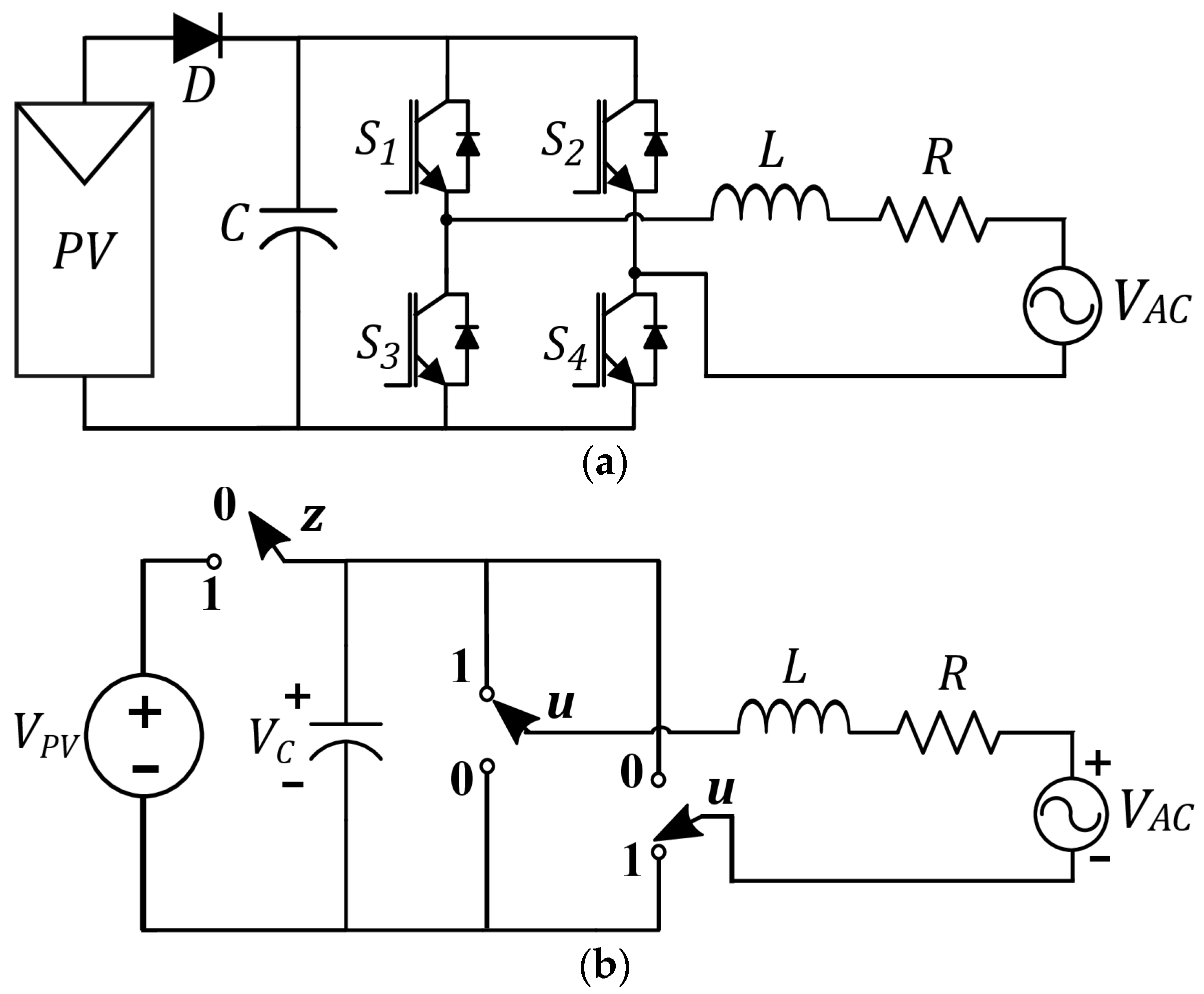
2. System Description

The equivalent circuit of the grid-connected PV system is described in Figure 1a; it is composed of a PV array with a capacitor (C) parallel connected by a diode (D) as the main switch. The capacitor is connected to the inverter power input. The inverter output is interconnected to the grid through the RL filter. The proposed electrical scheme without a DC converter has been extensively studied due to its non-linear behavior [24].

Two operation conditions determine the described system performance (Figure 1b); the state of the control variable z determines these states. When $z=1$, the power generation from the PV array is available, when $z=0$, there is no power generation. In the electric scheme, the operating conditions are determined by D, which is a natural switch for current flow. When there is power generation available, the PV array voltage (V_PV) is higher than the peak value of the grid voltage (V_AC). In this case, the capacitor operates as an energy storage and protection device against abrupt voltage changes. $z=1$ determines this condition.

Otherwise, when there is no power generation from the PV array, the voltage generated by the panels is less than the peak value of the grid voltage (V_PV < V_AC), the capacitor works as an energy source, allowing the system to continue operating, and $z=0$ determines this condition. The inverter converts the output DC voltage from the PV array to AC voltage for supplying the grid and operates independently of the availability or absence of power generation of the PV array. The inverter circuit comprises an H bridge formed by switches S₁, S₂, S₃, and S₄, and these devices commute according to a control strategy. The control variable u determines these state changes in its operation; this control signal is based on the error signal level to determine the specific control signals to feed the switching devices [24]. In its operation, the inverter takes the DC power generated from the PV array and generates an AC output interconnected to the grid through an RL filter; the filter cancels the signals generated by the high-frequency switching of S₁, S₂, S₃, and S₄. In Figure 1b, the complete system described based on the control variables involved is presented.

2.1. Operation with Power Generation

The operation condition is determined when the generation is available from the PV array and the following condition is accomplished: $V_{PV}>V_{AC}$. The control variable that determines the status of the diode is $z=1$. Figure 2 shows the cases obtained in the two states of the control signal u. In this case, $V_{C }=V_{PV}$, and its value could be omitted from the analysis. When the control signal $u=1$, in Figure 2a, the electrical circuit obtained is presented, and Figure 2b shows the electric circuit when the control signal $u=0$.

In summary, for the state $z=1$, the dynamics $i_L$ of the system are a function of the control, and variable $u$ is determined by (1). The detailed process is presented in [24].

$$L\frac{d{i}_L}{dt}=\left(2u-1\right) V_{PV}-i_{L}R-V_{AC}$$

(1)

2.2. Operation without Power Generation

When there is no generation by the panels and the condition $V_{PV}<V_{AC}$ is accomplished, this operating condition is active. In this case, $z=0$ is the control variable that determines the status of the diode.

Figure 3 shows both cases obtained with the two states of the control signal $u$. In this case, the panel is disconnected, leaving capacitor $C$ as the element that will exchange energy with the grid. As there is no PV array power generation, the capacitor does not generate active power; it only injects reactive power to compensate for the demand of the load. In Figure 3a the electrical circuit obtained when the control signal $u=1$ is presented, and in Figure 3b, the circuit obtained with a control signal $u=0$ is presented.

Finally, it is possible to obtain the dynamics of the system based on the two control variables involved ($z, u$). Therefore, the mathematical model of the complete system is determined by (2) and (3). The detailed process is presented in [24].

$$L\frac{d{i}_L}{dt}=\left(2u-1\right)\left[z{V}_{PV }+\left(1-z\right)V_C\right]-i_{L}R-V_{AC}$$

(2)

$$C\frac{d{V}_C}{dt}=\left(1-z\right)\left(1-2u\right) i_L$$

(3)

3. Control Scheme

The proposed scheme is shown in Figure 4 and is made up of the following sections:

-

The power source is a PV array; in parallel, a capacitor is connected through a power diode, which prevents the return of the electrical current from the grid current to the solar PV array. The capacitor is the virtual power source in periods when the panel is not inactive.

-

The inverter performs the DC-to-AC power conversion and produces controllable current output.

-

An inductive filter RL was placed between the inverter output and grid to cancel switching harmonics.

-

An inductive load, as a reference, is PCC-connected.

-

To obtain i_L, an active power estimator from the PV array and the voltage loop are used to maintain the capacitor voltage in the period of the absence of PV energy. The estimator information is obtained by the maximum power tracking algorithm (MPPT) of the PV array and guarantees the balance of power.

-

The DQ transform obtains the reactive power reference based on the signals that the PLL builds when synchronized with the main voltage. DQ is mentioned in Section 4.3.

-

The SMC loop is designed for current reference tracking through the generation of the control signal u. With the control signal and a proper PWM technique, the inverter produces output power with a low loss, a high efficiency, low distortion, a short computation time, and minimal harmonics [26]. With a proper modulation strategy, reactive power generation is achieved in inverter topologies without any alteration to the converter structure [27]. A Level-Shifted MultiCarrier PWM switching technique is employed to generate the desired output current. This modulation has been studied and widely used in multilevel inverter topologies for power quality improvement applications [28].

When the power generation PV array is not available from the PV array, the Proportional Integral (PI)-based voltage control loop guarantees that the $C$ works as a virtual power source for the inverter.

Figure 4. Control scheme.

Figure 4. Control scheme.

4. Control Theory

Two control loops integrate the proposed scheme. When the power generation from the PV panels is available, the current control loop based on SMC theory allows for the tracking of load current and also generates the compensation output current ($i_L^{*}$); therefore, the inverter is capable of compensating the reactive power and improving the PF of the current supplied by the grid-connected PV system. On the other hand, when the power generation is not available, in addition to the current control loop, the PI-based voltage control loop operation ensures the voltage level within the reference value of $C$ and the current flow in the PV system.

4.1. Voltage Control Loop

The voltage control loop proposed is based on a PI controller. The PI controller is selected because it offers a good dynamic response and zero steady-state errors in controlling a DC quantity [29]. The objective of the DC voltage regulation loop is to ensure output voltage regulation that is equal to the reference output voltage.

When the power generation from the PV panels is not available, the voltage control loop begins to work and guarantees that the $C$ works as a power source that allows the inverter to continue operating. In this operation mode, the control scheme has two control objectives. On the one hand, it tracks the $i_{Load}$ charge current to correct the PF; this is in addition to aiming to regulate the capacitor voltage ($V_C$) to a set value ($V_C^{*}$) that allows it to operate as a power source of the system. By meeting both control objectives, the PF correction by the inverter is guaranteed. The voltage control loop is a decoupled system considered, where the dynamics of the current control are fast enough to reach the desired current ($i_L^{*}$). Therefore, the expression of the dynamics system is reduced by (3). The equation can be described by:

$$f(i_L,u,z)=\frac{\left(1-z\right)\left(1-2u\right)i_L}{C}$$

(4)

Expression (4) can be seen as an input function in the dynamics of $V_C$; the transfer function, which relates the voltage of the capacitor to the input function, can be established:

$$\frac{V_C\left(S\right)}{F\left(S\right)}=\frac{1}{s}$$

(5)

The transfer function (5) represents a first-order subsystem that can be controlled through PI control; this is defined in the time domain by:

$$C_{PI}\left(S\right)=\left(K_p+\frac{K_i}{S}\right)\left[F\left(S\right)-V_C\left(S\right)\right]\left(1-z\right)$$

where $K_p$ is the proportional gain, and $K_i$ is the integral gain; when passing to the time domain, it is of the following form:

$$C_{PI}\left(t\right)=\left[K_p\left(V_c^{*}-V_C\right)+K_i{\displaystyle \int }\left(V_c^{*}-V_C\right)dt\right]\left(1-z\right)$$

(6)

where ($V_c^{*}-V_C$) represents the error between the desired value of the capacitor voltage ($V_c^{*}$) and that measured in the capacitor ($V_C$). The expression (6) controls based on the voltage error of the capacitor and its integral. The values of $K_p$ and $K_i$ gains determine the response of the system during the transient and stable state; therefore, keeps the output voltage as close as possible to the reference voltage.

4.2. Current Control Loop

The current control loop is SMC based, given that it has been widely used in power electronic equipment power converters being a natural field of application due to the abrupt changes in the state involved in electric circuits operation [30]. The SMC strategy composes an effective and high-frequency switching control for complex high-order non-linear systems with uncertainties. The system-controlled exhibits robustness properties to both internal parameter uncertainties and external disturbances [30,31].

In the basic principle of sliding mode, a sliding surface in state space is designed, and a control law to force the state trajectory of the system to move toward a predetermined surface in the time is selected; this is to maintain this surface with an appropriate switching logic [32]. The SMC controller is used to track load current ($i_{Load}$) and generate the control signal $u$ that determines the inverter operation. The inverter is able to inject the estimated current $i_L^{*}$ of compensation into the grid; this reference compensates reactive power load demanded and improves the PF. The current loop operation is not committed to the PV system modes of operation since the reactive power compensation is performed in the presence or absence of PV array power generation. The inverter is expected to produce an output current in phase with the utility voltage for obtaining a unity PF at all times.

The main steps to define the SMC control are:

Firstly, is to determine a sliding surface ($\sigma$) to enable the desired stable state asymptotic behavior where $e$ is the error respect time:

$$\sigma =\left(e,t\right)=0$$

(7)

With the equivalent control applied, the invariance condition is obtained:

$${\frac{d\sigma }{dt}|}_{\begin{array}{c}\sigma =0\\ u=u_{eq}\end{array}}=0$$

(8)

The existence of the equivalent control $u_{eq}$ represents the equivalent control solution and ensures the viability of a model on the sliding surface. In summary, the control law is obtained, and Lyapunov stability is guaranteed. With the steps described, the current inverter is chosen as a sliding surface based on the $e$ between the desired current ($i_L^{*}$) with the output measurement ($i_L$). The surface remains as:

$$\sigma =\left(e,t\right)=L\left(i_L-i_L^{*}\right)$$

(9)

The solution when $\sigma =\left(e,t\right)=0$ of (9) is given by:

$$i_L=i_L^{*}$$

(10)

$u_{eq}$ is obtained when the invariance condition is applied as shown in (8):

$$\frac{d\sigma \left(e,t\right)}{dt}=\frac{dL\left(i_L-i_L^{*}\right)}{dt}$$

$$L\frac{d{i}_L}{dt}-L\frac{d{i}_L^{*}}{dt}=0$$

(11)

The expression (2) is replaced in (11):

$$\left(2u-1\right)\left[z{V}_{PV}+\left(1-z\right)V_C\right]-i_{L}R-V_{AC}-L\frac{d{i}_L^{*}}{dt}=0$$

(12)

The expression (12) replaces the expression (10), obtaining:

$$u_{eq}=\frac{L\frac{d{i}_L^{*}}{dt}+i_L^{*}R+V_{AC}}{2\left[z V_{PV}+\left(1-z\right)V_C\right]}+\frac{1}{2}$$

(13)

To obtain the control law, an energy function that meets the stability criteria of Lyapunov is proposed. The function must meet two conditions:

$$V\left(\sigma \right)\ge 0$$

(14)

$$\frac{dV\left(\sigma \right)}{dt}\le 0$$

(15)

The energy function shown in (16) to guarantee condition (14) is proposed:

$$V\left(\sigma \right)=\frac{1}{2}{\sigma }^2$$

(16)

Applying the differential operator for condition (15) is obtained:

$$\frac{dV\left(\sigma \right)}{dt}=\sigma \frac{d\sigma }{dt}$$

$$\sigma \frac{d\sigma }{dt}=\left[L\left(i_L-i_L^{*}\right)\right]\left[L\frac{d{i}_L}{dt}-L\frac{d{i}_L^{*}}{dt}\right]$$

(17)

To guarantee compliance with this condition, the theory proposed by [33] is applied, which determines that the second Lyapunov condition must contain a term of the absolute value of the sliding surface. Therefore, the differential operator of condition (17) is proposed and has the form:

$$\frac{dV\left(\sigma \right)}{dt}=-\beta \left|\sigma \right|$$

(18)

Where β is a strictly positive value to guarantee compliance with this second Lyapunov condition. By equating expressions (17) and (18) the following expression is obtained:

$$L\frac{d{i}_L}{dt}-L\frac{d{i}_L^{*}}{dt}=-\beta \mathrm{sgn}\left(\sigma \right)$$

(19)

By reordering the terms, the control law is obtained:

$$u=\frac{L\frac{d{i}_L^{*}}{dt}+i_L^{*}R+V_{AC}-\beta \mathrm{sgn}\left(i_L-i_L^{*}\right)}{2\left[z V_{PV}+\left(1-z\right)V_C\right]}+\frac{1}{2}$$

(20)

According to [34], the control law obtained must present the following form:

$$u=u_{eq}+u_S$$

(21)

Where $u_{eq}$ is the equivalent control and determines the behavior of the system on the sliding surface. It is a non-linear switching input, which drives the state to the sliding surface and maintains it in the presence of variations and disturbances of the parameters. The term $u_S$ is the range of control to the sliding surface (is the approach control to the sliding surface). This control causes the trajectory to be forced to return towards the surface in case of leaving it. Therefore, the control signal is written as follows:

$$u=\frac{L\frac{d{i}_L^{*}}{dt}+i_L^{*}R+V_{AC}}{2\left[z V_{PV}+\left(1-z\right){\zeta }^{*}\right]}+\frac{1}{2}-\frac{-\beta \mathrm{sgn}\left(i_L-i_L^{*}\right)}{2\left[z V_{PV}+\left(1-z\right){\zeta }^{*}\right]}$$

(22)

Where $i_L^{*}$ and ${\zeta }^{*}$ are the reference or desired values. The expression that defines ${\zeta }^{*}$ is shown in (23), while $i_L^{*}$ was described in the reference current calculation section.

$${\zeta }^{*}=\frac{1}{C}{\displaystyle \int }(1-z)\left(1-2u\right)i_L^{*}$$

(23)

When this type of control is applied, the resulting movement in the surroundings of the sliding surface is characterized by a “zig-zag” movement whose frequency is, theoretically speaking, infinitely large and known as sliding or sliding action.

4.3. Reactive Power Estimator

The reference current ($i_L^{*}$) is obtained from the single-phase DQ transform, which is described in [35,36] where a change of coordinates from a synchronous rotary reference frame is used, in this case, the frequency of the mains voltage ($V_{AC}$). The equation of the DQ transform for the current is as follows:

$$\left[\begin{array}{c}{i}_d\\ i_q\end{array}\right]=\left[\begin{array}{cc}sin \left(\omega t\right)& -cos \left(\omega t\right)\\ cos \left(\omega t\right)& sin \left(\omega t\right)\end{array}\right]\left[\begin{array}{c}{i}_{Load}\\ i_{Load<90°}\end{array}\right]$$

(24)

where $i_d$ is the direct component of the current which is in phase with the $V_{AC}$; on the other hand, $i_q$ is the quadrature component that represents the reactive energy demanded by the load current ($i_{Load}$). In the case of $i_{Load<90°}$, this represents a copy of $i_{Load}$ offset by ninety degrees, and ωt corresponds to the grid estimation angle ($V_{AC}$). To build the reference current, in addition to the obtained $i_q$, an active power estimator from the PV panels and the voltage loop are used to maintain the capacitor voltage during the absence of PV energy. The estimator information is obtained by MPPT of the PV array. The power estimator guarantees the balance of power in both direct and alternating currents. In Equation (25), the amount of current that the inverter must inject into the load, and the electrical grid are determined.

$$I_{AC peak}=\frac{2V_{PV} I_{PV}}{V_{AC peak}}$$

(25)

Therefore, the reference current ($i_L^{*}$) shown the form:

$$i_L^{*}=\left(\frac{2V_{PV} I_{PV}}{V_{AC peak}}z+\left[1-z\right]C_{PI}\left(t\right)\right)sin \left(\omega t\right)+\left(i_q\right)cos\left(\omega t\right)$$

(26)

where the power estimator defined in (25) is presented when the condition control $z=1$ is accomplished; on the other hand, the voltage loop shown in (23) is given when $z=0$; $i_q$ is the reactive component of (24) that contains the charge.

5. Simulation Test

The simulation is performed using MATLAB/SIMULINK^® with the aim of the control scheme performance corroborating in ideal conditions. In the simulation and real implementation, it is considered that the generation period is when the PV plant is made to operate, i.e., from morning time (start time) to evening time (end time). The control scheme efficiency is evaluated according to the PF achieved, as well as the THD value obtained by the reactive power compensation.

5.1. Simulation Parameters

The power system parameters of the grid-connected PV system used for simulation are given in

Table 1. Power system parameters.

Parameter	Name	Value
Grid peak voltage	$V_{AC}$	$21\mathrm{V}$
Array panel voltage	$V_{PV}$	$45\mathrm{V}$
Load peak current	$i_{Load}$	$3\mathrm{A}$
Power factor load	$i_{Load PF}$	$0.174$
Capacitor	$C$	$3300\mathsf{\mu }\mathrm{F}$
Resistor	$R$	$2\mathsf{\Omega }$
Inductor	$L$	$14\mathrm{mH}$

. The defined values are based on the components used in the laboratory-scale implementation of the PV system. Figure 5 shows the PV system diagram in the simulation platform. In the simulation diagram, it is considered that the PV system is isolated from the grid for safety; a transformer is an interface between the system and PCC, for this reason, it is established in $V_{PV}=45 \mathrm{V}$, grid voltage, and $V_{AC}=21 \mathrm{V}$.

In the case of the PF, a load with a PF of $0.174$ was taken as a reference, which corresponds to the current with an offset of $80°$ to $V_{AC}$.

In

Table 2. Control system parameters (simulation test).

Parameter	Symbol	Value
Integral gain voltage control	$K_i$	$0.9$
Proportionall gain voltage control	$K_P$	$0.4$
Day gain current control	${\beta }_{day}$	$180$
Night gain current control	${\beta }_{night}$	$100$
Reference current control	${\zeta }_0$	$45$
Sampling frequency	$f_m$	$24\mathrm{kHz}$
Capacitor voltage reference	$V_C^{*}$	$45\mathrm{V}$
Array panel current estimator	$I_{PV}$	$4.2\mathrm{A}$

, the control parameters for the SMC-based current loop, the PI voltage control loop, and the PV estimator are specified. In the SMC current loop, there are two established values of gain $\beta$ because the inverter dynamics change in periods of intermittence, transient generation, and total absence from the PV array. When simulation tests are performed, it is necessary to monitor the variables reference that provides information on the operation of the control scheme proposed. First, we have the grid voltage $V_{AC}$ of 21 ${\mathrm{V}}_{\mathrm{peak}}$, and the current reference $i_L^{*}$ for the SMC current loop is $5{\mathrm{A}}_{\mathrm{peak}}$. Finally, the control signal used to activate the inverter switches by PWM ($u$) is also shown. In Figure 6, it is observed that $V_{AC}$ and $\mathrm{PLL}$ are synchronized; with this, the correct estimation of $i_L^{*}$ is guaranteed. This reference allows the SMC current control loop to generate the control signal $u$ that determines the operation of the inverter. The values of the control signal u are limited to the [0, 1] interval corresponding to the ON–OFF logic.

5.2. Power Generation Available

This test is performed when the power generation from the PV array is available; in this case, only the current control loop is operating. The operation of the inverter with the proposed control is presented in Figure 7; first, the current waveform demanded by $i_{Load}$ is observed, with a value of $3{\mathrm{A}}_{\mathrm{peak}}$ and a PF of $0.174$ lagging to the $V_{AC}$ waveform. Similarly, the current generated by the $i_L$ inverter during the operation of the SMC control loop and the current injected $i_{Grid}$ into the grid are presented.

As can be seen, the amplitude of $i_L$ is $5{\mathrm{A}}_{\mathrm{peak}}$. It is ahead of $i_{Load}$, allowing it to compensate for the reactive power demanded by the load and, additionally, to inject the excess energy into the grid. The waveform of $i_{Grid}$ is in phase with $V_{AC}$, without presenting the lag demanded by $i_{Load}$, a fact that validates the operation of the SMC control loop in the generation of reactive power to compensate for the demand by the load. Figure 8 shows, in detail, that the excess injected into the grid after covering the load demand is $3.8\mathrm{A}$. On the other hand, the values of the voltages $V_{PV}$ and $V_C$ are also observed; both maintain a constant of $45\mathrm{V}$, a value established as a reference in the power parameters (Table 1).

5.3. Power Generation Becomes Unavailable

This test is performed when the power generation from the PV array is not available. In this case, the PI-voltage loop is operating in addition to the current control loop operation. In Figure 9, the system operation is observed. For this mode of operation, $V_{AC}$ is also monitored with a value of $21 {\mathrm{V}}_{\mathrm{peak}}$, as well as the estimation angle of the $\mathrm{PLL}$ with the interval [$0,2\mathsf{\pi }$]. It is observed that the $V_{AC}$ and $\mathrm{PLL}$ signals are synchronized, which allows for obtaining the $i_L^{*}$, a signal that the inverter must generate with the current loop by SMC. Lastly, the control signal $u$ with its operating range [0,1] is displayed.

In the absence of generation periods from the PV array, Figure 10 shows the currents that are obtained during the application of the control scheme.

Firstly, it is observed that, since there is no active power available, the inverter generates only reactive power to cover the demand of the load, which is why its amplitude is approximately $3{\mathrm{A}}_{\mathrm{peak}}$ like $i_{Load}$. The observed offset of $i_L$ from $i_{Load}$ corresponds to the reactive current required to compensate for the load demand. The correct operation of both control loops when meeting their objectives is verified by observing the ${\mathrm{V}}_{\mathrm{AC}}$ waveform to $i_{Grid}$. It is possible to find that the current injected by the PV system $i_{Grid}$ is in phase with $V_{AC}$, and the correct compensation of the reactive current present is indicated. Figure 11 shows that the PV voltage ($V_{PV}$) has a value of 0 V to emulate the behavior when the PV array does not generate power. At the same time, the inverter input capacitor ($V_C$) voltage is maintained at $45\mathrm{V}$ due to the PI-based voltage control loop. In this mode, $i_{AC}$ contributes to keeping the inverter in operation, given that DC is required to keep $V_C$ at a constant value, with $i_{AC}$ doing that.

5.4. Transition Period—Power Energy Not Available

The proposed control scheme is designed to operate during intermittent generation. Tests were conducted in transition periods to check its stability in the presence of abrupt changes or intermittent power generation periods. The value of $V_{PV}$ determines the transition in the operating mode. To observe its behavior, in Figure 12, it is seen that when $V_{PV}\le 45$, the power generation is no longer available.

At this time, the PI control loop begins to work in conjunction with the SMC current loop. The control scheme aims to regulate the capacitor voltage added to the current monitoring of the load to generate the current reference that is precise for the compensation of the reactive power demanded by the load. First, the waveform of the $i_{Grid}$ with respect to the $V_{PV}$ is shown. It is observed that, in the period from $t=0.17\mathrm{s}$ to $t=0.2\mathrm{s}$, there is power generation from the PV array since $V_{PV}=45\mathrm{V}$; during this period, $i_{Grid}$ is in counter phase to $V_{AC}$. The injection of active power to the grid by the inverter is corroborated.

From time $t=0.2\mathrm{s}$, the power generation of the PV array is no longer available, and a gradual drop of $V_{PV}$ is observed. When $V_{PV}\le 45$, it activates the operation of the PI voltage control loop. The control scheme stability is corroborated because no change in the capacitor voltage is observed despite the absence of generation due to the arrangement of the panels. The voltage control loop allows the capacitor to keep its voltage at the reference value thanks to the grid current, which guarantees a power supply to the inverter and enables it to continue operating. Lastly, we observe that when the active power is no longer available, the inverter continues to work with the injection of reactive power, compensating for the demand of the load; at this time, the waveform of $i_{Grid}$ is in phase with $V_{AC}$ without presenting any deficiency, corroborating the improving PF.

5.5. Transition Period—Power Energy Becomes Available

This test has been conducted with the aim of testing the operation of the PV System with the control scheme proposed when the power generation begins to be available; at this moment, the two control loops stop working at the same time. The value of $V_{PV}$ determines the change in the operating mode. Figure 13 shows that when $V_{PV}>45\mathrm{V}$, power generation begins to be available. At this time, the voltage PI-control loop is no longer working, and it is only intended to control the monitoring of the current generated by the load for the generation of the compensation reference.

First, the operation of the voltage loop is corroborated, since, in the absence of generation, the inverter maintains its reference value $V_C=45\mathrm{V}$, while the PV panel is not generating energy. Parallel to this, the $i_{Grid}$ waveform is shown to be in phase in reference to $V_{AC}$. It is observed that, in the period of $t=0.4\mathrm{s}$, the voltage value begins to gradually increase, reaching the established reference value $V_{PV}=45\mathrm{V}$. At period $t=0.416\mathrm{s}$, the PI-control loop stops working for the voltage control, and the capacitor maintains its voltage because it is in parallel connection with the PV array. The current control loop does not stop working; the $i_{Grid}$ and $V_{AC}$ waveforms do not show any lag, corroborating the PF improvement. The power generated from the PV array allows the inverter to generate reactive power and inject the excess into the grid, which is why the waveform of $i_{Grid}$ is in reverse phase to $V_{AC}$.

6. Real-Time Operation

To evaluate the real-time operation of the proposed SCM scheme, the implementation and experimentation are carried out in a laboratory-scale PV system. The PV system is evaluated under the same operating conditions as those taken in the simulation. According to the PF obtained, as well as the THD value achieved, associated with the reactive power compensation, the efficiency of the control is evaluated.

6.1. Testing Equipment

The laboratory-scale power system presents the characteristics established in Table 1; these parameters are the same as those under which the simulation tests were performed. The component connection diagram is presented in Figure 14. The laboratory-scale PV system is composed of a $150\mathrm{kW}$ Chroma PV simulator, and a Nippon capacitor ($3300\mathsf{\mu }\mathrm{F},350\mathrm{V}$) was employed as a virtual power supply in the absence of power generation. The model TMS320F28377S DSP card (Texas Instruments, Dallas, TX, USA) was used. It was chosen as real-time processing hardware because the operation of the inverter with the proposed control scheme requires a high switching frequency.

This chip provides a processing capacity of $200\mathrm{MHz}$. The parameters used in the programmed control scheme for the TMS320F28377S card in the real-time implementation are shown in

Table 3. Control system parameters (real-time operation).

Parameter	Name	Value
Integral gain voltage control	$K_i$	$0.4$
Proportional gain voltage control	$K_P$	$0.22$
Day gain current control	${\beta }_{day}$	$250$
Night gain current control	${\beta }_{night}$	$200$
Reference capacitor voltage	${\zeta }_0=V_C$	$45$
Sampling frequency	$f_m$	$24\mathrm{kHz}$
Array panel current estimator	$I_{PV}$	$4\mathrm{A}$

. A single-phase device, IPES-2K5-4510, was selected for the inverter, based on IGBT with a 12 kHz switching frequency. Further, reading boards of voltage and current and a control card were used to measure and obtain the real-time values for $i_{AC}, i_L, i_{Load}, V_{PV}$, and $V_C$. The control scheme operates, taking as reference the values obtained from the current and voltage sensors of $i_{Grid}$, $i_L$, $i_{Load}$, and $V_{PV}$; these signals are read by the DSP, which processes the control instructions and tracks the current to generate the PWM control signals sent to the inverter (${\mathrm{S}}_1$, ${\mathrm{S}}_2$, ${\mathrm{S}}_3$, and ${\mathrm{S}}_4$). The control parameters established in the implementation are shown in Table 3. The inverter performs the DC-to-AC conversion and generates a current with the necessary reactive power references. To remove the harmonics generated by the fast switching of the power semiconductors, an RL filter was placed in the inverter output.

The laboratory-scale PV system is isolated from the high-voltage network for safety; a transformer is used as the connection interface between the PV system and the PCC ($127\mathrm{V}/24\mathrm{V}-5\mathrm{A}$). The experimental-test bank is presented in Figure 15, where the elements that make up the PV system are observed. It is essential to highlight that many countries have made laws and regulations regarding energy integration and power transmission and distribution to meet the increased energy demand with high quality [37]. In the presented work, to evaluate the results, Mexico’s legal regulations regarding PF were considered [38].

6.2. Power Generation Available

This experimental test is conducted considering that the PV array power generation is available. In this case, the SMC current control loop is operating, and its objective is to control the correct monitoring of the load current and generate the compensation reference current.

Figure 16 shows the variables that serve as a reference and provide information on the operation of the proposed control scheme. First, we have the voltage of the low-voltage grid $V_{AC}$ and the estimation angle of the $\mathrm{PLL}$, as well as the reference current $i_L^{*}$ for the current loop SMC. It is possible to appreciate that the $V_{AC}$ and $\mathrm{PLL}$ signals are synchronized, and the correct estimation of $i_L^{*}$ is guaranteed. This reference allows the SMC current loop to generate the displayed control signal $u$ that determines the operation of the inverter. Then, in Figure 17, the operation of the system with the proposed control is shown.

The waveforms current in the control operation mode, with power generation available, is presented. Specifically, Figure 17 shows the waveform of $V_{AC}$, $i_{Load}$, $i_L$, and $i_{AC}$. As reference values, we have $V_{AC}=182{\mathrm{V}}_{\mathrm{peak}}$ and the current demanded by the load, which is a compensation reference $i_{Load}=$3.84 ${\mathrm{A}}_{\mathrm{peak}}$.

The inverter operation with the control scheme generates a current $i_L=4.8{\mathrm{A}}_{\mathrm{peak}}$, a value determined by the presence of active power from the PV array. In its operation, the inverter covers the reactive power load demand, and the active power excess is injected into $i_{AC}$; the active power injected into the main current is $880{\mathrm{mA}}_{\mathrm{peak}}$.

The reactive power compensation by the inverter is observed by analyzing the phase angle of the current injected into the grid in reference to that demanded by the load. As observed in Figure 18, $i_{Load}$ generates a gap of $27.64°$ regarding $V_{AC}$ generating a PF of 0.88. On the other hand, in Figure 19, it is observed that the voltages fluctuate in the same way due to the injection of PV power. In the case of $V_{PV}$, a maximum of $55\mathrm{V}$ is reached as long as $V_C$ is $51.2\mathrm{V}$. This voltage difference is due to the diode that connects them while sharing the same dynamics. It should be remembered that the inverter will continue working in this mode of operation until the voltage of $V_{PV}$ drops below $45\mathrm{V}$.

This study aims to verify the operation of the proposed control scheme; that is why it is necessary to conduct a quality analysis of the energy injected into the grid. In addition to the PF value achieved, the value of the total harmonic distortion (THD) generated by the presence of reactive power is analyzed.

Figure 20 and Figure 21 show the analysis obtained from the $i_L$ and $i_{AC}$ waveforms, where the inverter generates a current with Total harmonic distortion (THD) of $5.1\%,$ to the fundamental frequency ($60\mathrm{Hz}$), while the grid receives a current with THD of $28.9\%$. The THD value present in $i_{AC}$ is determined by the current $i_L$, which has a fundamental of $i_L=2.895\mathrm{A}$ with a content of 5.1% of harmonic components ($147.64\mathrm{mA}$). THD is a critical aspect of the power quality of the power systems. Low-value THD in the PV system means a high level of PF, lower peak currents, and higher efficiency.

In the PCC, the grid receives a fundamental of $494.4\mathrm{mA}$. In addition to the harmonics generated by $i_L$; then $i_L$ shown a greater amount of harmonic distortion compared to that generated directly by the inverter. However, the proposed system operates in unity PF and meets the grid requirements. A similar value to that reported by [39] with a three-phase inverter enabled them to operate in unity PF to meet the grid requirements. The results obtained in the inverter proposed control scheme make effective utilization of the PV inverter capacity and available solar power similar to those reported in [40].

6.3. Power Generation Is Not Available

This experimental test is performed when power generation from the PV array is not available. In this case, both control loops are operating. The PI-voltage loop aims to control the capacitor voltage and to guarantee the inverter power supply; this allows the SMC current control loop to continue to correctly track the current demanded by the load and generate the reference current of compensation.

In this operation mode, the variables that serve as a reference and provide information on the operation of the proposed control scheme are considered. Therefore, it is verified that the $V_{AC}$ and $\mathrm{PLL}$ waveforms are synchronized, and the estimation of $i_L^{*}$ and the control signal $u$ by the current loop by SMC are generated.

Figure 22 shows the operation of the proposed control scheme. Specifically, Figure 22a shows the waveform of $V_{AC}$, $i_{Load}$, $i_L$, and $i_{AC}$. In this case, we have the same reference values of $V_{AC}=182{\mathrm{V}}_{\mathrm{peak}}$ and the current demanded by the load, which is a compensation reference $i_{Load}=$3.84 ${\mathrm{A}}_{\mathrm{peak}}$. The inverter, in its operation with the control scheme, generates a current $i_L=2.24{\mathrm{A}}_{\mathrm{peak}}$, a value that represents the amount of reactive power generated to compensate for the load demand. It is important to note that, in this case, $i_{AC}$ is providing the active power to cause the operation inverter while generating the $i_L$ current to compensate for the reactive power demanded by the load. The compensation is observed in Figure 22b when analyzing the offset angle of $i_{AC}$ with respect to $i_{Load}$. As can be observed, despite the fact that $i_{Load}$ generates a lag of $31.78°$ regarding $V_{AC}$ and generates a PF of $0.85$, the current demanded by the inverter to the $i_{AC}$ grid for its operation has a phase difference of 4° regarding $V_{AC}$, with a PF of $0.99$. The PF was improved at a value of $0.99$, which was within the limits of operating PF 0.95 established in Mexico [38]. The operation of the PI-voltage loop is shown in Figure 23. As can be observed, despite the fact that power generation is not available from the PV array ($V_{PV}=0\mathrm{V}$), the capacitor voltage $V_C$ oscillates at $45\mathrm{V}$, and it is corroborated that, in this mode of operation, the compensation of continuous reactive power since $i_{AC}$ is in phase to $V_{AC}$. At this point, it would be essential to analyze the increased inverter power loss due to reactive power injection, which reduces the active power output margin and increases the inverter components’ temperature [5].

In this operation mode, the value of the THD generated by the presence of reactive power is also analyzed. Figure 24 shows the analysis obtained from the $i_L$ and $i_{AC}$ signals, where the inverter generates a current with a THD of $7.9\%,$ regarding the fundamental (60 Hz), while in its operation, the inverter demands a current from the grid with a THD of $3.33\%$. As observed, the THD value of the current is supplied to the grid by the inverter. This occurs because the inverter is not injecting active power into the grid, although harmonics are still being generated by the inverter. The THD value of $i_{AC}$ is determined by the current $i_L$, which has a fundamental of $i_L=1.37\mathrm{A}$ and has a content of $7.9\%$ of harmonic components ($108.94\mathrm{mA}$). However, in the PCC, a current demanded of $2.81\mathrm{A}$ in addition to the harmonics generated by the inverter generates a THD value of $i_{AC}$ of $3.33\%.$

6.4. Transition Period—Power Energy Becomes Unavailable

Similar to the simulation tests, this test is carried out to corroborate the stability of the PV System with the control scheme proposed in the transition period between both modes of operation. The value of $V_{PV}$ determines the change in the operating mode. Figure 25 shows the transition period when $V_{PV}\le 45\mathrm{V}$ power generation from PV emulator is no longer available.

Similar to what was reported in [41], the solar PV system gets disconnected from the grid whenever the grid voltage goes below a $45\mathrm{V}$ nominal value in order to safeguard the systems from high currents and overvoltage. At this time, the PI-voltage control loop begins to work in addition to the SMC current loop.

The produced instantaneous active power decreases, and the injected reactive power increases to the voltage dip and the power-current reference [42]. The voltage level oscillatory effects are successfully attenuated by the proposed control strategy.

The control scheme objectives are met, the capacitor voltage is regulated and load current monitoring is carried out to generate the correct current reference for reactive power compensation. These results demonstrate the capabilities of the proposed controller in tracking a current reference, and the capacitor voltage maintains a good transition between both modes of operation. As is observed in Figure 25a when there is power generation, the inverter is injecting supplied current into the grid, which causes $i_{AC}$ to be in contra-phase regarding $V_{AC}$. In this case, the voltage of $V_{PV}$ and $V_C$ is the same. At the instant, when the PV emulator voltage gradually begins to drop to the set reference value ($45\mathrm{V}$), the operating reference that activates the PI-voltage control loop is activated. At this time, it is observed how the voltage in $V_C$ remains at this reference value ($45\mathrm{V}$) while $i_{AC}$ and $V_{AC}$ are in phase due to the absence of active power.

Therefore, the efficiency of the operation in the period of transition is checked. The proposed controller tracks a current reference, and the capacitor voltage maintains a good transition between both modes of operation. As is observed in the detailed view of Figure 25b, when there is power generation, the inverter is injecting supplied current into the grid, which causes $i_{AC}$ to be in contra-phase in accordance with $V_{AC}$. In this case, the voltages of $V_{PV}$ and $V_C$ are the same. At this instant, when the PV emulator voltage gradually begins to drop to the set reference value ($45\mathrm{V}$), the operating reference that activates the PI-voltage control loop is activated. At this time, it is observed how the voltage in $V_C$ remains at this reference value ($45\mathrm{V}$) while $i_{AC}$ and $V_{AC}$ are in phase due to the absence of active power. Therefore, the efficiency of the operation in the period of transition is checked. The PV inverter allows for a suitable correction of the PF while increasing the total investment. However, by compensating for the reactive power, the inverter must process a higher level of current, which may decrease its lifetime and increase power losses [5].

6.5. Transition Period—Power Energy Becomes Available

To verify the control performance, the proposed control strategy is tested to track a current reference and maintain the capacitor voltage in the transition period between both operation modes. This test is performed to corroborate the stability system when both control loops stop working in parallel.

The value of $V_{PV}$ determines the change in the operating mode. Figure 26 shows the transition period; when $V_{PV}>45\mathrm{V}$, the power generation and the PV emulator become available. At this time, the PI-voltage control loop stops working, and only the SMC current loop is operating. In Figure 26a, it is observed that when the power generation is not available from the PV array, the current $i_{AC}$ is in a phase concerning $V_{AC}$, while $V_C$ remains at the value ($45\mathrm{V}$) reference established. When the voltage of the panels begins to increase gradually and reaches the set value $V_{PV}>45\mathrm{V}$, at this time, the PI-voltage loop stops working, and the capacitor voltage is determined by its connection in parallel with the PV array ($V_{PV}=V_C$). As is observed in the detailed view of Figure 26b, at the time when there is the availability of active power, the current $i_{AC}$ begins to be in the opposite phase concerning $V_{AC}$ because, after meeting the demand of the load, there is a supply that is being injected into the grid. At the end of the transition between both modes of operation, the stability with the proposed control scheme in the transitional periods of a generation of the system is corroborated, and the inverter continues to inject reactive power to the demanded load while the $i_{AC}$ is receiving or delivering active power (when there is PV energy and when there is not, respectively) to the grid; this is proven.

The simulated and real-implementation tests of a grid-connected PV system with an inverter with reactive power support indicate that the proposed control strategy operates independently of power generation from the PV array and provides PF correction $24\mathrm{h}$ a day. The critical point is that the PF is improved to a value of 0.99; this meets the values of the limits of PF 0.95 established in Mexico [38].

It is essential to mention that STATCOM devices with a novel reference adaptive control are reported to improve the PF in critical conditions for the grid integration of power energy systems [43]. Additionally, control methods use the grid and STATCOM voltage to achieve that in any loading condition without sacrificing the dynamic performance [44].

A selective harmonic elimination technique with reactive power control using the decoupled current control has also been reported. However, a cascaded converter is applied based on a static VAR compensator with a more complex electrical circuit [45]. It must be added that, with the control scheme, the utilization factor of the inverter and the PV system, in general, is maximized. This proposed control scheme contributes such that the PV system provides reactive power support and improves the PF of the current injected into the grid. The proposed PV system is smaller, with fewer components and a higher performance.

Finally, in [46], the evaluation of inverters with reactive power compensation is presented, and the effect of the harmonic cancellation on the life consumption of a single-phase inverter was evaluated in [47]; in both cases, a considerable reduction in the lifetime of multifunction PV inverters is reported. We consider this study essential, as future work will continue to analyze the advantages and impacts of the reliability and lifetime of the H-bright inverter with the control scheme presented.

The novelty of the research is that the control system allows the inverter to operate day and night with a continuous/smooth and fast transition between both modes. During the day, it corrects the power factor and injects active power into the grid. At night, it continues to correct the power factor, and for this, it keeps the DC capacitor voltage regulated. In

Table 4. Comparison of PF.

Control Strategy	PF without Compensation	PF with Compensation	Reference
PI/PQ	0.95	0.99	[48]
Autoregressive Neural Network	0.40	0.92	[49]
PI/SVPWM	0.60	0.84	[50]
SMC/PI	0.85	0.99	This research

, the comparison of the PF from different studies with different control strategies is presented.

7. Conclusions

In this work, a control scheme composed of an SMC and a PI voltage control loop was presented as an option to guarantee that a PV system contributes to the injection of energy that is free of disturbances into the grid. The control scheme allows the PV system inverter to conduct the improvement of the PF demanded by the loads connected to the system. The control scheme is composed of an SMC-based current control loop and a PI control loop. The inverter improves the power factor of the system by compensating the reactive current demanded by the load.. In periods of an absence of power generation from the PV array, the inverter continues to operate, as well as during power transitions due to shadows, clouds, or rain. The results verify that the SMC control technique is adequate and allows the inverter to improve the PF and decrease the THD value of the grid current injected into the grid by the PV system.

References

1. International Energy Agency. Market Analysis and Forecast from 2018 to 2023; Technical Report; International Energy Agency: Paris, France, 2018.
2. Kumar, N.M.; Dasari, S.J.; Reddy, B. Availability factor of a PV power plant: Evaluation based on generation and inverter running periods. In Proceedings of the International Scientific Conference “Environmental and Climate Technologies”, CONECT 2018, Riga, Latvia, 16–18 May 2018. [Google Scholar]
3. Kolhe, M.L.; Rasul, M.J.M.A. 3-Phase grid-connected building integrated photovoltaic system with reactive power control capability. Renew. Energy 2020, 154, 1065–1075. [Google Scholar] [CrossRef]
4. Mandoulidis, P.; Chaspierre, G.; Vournas, C.; Van Cutsem, T. Overview, comparison, and extension of emergency controls against voltage instability using Inverter-Based Generators. Sustain. Energy Grids Netw. 2022, 31, 100710. [Google Scholar] [CrossRef]
5. Gusman, L.S.; Pereira, H.A.; Callegari, J.M.S.; Cupertino, A.F. Design for the reliability of multifunctional PV inverters used in industrial power factor regulation. Int. J. Electr. Power Energy Syst. 2020, 119, 105932. [Google Scholar] [CrossRef]
6. Ippolito, M.G.; Musca, R.; Zizzo, G. Generalized power-angle control for grid-forming converters: A structural analysis. Sustain. Energy Grids Netw. 2020, 31, 100696. [Google Scholar] [CrossRef]
7. Alqatamin, M.; McIntyre, M.L. Nonlinear Self-Synchronizing Current Control for Grid-Connected Photovoltaic Inverters. Energies 2022, 15, 4855. [Google Scholar] [CrossRef]
8. Kaushal, J.; Basak, P. Power quality control based on voltage sag/swell, unbalancing, frequency, THD and power factor using artificial neural network in PV integrated AC microgrid. Sustain. Energy Grids Netw. 2020, 23, 100365. [Google Scholar] [CrossRef]
9. Montero, M.I.M.; Cadaval, E.R.; González, F.B. Comparison of control strategies for shunt active power filters in three-phase four-wire systems. IEEE Trans. Power Electron. 2007, 22, 229–236. [Google Scholar] [CrossRef]
10. Liu, L.; Li, H.; Xue, Y.; Liu, W. Reactive power compensation and optimization strategy for grid-interactive cascaded photovoltaic systems. IEEE Trans. Power Electron. 2015, 30, 188–202. [Google Scholar] [CrossRef]
11. Cortajarena, J.A.; Barambones, O.; Alkorta, P.; Cortajarena, J. Sliding mode control of an active power filter with photovoltaic maximum power tracking. Int. J. Electr. Power Energy Syst. 2019, 110, 747–758. [Google Scholar] [CrossRef]
12. Szultka, A.; Szultka, S.; Czapp, S.; Karolak, R.; Andrzejewski, M.; Kapitaniak, J.; Kulling, M.; Bonk, J. Voltage Profiles Improvement in a Power Network with PV Energy Sources—Results of a Voltage Regulator Implementation. Energies 2022, 15, 723. [Google Scholar] [CrossRef]
13. Momeneh, A.; Castilla, M.; Miret, J.; Martí, P.; Velasco, M. Comparative study of reactive power control methods for photovoltaic inverters in low voltage grids. IET Renew. Power Gener. 2016, 10, 310–318. [Google Scholar] [CrossRef] [Green Version]
14. Karuppusamy, P.; Vijayakumar, G.; Sathishkumar, S. Certain Investigation on Multilevel Inverters for Photovoltaic Grid Connected System. J. Circuits Syst. Comput. 2016, 25, 1650108. [Google Scholar] [CrossRef]
15. Souza, I.; de Almeida, P.M.; Barbosa, P.G.; Duque, C.A.; Ribeiro, P.F. Digital single voltage loop control of a VSI with LC output filter. Sustain. Energy Grids Netw. 2018, 16, 145–155. [Google Scholar] [CrossRef]
16. Riquelme-Dominguez, J.M.; Riquelme, J.; Martinez, S. New Trends in the Control of Grid-Connected Photovoltaic Systems for the Provision of Ancillary Services. Energies 2022, 15, 7934. [Google Scholar] [CrossRef]
17. Kumar, N.; Saha, T.K.; Dey, J. Sliding mode control, implementation, and performance analysis of standalone PV fed dual inverter. Sol. Energy 2017, 155, 1178–1187. [Google Scholar]
18. Kumar, N.; Saha, T.K.; Dey, J. Sliding-Mode Control of PWM Dual Inverter-Based Grid-Connected PV System: Modeling and Performance Analysis. IEEE J. Emerg. Sel. Top. Power Electron. 2016, 4, 435–444. [Google Scholar] [CrossRef]
19. Flota-Bañuelos, M.; Miranda-Vidales, H.; Fernández, B.; Ricalde, L.J.; Basam, A.; Medina, J. Harmonic Compensation via Grid-Tied Three-Phase Inverter with Variable Structure I&I Observer-Based Control Scheme. Energies 2022, 15, 6419. [Google Scholar]
20. Fernão Pires, V.; Martins, J.F.; Hao, C. Dual-inverter for grid-connected photovoltaic system: Modeling and sliding mode control. Sol. Energy 2012, 86, 2106–2115. [Google Scholar] [CrossRef]
21. Maaoui-Ben Hassine, I.; Naouar, M.W.; Mrabet-Bellaaj, N. Model predictive-sliding mode control for three-phase grid-connected converters. IEEE Trans. Ind. Electron. 2017, 64, 1341–1349. [Google Scholar] [CrossRef]
22. Tan, S.C.; Lai, Y.M.; Tse, C.K. General design issues of sliding-mode controllers in DC-DC converters. IEEE Trans. Ind. Electron. 2008, 55, 1160–1174. [Google Scholar]
23. Dhar, S.; Dash, P.K. A new backstepping finite-time sliding mode control of grid-connected PV system using multivariable dynamic VSC model. Int. J. Electr. Power Energy Syst. 2016, 82, 314–330. [Google Scholar] [CrossRef]
24. Reveles-Miranda, M.; Sánchez-Flórez, D.F.; Cruz-Chan, J.R.; Ordoñez-López, E.E.; Flota-Bañuelos, M.; Pacheco-Catalán, D. The Control Scheme of the Multifunction Inverter for Power Factor Improvement. Energies 2018, 11, 1662. [Google Scholar] [CrossRef] [Green Version]
25. Reveles-Miranda, M.; Flota-Banuelos, M.; Chan-Puc, F.; Ramirez-Rivera, V.; Pacheco-Catalan, D. A Hybrid control technique for harmonic elimination, power factor correction, and night operation of a grid-connected PV inverter. IEEE J. Photovolt. 2020, 10, 664–675. [Google Scholar] [CrossRef]
26. Gaballah, M.; El-Bardini, M. Low-cost digital signal generation for driving space vector PWM inverter. Ain Shams Eng. J. 2013, 4, 763–774. [Google Scholar]
27. Ahmad, Z.; Singh, S.N. Improved modulation strategy for single phase grid connected transformerless PV inverter topologies with reactive power generation capability. Sol. Energy 2018, 163, 356–375. [Google Scholar] [CrossRef]
28. Iqbal, A.; Meraj, M.; Tariq, M.; Lodi, K.A.; Maswood, A.I.; Rahman, S. Experimental Investigation and Comparative Evaluation of Standard Level Shifted Multi-Carrier Modulation Schemes with a Constraint GA Based SHE Techniques for a Seven-Level PUC Inverter. IEEE Access 2019, 7, 100605–100617. [Google Scholar] [CrossRef]
29. Bayhan, S.; Komurcugil, H. Sliding-Mode Control Strategy for Three-Phase Three-Level T-Type Rectifiers with DC Capacitor Voltage Balancing. IEEE Access 2020, 8, 64555–64564. [Google Scholar] [CrossRef]
30. Meng, Z.; Shao, W.; Tang, J.; Zhou, H. Sliding-Mode Control Based on Index Control Law for MPPT in Photovoltaic Systems. China Electrotech. Soc. Trans. Electr. Mach. Syst. 2018, 2, 303–311. [Google Scholar] [CrossRef]
31. Garrido, A.J.; Garrido, I.; Amundarain, M.; Alberdi, M.; De La Sen, M. Sliding-mode control of wave power generation plants. IEEE Trans. Ind. Appl. 2012, 48, 2372–2381. [Google Scholar] [CrossRef]
32. Mostafa, M.R.; Saad, N.H.; El-sattar, A.A. Tracking the maximum power point of PV array by sliding mode control method. Ain Shams Eng. J. 2020, 11, 119–131. [Google Scholar] [CrossRef]
33. Dasgupta, S.; Sahoo, S.K.; Xu, J.X.; Panda, S.K. A chattering free Lyapunov function based sliding mode controller applied to single-phase series connected PV inverter for grid voltage compensation. In Proceedings of the IECON 2010 (Industrial Electronics Conference), Glendale, AZ, USA, 7–10 November 2010. [Google Scholar]
34. Tran, V.T.; Sutanto, D.; Muttaqi, K.M. Simple structure for reactive power control of AC photovoltaic modules, 2015 Australasian Universities Power Engineering Conference: Challenges for Future Grids. In Proceedings of the Australasian Universities Power Engineering Conference (AUPEC), Wollongong, NSW, Australia, 27–30 September 2015. [Google Scholar]
35. Crowhurst, B.; El-Saadany, E.F.; Chaar, L.E.; Lamont, L.A. Single-phase grid-tie inverter control using DQ transform for active and reactive load power compensation. In Proceedings of the IEEE International Conference on Power and Energy, Kuala Lumpur, Malaysia, 29 November–1 December 2010. [Google Scholar]
36. Waqas, M.; Ahmed, T.; Elavarasan, R.M.; Waqar, A.; Leong, K.; Pugazhendhi, R.; Narottam Das, N.; Jeelani, M.W. DQ Transformation Based Control of Single-Phase Grid-Tied Inverter. In Proceedings of the 31st IEEE Australasian Universities Power Engineering Conference (AUPEC), Perth, Australia, 26–30 September 2021. [Google Scholar]
37. Yilmaz, M.; Kayabasi, E.; Akbaba, M. Determination of the effects of operating conditions on the output power of the inverter and the power quality using an artificial neural network. Eng. Sci. Technol. Int. J. 2019, 22, 1068–1076. [Google Scholar] [CrossRef]
38. DOF—Diario Oficial de la Federación, 31 de Diciembre del 2015. Available online: http://dof.gob.mx/index.php?year=2004&month=01&day=23 (accessed on 13 July 2019).
39. Ozdemir, S.; Bayhan, S.; Sefa, I.; Altin, N. Three-phase multilevel grid-interactive inverter for PV systems with reactive power support capability. In Proceedings of the 1st Workshop on Smart Grid and Renewable Energy, SGRE 2015, Doha, Qatar, 22–23 March 2015. [Google Scholar]
40. Varma, R.K.; Akbari, M. Simultaneous Fast Frequency Control and Power Oscillation Damping by Utilizing PV Solar System as PV-STATCO. IEEE Trans. Sustain. Energy 2020, 11, 415–425. [Google Scholar] [CrossRef]
41. Roselyn, J.P.; Chandran, C.P.; Nithya, C.; Devaraj, D.; Venkatesan, R.; Gopal, V.; Madhura, S. Design and implementation of fuzzy logic based modified real-reactive power control of inverter for low voltage ride through enhancement in grid-connected solar PV system. Control Eng. Pract. 2020, 101, 104494. [Google Scholar] [CrossRef]
42. Merabet, A.; Labib, L.; AGhias, M.Y.M.; Ghenai, C.; Salameh, T. Robust Feedback Linearizing Control with Sliding Mode Compensation for a Grid-Connected Photovoltaic Inverter System under Unbalanced Grid Voltages. IEEE J. Photovolt. 2017, 7, 828–838. [Google Scholar] [CrossRef]
43. Mosaad, M.I. Model reference adaptive control of STATCOM for grid integration of wind energy systems. IET Electr. Power Appl. 2018, 12, 605–613. [Google Scholar] [CrossRef]
44. Haw, L.K.; Dahidah, M.S.A.; Almurib, H.A.F. A new reactive current reference algorithm for the STATCOM system based on cascaded multilevel inverters. IEEE Trans. Power Electron. 2015, 30, 3577–3588. [Google Scholar] [CrossRef]
45. Torres, I.; Muñoz, J.; Rojas, D.; Espinosa, E.E. Selective Harmonic Elimination Technique for a 27-Level Asymmetric Multilevel Converter. Energies 2022, 15, 3694. [Google Scholar] [CrossRef]
46. Callegari, J.M.S.; Silva, M.P.; de Barros, R.C.; Brito, E.M.S.; Cupertino, A.F.; Pereira, H.A. Lifetime evaluation of three-phase multifunctional PV inverters with reactive power compensation. Electr. Power Syst. Res. 2019, 175, 105873. [Google Scholar] [CrossRef]
47. de Barros, R.C.; Brito, E.M.S.; Rodrigues, G.G.; Mendes, V.F.; Cupertino, A.F.; Pereira, H.A. Lifetime evaluation of a multifunctional PV single-phase inverter during harmonic current compensation. Microelectron. Reliab. 2018, 88–90, 1071–1076. [Google Scholar] [CrossRef]
48. Sun, Z.; Liu, H.; Ding, Y.; Luo, H.; Liu, T.; Tan, Q. Collaborative Control Strategy of Power Quality Based on Residual Capacity of Photovoltaic Inverter. Energies 2022, 15, 8049. [Google Scholar] [CrossRef]
49. Satapathy, A.; Nayak, N.; Parida, T. Real-Time Power Quality Enhancement in a Hybrid Micro-Grid Using Nonlinear Autoregressive Neural Network. Energies 2022, 15, 9081. [Google Scholar] [CrossRef]
50. Zhao, W.; Chen, Z.; Xu, D.; Ji, J.; Zhao, P. Unity power factor fault-tolerant control of linear permanent-magnet vernier motor fed by a floating bridge multilevel inverter with switch fault. IEEE Trans. Ind. Electron. 2018, 65, 9113–9123. [Google Scholar] [CrossRef]
Figure 1. Proposed system. (a) Diagram of the PV system, (b) equivalent circuit with control variables.
Energies 16 00853 g001
Figure 2. Operating modes when z = 1 . (a) u = 1 , (b) u = 0 .
Energies 16 00853 g002
Figure 3. Operating modes when z = 0 . (a) u = 1 , (b) u = 0 .
Energies 16 00853 g003
Figure 5. Grid-connected system simulation.
Energies 16 00853 g005
Figure 6. Reference signals with power generation available.
Energies 16 00853 g006
Figure 7. Current dynamic with power generation available.
Energies 16 00853 g007
Figure 8. Voltage dynamic with power generation available.
Energies 16 00853 g008
Figure 9. Reference signals with power generation not available.
Energies 16 00853 g009
Figure 10. Current dynamic with power generation not available.
Energies 16 00853 g010
Figure 11. Voltage dynamic with power generation not available.
Energies 16 00853 g011
Figure 12. Transition period with power energy not available.
Energies 16 00853 g012
Figure 13. Transition period with power energy available.
Energies 16 00853 g013
Figure 14. Connection diagram of the PV system.
Energies 16 00853 g014
Figure 15. The experimental setup.
Energies 16 00853 g015
Figure 16. Reference and control signals mode with power generation available.
Energies 16 00853 g016
Figure 17. Current waveforms in control operation mode with power generation available.
Energies 16 00853 g017
Figure 18. Phase angle in control operation mode with power generation available.
Energies 16 00853 g018
Figure 19. Waveforms voltage in control operation mode with power generation available.
Energies 16 00853 g019
Figure 20. Operation mode with power generation available; harmonic content inverter current ( i L ) .
Energies 16 00853 g020
Figure 21. Harmonic content grid current ( i A C ) .
Energies 16 00853 g021
Figure 22. Control operation mode when power generation not available: (a) waveforms current, (b) phase angle.
Energies 16 00853 g022aEnergies 16 00853 g022b
Figure 23. Waveforms voltage in control operation mode when power generation not available.
Energies 16 00853 g023
Figure 24. Operation mode when power generation not available: (a) harmonic content inverter current ( i L ), (b) harmonic content grid current ( i A C ).
Energies 16 00853 g024aEnergies 16 00853 g024b
Figure 25. (a) Transition period power generation becomes available; (b) detailed view.
Energies 16 00853 g025
Figure 26. (a) Transition period with power generation no longer available; (b) detailed view.
Energies 16 00853 g026