Interpretation and Quantification of the Flexibility Sources Location on the Flexibility Service in the Distribution Grid

Abstract

The economic and technical requirements of current changes in the distribution system are reflected in the use of all available resources and the activation of mechanisms for local use of flexibility. Local flexibility markets are evolving and face numerous obstacles for which appropriate solutions must be found. The local flexibility market will be complemented by the development of a local flexibility register, which will contain all relevant information about the flexibility assets necessary for the efficient operation of the local flexibility market. In this paper, interpretation and quantification of the flexibility sources location on the flexibility service in the distribution grid is given. The information is derived from power flow simulation results and finally written down in the form of line coefficients, which are determined by applying the least squares method to the power flow results. We have developed a Python-based simulator to perform the methodology to determine the information and test it on a realistic medium voltage distribution grid in Bosnia and Herzegovina. This paper confirms the approximate linearity of the active power changes on the demand side to the line load and to the voltage at the nodes for a given operating condition of the distribution grid.

1. Introduction

The global population growth, the continuous development of industrialization, the increasing penetration of information and communication technologies (ICT) in everyday life and consequently the implementation of the green energy agenda by the European Union (EU) lead to significant changes in the operation of the distribution grid [1]. The operation of modern distribution grids faces capacity constraints in power lines, as well as overvoltages and undervoltages [2].

To avoid the current high capital costs, the required reinforcement of the distribution grid is spread over longer periods, using other mechanisms to bridge the newly created circumstances, such as grid congestion, voltage violations and power losses. The overall goals of the EU regulatory authority are reflected in supporting the development of secure, reliable and efficient non-discriminatory consumer-oriented systems [3].

The deployment of smart meters and ICT infrastructures enables a paradigm shift in the way power systems are operated. The development of smart meters requires various data analytics that enable increased competitiveness in the retail market through the efficient use of services using modern energy sources.

Flexible loads connected to distribution grids, distributed generators, and batteries that can be operated according to grid requirements help distribution system operators (DSOs) to manage grids and avoid power quality issues [4]. Flexibility service can be defined as a power adjustment maintained at a specific time and for a specific duration from a specific location within the distribution system [5].

A market framework that rewards flexibility is the most effective incentive for renewable deployment, with consumers playing an essential role in achieving the flexibility needed to adapt the electricity system to variable and distributed renewable generation [3]. Market instruments enable more active system management and control using flexibility [6].

In contrast to conventional centralized markets where consumers behave passively, electricity market decentralization introduces consumer-oriented electricity markets [7]. The local flexibility market (LFM) is defined as an online platform for trading flexibility, including demand response programs (DR) [8], in geographically limited areas usually defined by grid limitations [4,6]. An overview of new flexibility market models in Europe in terms of their description, market structure, market timing and implementation can be found in [9].

In LFM, flexibility is mainly provided by distributed energy resources (DERs), connected to the distribution grid in the form of small to medium sized flexible consumer or prosumer units, such as distributed generators, energy storage (batteries behind-the-meter), and controllable loads, such as electric vehicle smart charging, heat pumps, renewable power-to-heat, renewable power-to-hydrogen, electric motor drives in industrial systems, etc. [5,6,10,11,12].

The congestion management flexibility mechanisms described in the literature include DR, both implicitly, as the ability of users to respond to price signals reflecting grid and market variability, and explicitly, as a commitment to demand-side flexibility traded in one or more energy markets [10]. A comprehensive overview of the possibilities of industrial demand management in energy-intensive industries is given in [13], while examples related to buildings can be found in [14,15].

Advances in ICT devices, smart meters, and telecommunication platforms enable the use of DR in distribution systems to balance power generation and consumption, avoid grid congestion problems, and control peak loads [8]. The exploitation of artificial intelligence methods in DR applications enable increase the level of flexibility on the demand side [16].

Unlike existing energy markets (day-ahead, intraday, or balancing markets) where locational information is generally not required, DSOs require information about the location of flexibility resources when they activate local flexibility [9].

In this paper, we investigate ways to increase the efficiency of market-based congestion management in medium voltage (MV) distribution grid, focusing on line congestion management and voltage control.

We analyze the impact of location information associated with flexibility assets on congestion management and voltage control in MV distribution grid. We seek to evaluate the use of location information related to flexibility facilities for the congestion management efficiency.

The main contribution of this paper focuses on the interpretation and quantification of the impact of the location of flexibility sources on the flexibility service in the distribution grid. A sensitivity analysis of the impact of reducing active power consumption at the consumer node on congestion management and voltage regulation in a realistic MV distribution grid in Bosnia and Herzegovina is performed through offline power flow simulations in Python pandapower. The paper represents use-case based research.

2. Background

The operation of a conventional distribution system with passive loads and no generation, characterized by a unidirectional power flow and a voltage profile that always decreases due to voltage drops, is defined in the system planning phase [17]. The emergence of new types of consumption, such as heat pumps and electric vehicle charging stations, as well as intermittent and unreliable generation from renewable energy sources in the distribution grid require a paradigm shift in distribution grid management [5,18,19].

Distribution grid management must meet several requirements: the requirements for quality of power supply and the requirements for economic efficiency [20]. The main objective of distribution system operators (DSOs) is to serve the constantly increasing and changing electricity demand with high quality and low cost [21]. DSOs are required to operate distribution grids in efficient, reliable and secure way [3].

Capacity constraints may occasionally or frequently cause temporary overload or congestion [22]. Congestion refers to constraints that limit the physical power flow in the distribution system, expressed as thermal limits, voltage limits, or stability limits [19]. Congestion in the distribution grid is caused by voltages exceeding the permissible limits or by overloading of grid components [19].

DSOs manage congestion in distribution system by using the available flexibility resources of the distribution system or by reinforcing the distribution system based on economic viability [22]. The growing share of DG changes the direction of power flow and requires flexibility in the distribution system, which can be provided by DG and storage, but also by flexible loads and prosumers [17].

Following the definition from [23], flexibility is the change in power injection and/or consumption patterns in response to an external signal (price signal or activation) to provide a service within the power system. Parameters used to characterize flexibility include the amount of power modulation, duration, rate of change, response time, location, etc.

Flexibility serves a number of purposes in a power system, including system balance, local balance, portfolio optimization, and congestion management by the system operator [22]. Interested parties for the procurement of flexibility services are TSOs, DSOs, balance responsible parties and electricity suppliers [24].

From a DSO perspective, flexibility is considered as non-frequency ancillary services (including voltage control), local congestion management services, and grid capacity management services [25]. Congestion management flexibility services refer to reducing peak loads at specific nodes to avoid overloading system components in the distribution grid, and voltage control refers to increasing or decreasing load or generation to avoid violating voltage limits [26].

Since distributed generation is inherently unreliable, flexible loads are particularly important because they can contribute to the sudden reduction of distributed generation [5]. Consumption changes rapidly, prompting end users to offer ancillary services to the DSO via DR [27]. The authors in [28] propose a methodology that provides a decision support for monitoring electricity consumption. An overview of the methods for implementing DR in distribution systems with an explanation of the most important concepts, classifications and entities can be found in [29].

DSOs can leverage flexibility through rule-based approaches, connection agreements, network tariffs, and market-based procurement [19]. Since the communication infrastructure of the automated distribution system supports metering and control systems, DSO can use DR as an efficient tool to control the voltage of some distribution feeders under normal and emergency conditions [30].

DR involves shifting or shedding electricity demand to provide flexibility in wholesale and auxiliary power markets, either through price-based programs that use price signals and tariffs to create incentives for consumers to shift their consumption, or through incentive-based programs [31]. This can be arranged in advance, typically a day ahead, through dynamic tariffs that are set once the grid conditions for the next day are known, or in real time [17].

Cost-optimized, secure and reliable integration of small-scale demand-side flexibility into DSO congestion management is possible through a market-based approach to local flexibility [32]. LFM is organized as a day-ahead or sometimes as an intraday market, as in some existing pilot projects, since congestion is not always suitable for forecasting a day ahead [33].

The process of matching supply and demand for flexibility is a core element of LFM. Based on the flexibility bids, the matching of flexibility supply and demand is defined as a multidimensional optimization problem, since the outcome should satisfy the options appropriate for the congestion problem at the lowest cost [32,34]. Cost minimization may refer to the cost of deviation of the energy consumed by the flexible resources from the day-ahead position, where this cost arises from the activity in the balancing market [33].

The location of flexibility assets and the associated radius of action play an important role in congestion management in the distribution grid [9]. The author in [32] proposes a constrained optimization method to match the flexibility demand of the grid operators with the flexibility supply by using distributed flexibility options in the distribution grid.

The flexibility register contains information about flexibility assets, including location information, results of initial grid prequalification, results of product prequalification, and measurement data from previous flexibility activations [35]. The flexibility register contains structural information about the location of flexibility resources that provide flexibility services to system operators and can be used for flexibility market settlement [36].

The location of a flexibility asset defines its impact on the load of a congested line through the correspondingly used Power Transfer Distribution Factors (PTDFs) [37,38,39]. PTDFs are linear sensitivities that link power injections at a grid node with a line power flows [40].

To relieve congested lines at minimal cost, the author of [37] uses PTDFs for dispatching RES (generators, loads, and aggregators) connected to the transmission or distribution system by the system operator. It addresses market-based congestion management in electric power systems using aggregators composed of distributed small power consumers, generators, and prosumers connected to the distribution grid.

The methodology proposed in [38] includes analytically derived sensitivity coefficients: voltage sensitivity coefficients (VSCs), power transfer distribution factors (PTDFs), and loss sensitivity factors (LSFs) to evaluate the external costs associated with power flows. Voltages fluctuations as a function of power injections in the distribution grid are referred to as VSCs.

Power losses are unavoidable when electricity is transmitted through the distribution grid, and grid-related costs are always incurred when electricity is traded locally [39]. To indicate how many network resources are consumed to perform a transaction between two nodes, the authors in [31] calculate the power transfer distance between two nodes using PTDF.

In [40], a design for a continuous local flexibility market with active power constraints is proposed that explicitly incorporates grid constraints in the form of line constraints. To account for grid constraints in the local flexibility market, power flows are calculated using PTDFs.

The linearization of the impact of flexible assets on distribution congestion management, used for a smart market platform without grid topology data and continuous load flow calculations, using mainly active power as a means of flexibility service, is described in [41]. A constrained optimization considering the effectiveness of each flexibility asset in solving congestion is described in [34]. A solution for solving voltage congestion in distribution grids using flexibility sources while minimizing the cost of flexibility activation can be found in [41,42].

In [41], the authors identify a linear description of the impact of active power changes on the demand side on the voltage at a given node using potential flexibility options in a defined range of flexibility services. They perform power flow simulations for a heavy load scenario without generators and a generation scenario without loads, and iteratively create scenarios for each grid node based on active power changes in a given area to determine the voltage change pattern at a given grid node. All simulations are performed by DSO outside the market platform, and only the results are imported into the platform to match flexibility demand and supply. The smart market platform technically evaluates the impact of different flexibility options on a potential congestion node without using grid topology data and performing continuous power flow simulations.

The authors in [42] present a voltage sensitivity analysis based method for solving voltage deviations through local flexibility activation to help the DSO to benefit from local flexibility resources.

In [43], a summary of the most commonly used test cases in the literature by type of data used as well as by detailed simulation data is given, with the conclusion that most studies have been conducted with synthetic data due to the limited real-world application of the observed subject.

3. Materials and Methods

The impact of the flexibility assets is determined by a sensitivity analysis based on the power flow analysis. The change in line load is calculated by the change in the load at the distribution grid nodes and by the change in the losses in the distribution grid [38,39,44].

If we assume n consumers in the distribution grid, the change in load on line x, $\mathsf{\Delta }{P}_{line x}$, due to a change in demand at one or more of the n consumers, $\mathsf{\Delta }{P}_{cons i}$, can be derived as follows:

$$\mathsf{\Delta }{P}_{line x}=f\left(\mathsf{\Delta }{P}_{cons 1}, \mathsf{\Delta }{P}_{cons 2},\dots , \mathsf{\Delta }{P}_{cons i}, \dots , \mathsf{\Delta }{P}_{cons n},\mathsf{\Delta }{P}_{losses} \right)$$

(1)

where i = 1, 2, …, n indicates a flexibility asset and $\mathsf{\Delta }{P}_{losses}$ is the total change in power losses due to the change in consumption of all n flexibility assets.

We assume that line x is the supply line of the observed MV distribution feeder. The decrease in consumption of each flexibility asset i = 1, 2, …, n at the distribution grid feeder leads to a decrease in load on line x, $\mathsf{\Delta }{P}_{line x}$, as follows [44,45]:

$$\mathsf{\Delta }{P}_{line x}={\sum }_{i=1}^n\mathsf{\Delta }{P}_{ cons i}+ \mathsf{\Delta }{P}_{losses}$$

(2)

where $\mathsf{\Delta }{P}_{losses}$ can be given as follows:

$$\mathsf{\Delta }{P}_{losses}=f\left(\mathsf{\Delta }{P}_{cons 1}, \mathsf{\Delta }{P}_{cons 2},\dots , \mathsf{\Delta }{P}_{cons i}, \dots , \mathsf{\Delta }{P}_{cons n}\right)$$

(3)

A change in consumption at a node downstream of line r reflects power losses in lines at least upstream of the node, so it is essential to consider power losses in the analysis [39].

The impact of the change in power injection/consumption of any flexibility asset i on the active power flow on line x can be calculated using PTDFs [37,38,39,40]:

$$\mathsf{\Delta }{P}_{line x}={\sum }_{i=1}^{n}PTD{F}_i·\mathsf{\Delta }{P}_{cons i}$$

(4)

In this paper, we perform power flow simulations to determine $PTD{F}_i$ for scenarios determined under the following assumptions:

$${\vee }_{\begin{array}{c}k=1\\ k\ne i\end{array}}^n\mathsf{\Delta }{P}_{cons k}=0$$

(5)

$$\mathsf{\Delta }{P}_{cons i}\ne 0$$

(6)

where $\mathsf{\Delta }{P}_{cons k}$ is the change in active power consumption of the flexibility asset k equal to 1 kW through m iterations.

Assuming the linear relationship given in Equation (4), we present the results of the power flow analysis as follows:

$$\mathsf{\Delta }{P}_{line x}=k_{P,i}·\mathsf{\Delta }{P}_{cons i}+n_{P,i}$$

(7)

where $K_{i,r}^P$ is written in the form $\left[k_{P,i}, n_{P,i}\right]$ and represents coefficients of the line $\mathsf{\Delta }{P}_{line x}=f\left(\mathsf{\Delta }{P}_{cons i}\right).$ As for the impact of the active power change of a flexibility asset i,$\mathsf{\Delta }{P}_{cons i}$, on the voltage change at a node r, $\mathsf{\Delta }{U}_{ r}$, at an observed distribution feeder, the relationship of dependence between the active power change of a flexibility asset i and voltage change at node r is given as follows:

$$\mathsf{\Delta }{U}_{ r}=f\left(\mathsf{\Delta }{P}_{cons 1}, \mathsf{\Delta }{P}_{cons 2},\dots \mathsf{\Delta }{P}_{cons i}, \dots , \mathsf{\Delta }{P}_{cons n},\mathsf{\Delta }{P}_{losses} \right)$$

(8)

The impact of the change in active power injection/consumption of any flexibility asset i on the voltage at node r can be calculated using VSCs [38,41,42]:

$$\mathsf{\Delta }{U}_{ r}=k_{V,i}·\mathsf{\Delta }{P}_{cons i}+n_{V,i}$$

(9)

where $K_{i,r}^V$ is written in the form $\left[k_{V,i}, n_{V,i}\right]$ and represents coefficients of the line $\mathsf{\Delta }{U}_r=f\left(\mathsf{\Delta }{P}_{cons i}\right)$.

In this paper, we use Python pandapower to perform power flow simulations. The above method for determining $K_{i,r}^P$ and $K_{i,r}^V$ is performed using the least squares method and computing the inverse Moore–Penrose matrix, including singular value decomposition [46].

The validation of the linearization presented in relations given in Equations (7) and (9) is performed by calculating the mean square error (MSE) for the power flow simulation results and the values obtained using the relations given in Equations (7) and (9). The MSE is calculated as follows:

$$MSE=\frac{1}{N}{\sum }_{j=1}^m{\left(k_{P,i}·\mathsf{\Delta }{P}_{cons i j}+n_{P,i}-P_{line r,i j}\right)}^2$$

(10)

i.e.,

$$MSE=\frac{1}{N}{\sum }_{j=1}^m{\left(k_{V,i}·\mathsf{\Delta }{P}_{cons i j}+n_{V,i}-V_{i,r j}\right)}^2$$

(11)

where j = 1, 2, …, m is number of iteration of change in consumption of flexibility asset i.

3.1. Use Case Description

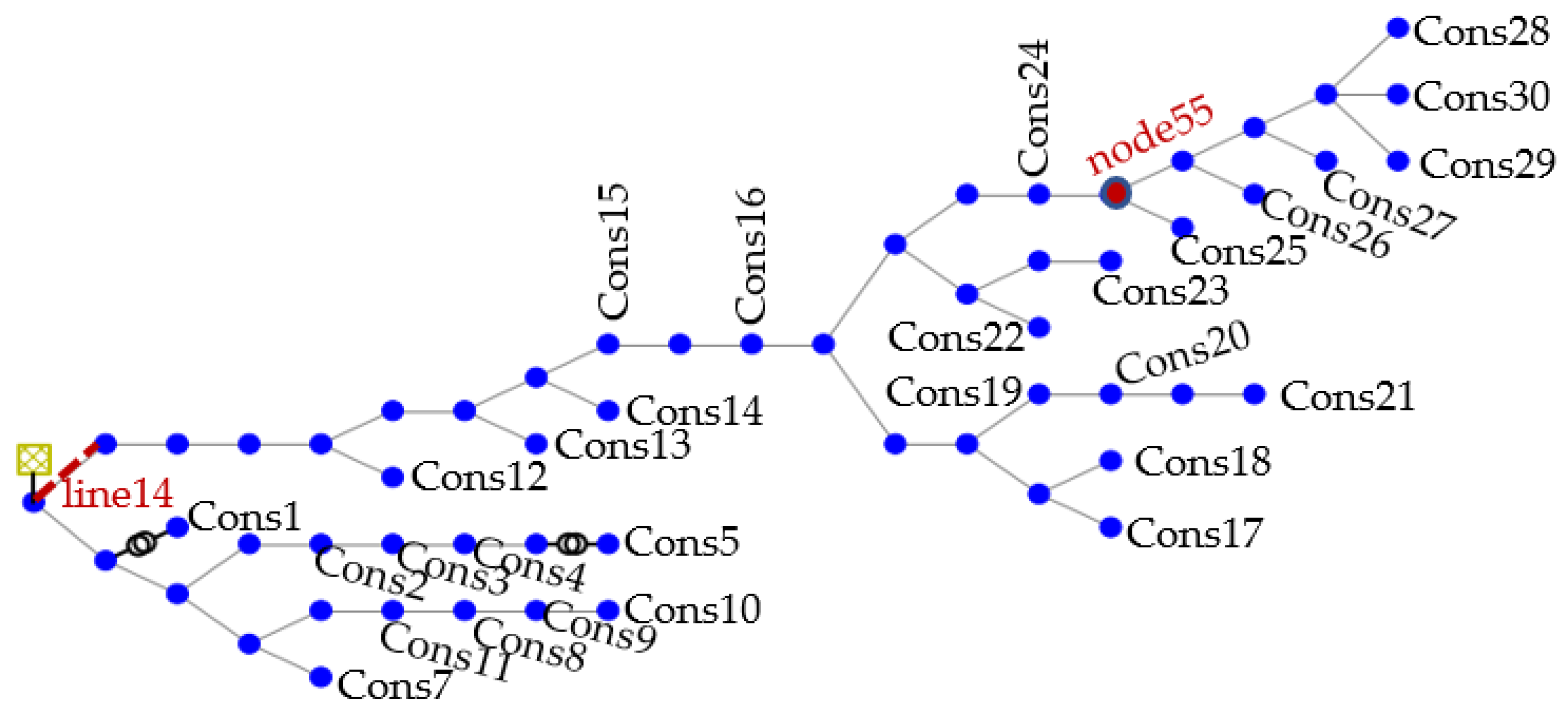
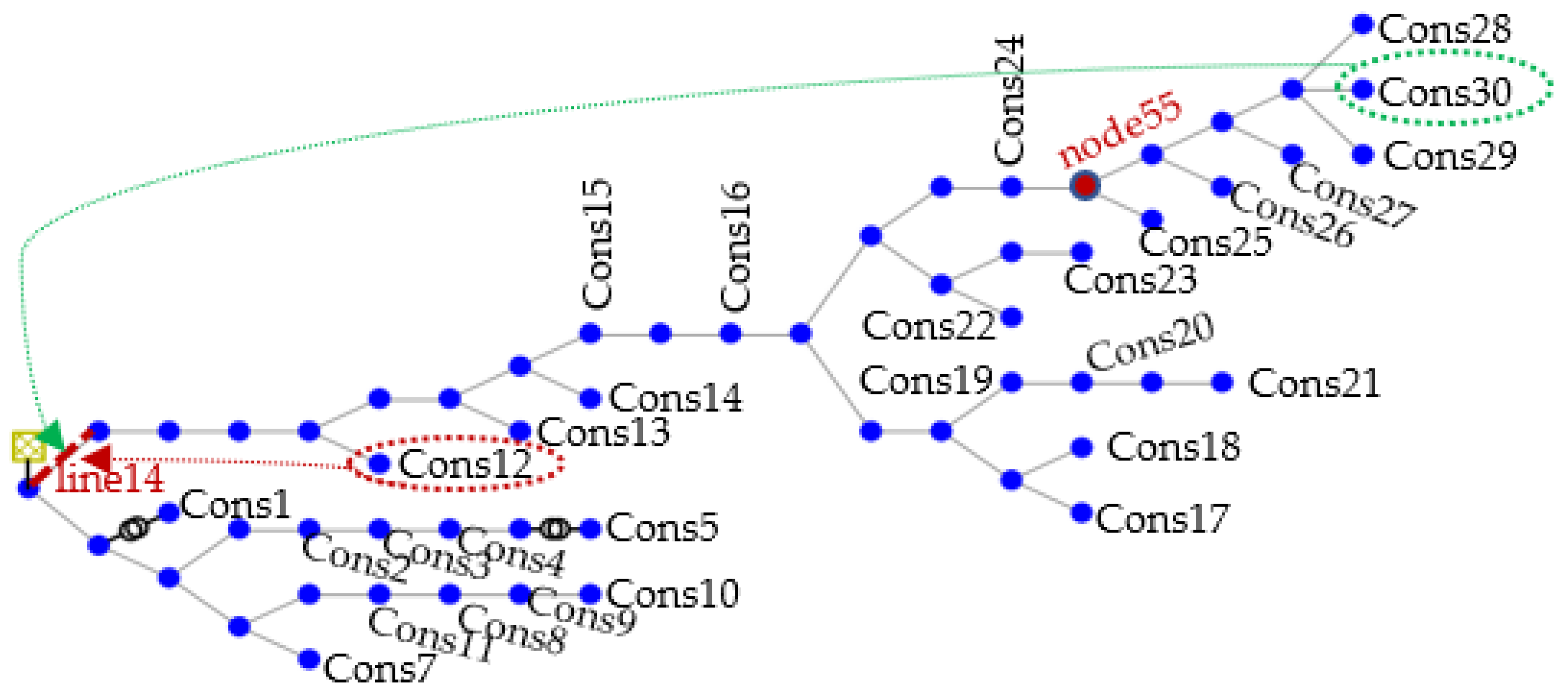
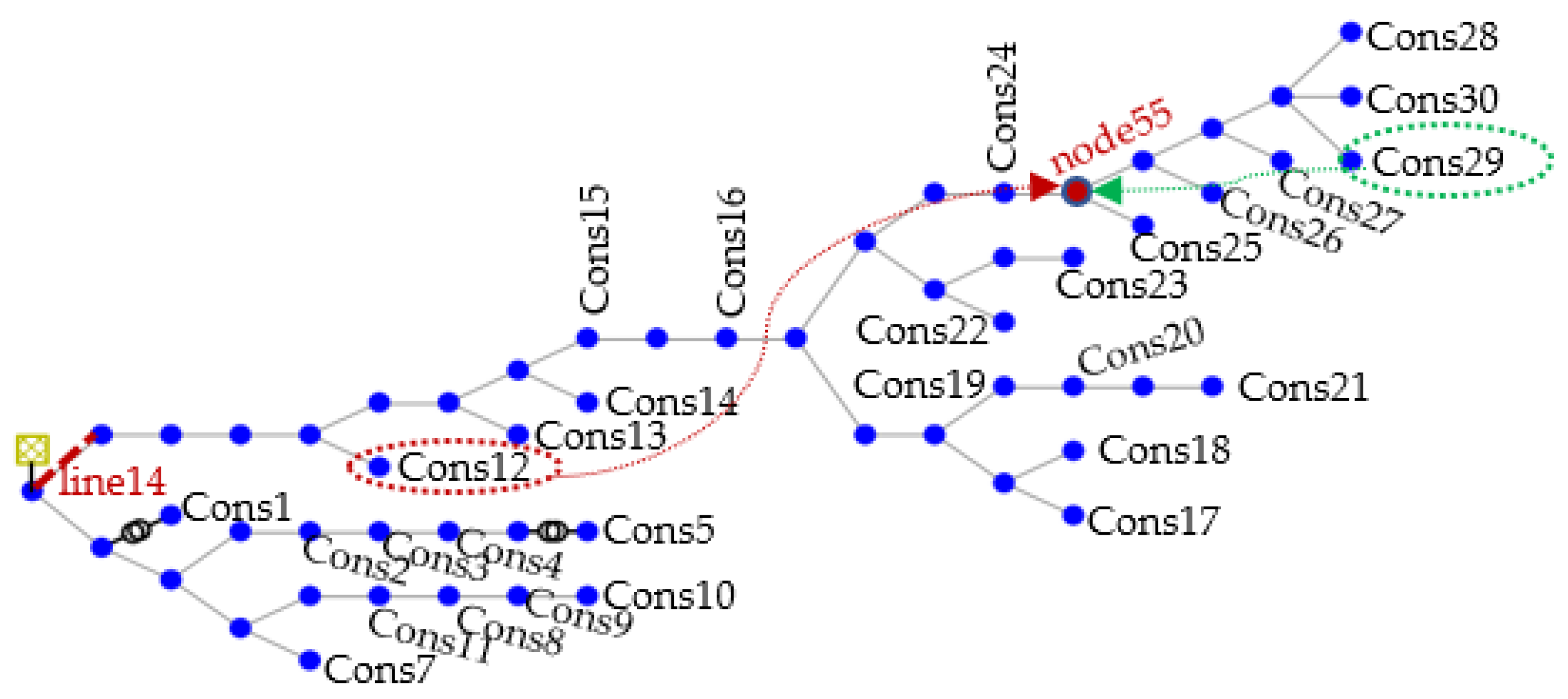
For the study, we chose a realistic topology of the MV grid feeder from Bosnia and Herzegovina, which is shown in Figure 1. It contains 54 lines with a total length of 20.11 km and 29 consumer nodes. The consumer nodes represent either individual consumers or aggregated consumers belonging to a 10/0.4 kV substation. In total, the distribution grid feeders include 1212 households, 125 other consumers including public lighting connected to the LV grid and 12 consumers connected to the MV grid. We assume that the flexibility providers act on the consumer nodes that are able to reduce the active energy consumption of the flexibility assets.

We use both historical data from 15-min smart meter readings of active and reactive power and data at the same resolution obtained from base load curves of individual consumption categories/groups for which there are no smart meters. Where there are no smart meters, we assume a constant power factor of 0.95. We increase the load on a higher distribution feeder by 3.5 times to simulate line congestion events on line 14, as shown in Figure 1. The total peak load is 8.28 MW.

3.2. Approach to Simulation

The power flow analysis is performed for the MV use case distribution grid shown in Figure 1. The distribution grid of the use case is modeled based on real grid topology data. First, power flow simulations are performed with initial load data at 15 min resolution. Based on the results, overload events for line overload and voltage control are isolated separately.

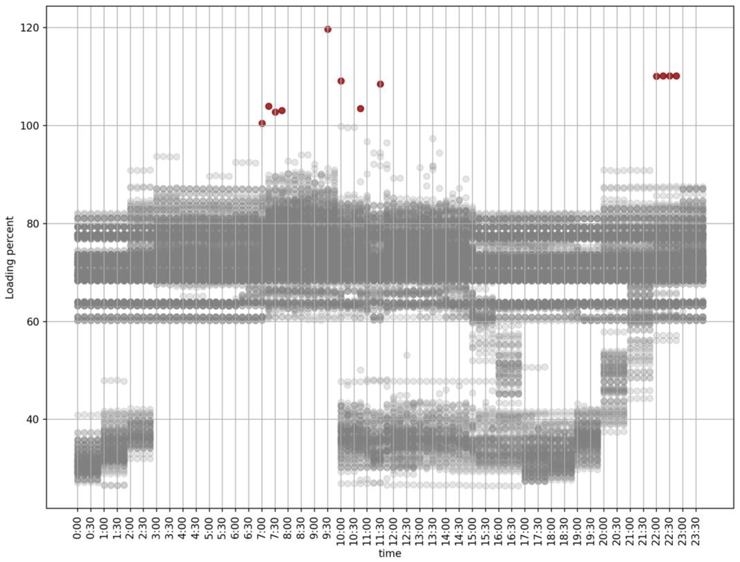
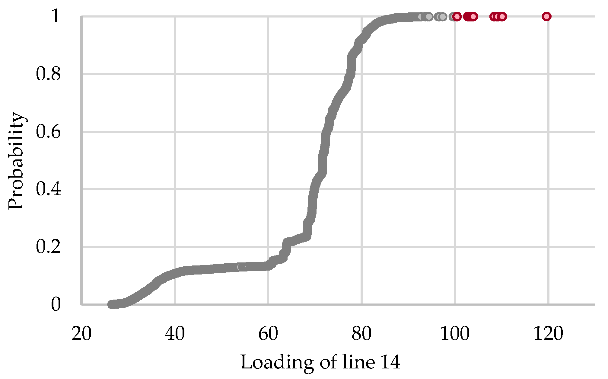
We found that line overload events are detected on line 14. The results of the power flow simulations in terms of the percentage load on line 14 for each interval of 15 min and the corresponding cumulative density function are shown in Figure 2 and Figure 3, respectively.

In Figure 2 and Figure 3, the grey dots represent the normal load on line 14 and the red dots represent the overloads on line 14. The load on line 14 is between 60% and 80% during approximately 80% of the observed period. The overload events occur 12 times during this period.

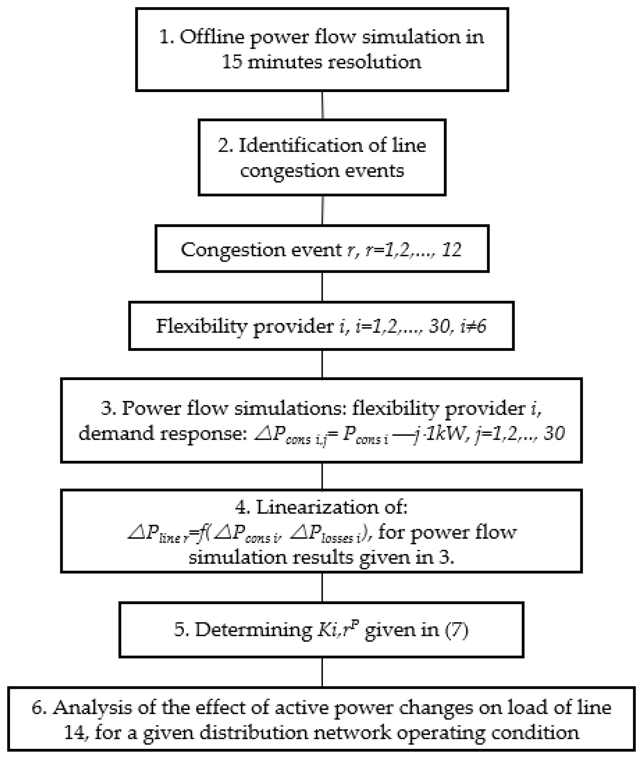
We assume that each flexibility provider is willing to provide a predetermined amount of DR power, with constraints specifying an amount approximately equal to the power demand of the load at a given time. For each detected line congestion event, we run power flow simulations for scenarios in which each of the 29 flexibility providers iteratively reduces its active power consumption by $\mathsf{\Delta }P=1 \mathrm{kW}$. If the baseline consumption of flexibility asset i is less than $\mathsf{\Delta }P·j$, the number of iterations is limited to j − 1. Otherwise, the number of iteration is 30. Here, j is the number of the iteration sequence.

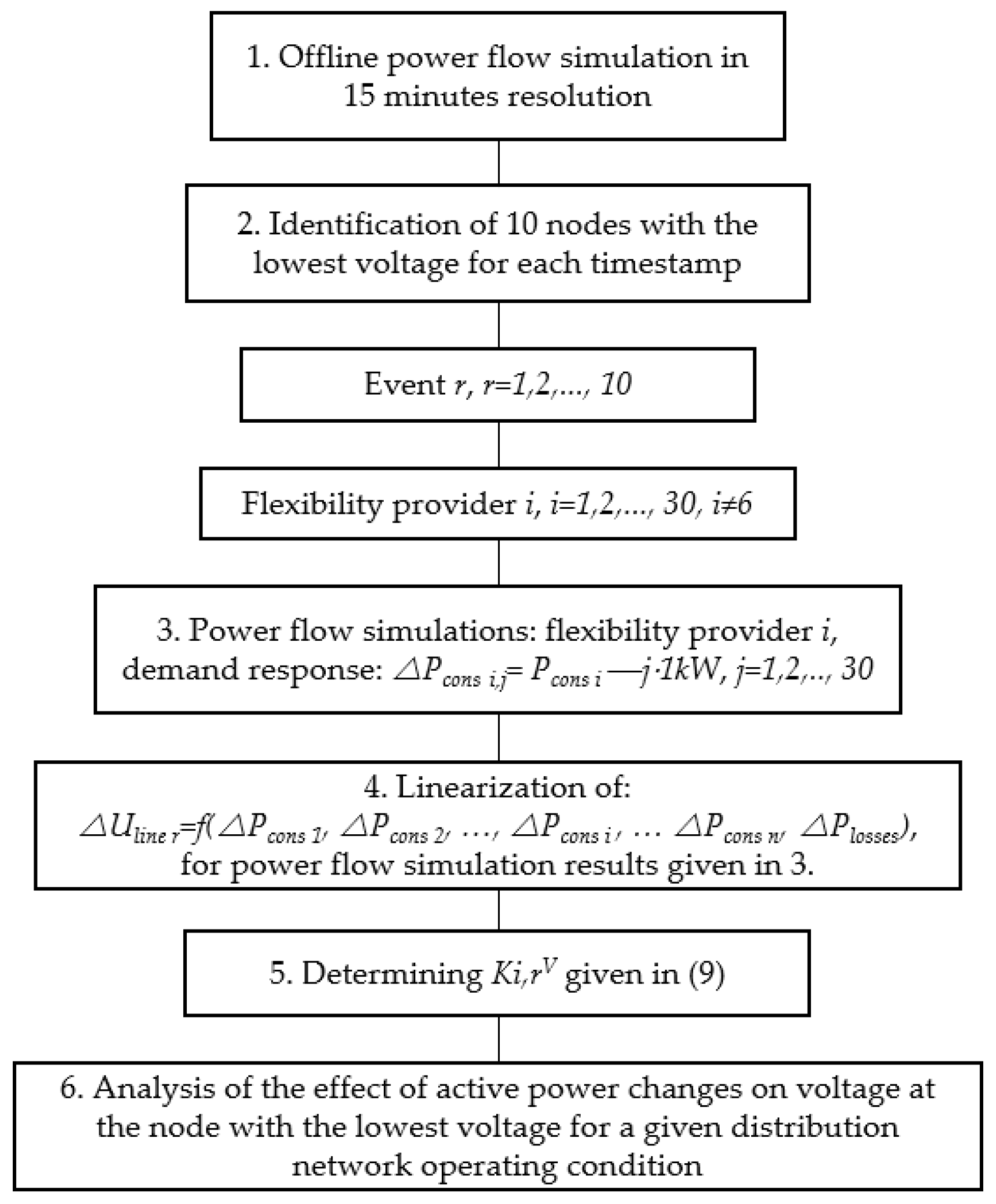
We study the impact of each flexibility provider/asset on the utilization of the congested line 14, both from the point of view of the influence of the location of the flexibility asset and from the point of view of the grid condition. In performing the analysis, we follow the algorithm shown in Figure 4.

After running the power flow simulations for each interval of 15 min for the initial data, we select 10 events where the lowest voltages occur. We store the location of node with lowest voltage in the grid for each event and present further analysis results for these locations.

We examine the impact of each flexibility provider/asset on increasing the voltage at the location with the lowest voltage by decreasing demand. The analysis is performed from the point of view of the influence of the location of the flexibility assets and the influence of the grid condition. The algorithm for performing the analysis is shown in Figure 5.

4. Results

4.1. Distribution Line Congestion Management

The results of the power flow analysis performed for the cases where each flexibility provider/asset provides service individually by reducing its load in defined number of iterations with step of ΔP = 1 kW, for a given grid state, is shown in Figure 6. The x-axis represents the demand-side power reduction and the y-axis represents the power change on the congested line 14.

The individual points in Figure 6 represent the results of the power flow simulations, with each color representing the results of the power flow simulation with respect to a flexibility provider/asset. The lines connecting the result points with respect to a flexibility provider/asset represent the result of the linearization process.

It should be noted that the linearized lines obtained for different flexibility providers/assets do not have the same line coefficients, indicating that the location of the flexibility asset has an impact on the relief of the congested line. It is also clear from the results shown in Figure 6, that the dependence between the change in load on the congested line and the change in the consumption of flexibility provider/asset is not linear but can be linearized with negligible error because the linearized line is very close to a single point that is a result of the power flow simulation.

The results of the linearization of the power flow simulation results described in Section 3, given as an ordered pair of coefficients of a best-fit line $\left[k_P, n_P\right]$, as well as the MSE calculated for the power flow simulation results and the values obtained using the relationship given in Equation (7) for each flexibility asset and an overload event shown in Figure 6, are given in

Table 1. Impact of change in active power consumption of flexibility provider/asset on change in load of a congested line for given line congestion event.

Flexibility Asset	Cons12	Cons14	Cons15	Cons16
$K_{i,14}^P$	[1.1607; 2.6816 × 10−6]	[1.2007; 3.0841 × 10−6]	[1.2069; 3.0790 × 10−6]	[1.2824; 5.2379 × 10−6]
MSE (%)	0.2419 × 10−4	0.2782 × 10−4	0.2778 × 10−4	0.4725 × 10−4
Flexibility Asset	Cons17	Cons18	Cons19	Cons20
$K_{i,14}^P$	[1.3180; 10.3143 × 10−6]	[1.3153; 7.0972 × 10−6]	[1.3223; 7.5435 × 10−6]	[1.3288; 8.2819 × 10−6]
MSE (%)	0.9300 × 10−4	0.6401 × 10−4	0.6803 × 10−4	0.7468 × 10−4
Flexibility Asset	Cons21	Cons22	Cons23	Cons24
$K_{i,14}^P$	[1.3335; 8.9465 × 10−6]	[1.3374; 7.8550 × 10−6]	[1.3384; 8.3596 × 10−6]	[1.3615; 9.4280 × 10−6]
MSE (%)	0.8067 × 10−4	0.7084 × 10−4	0.7538 × 10−4	0.8501 × 10−4
Flexibility Asset	Cons25	Cons26	Cons27	Cons30
$K_{i,14}^P$	[1.3679; 11.2043 × 10−6]	[1.3718; 12.1351 × 10−6]	[1.3786; 11.2901 × 10−6]	[1.4243; 18.0043 × 10−6]
MSE (%)	1.0101 × 10−4	1.0940 × 10−4	1.0178 × 10−4	1.6223 × 10−4

.

In our use case MV distribution grid, total power losses on the higher distribution feeder are approximately 7.5% in the initial grid condition. Based on the results shown in Table 1, the $n_{P,i}$ component of $K_{i,r}^P$ is much smaller than the $k_{P,i}$ component for the given grid condition r, so it can be neglected.

The results listed in Table 1 are illustrated in Figure 7. The flexibility provider/asset with the highest impact (Cons30) and flexibility asset with the lowest technical impact (Cons12) on congestion management on line 14 are marked with green and red colors, respectively. The difference between the impacts of these two flexibility providers/assets on congestion management on line 14 is 20%.

The results of the power flow analysis performed for the cases where a single flexibility provider/asset, Cons30, provides flexibility service by reducing its load in a certain number of iterations in steps of ΔP = 1 kW for different grid conditions, all indicated by an overload on line 14, including the process of linearization, are given in

Table 2. Impact of change in active power consumption of a flexibility provider/asset on change in load of a congested line for different line congestion events.

Event	3/4/2021 11:30	4/21/2021 10:45	4/26/2021 9:30	4/26/2021 10:00
$K_{i,14}^P$	[1.3945; 17.0715 × 10−6]	[1.4280; 18.4353 × 10−6]	[1.4243; 18.0043 × 10−6]	[1.4043; 17.4153 × 10−6]
MSE (%)	1.5383 × 10−4	1.6611 × 10−4	1.6223 × 10−4	1.5693 × 10−4
Event	5/25/2021 22:00	5/25/2021 22:15	5/25/2021 22:30	5/25/2021 22:45
$K_{i,14}^P$	[1.4548; 19.3907 × 10−6]	[1.4553; 19.4073 × 10−6]	[1.4553; 19.4082 × 10−6]	[1.4553; 19.4077 × 10−6]
MSE (%)	1.7471 × 10−4	1.7486 × 10−4	1.7486 × 10−4	1.7486 × 10−4
Event	5/26/2021 7:00	5/26/2021 7:15	5/26/2021 7:30	5/26/2021 7:45
$K_{i,14}^P$	[1.4051; 17.5751 × 10−6]	[1.4206; 18.0946 × 10−6]	[1.4153; 17.9201 × 10−6]	[1.4166; 17.9650 × 10−6]
MSE (%)	1.5836 × 10−4	1.6304 × 10−4	1.6147 × 10−4	1.6187 × 10−4

and shown in Figure 8.

In Figure 8, the x-axis represents the demand-side power reduction and the y-axis represents the power change on the congested line 14. The individual points in Figure 8 represent the power flow simulation results, with each color representing the power flow simulation results with respect to a grid condition. The lines connecting the points with respect to the grid condition represent the result of the linearization process.

Note that the linearized lines obtained for different grid states do not have the same line coefficients. The linearized lines are very close to a single point obtained from the power flow simulation results for one grid state. From the results in Table 2, we can conclude that the influence of a flexibility provider/assets varies by up to 5% depending on the grid condition.

4.2. Voltage Control

The results of the power flow analysis performed for the cases where each flexibility provider/asset performs individually by reducing its load for a given number of iterations in increments of ΔP = 1 kW for a given grid state are shown in Figure 9. The x-axis represents the demand-side power reduction and the y-axis represents the voltage change at the node with the minimum voltage.

The individual points in Figure 9 represent the results of the power flow simulation, with each color representing the results of the power flow simulation with respect to a flexibility provider/asset. The lines connecting the result points with respect to a flexibility provider/asset represent the result of the linearization process.

It should be noted that the linearized lines obtained for the different flexibility assets have significantly different coefficients. It is also clear that the dependence between the voltage change at the node with the minimum voltage and the consumption at a node of the network feeder is not linear but can be linearized with a negligible error since the linearized line is very close to a single point that is a result of the power flow simulation.

The results of linearizing of the power flow simulation results described in Section 3, given as an ordered pair of line coefficients $\left[k_{V,i}, n_{V,i}\right]$, as well as the MSE calculated for the power flow simulation results and the values obtained using the relationship given in Equation (9) for each flexibility asset and the voltage violation event shown in Figure 9, are shown in

Table 3. Impact of change in active power consumption of flexibility provider/asset on change in voltage at a node with the smallest voltage for given grid condition.

Flexibility Asset	Cons12	Cons14	Cons16	Cons17
$K_{i,55}^V$	[0.0132; 0.0434 × 10−6]	[0.0165; 0.0590 × 10−6]	[0.0255; 0.1373 × 10−6]	[0.0283; 0.2777 × 10−6]
MSE (%)	0.0039 × 10−4	0.0053 × 10−4	0.0124 × 10−4	0.0250 × 10−4
Flexibility Asset	Cons18	Cons19	Cons20	Cons21
$K_{i,55}^V$	[0.0282; 0.1974 × 10−6]	[0.0284; 0.2088 × 10−6]	[0.0286; 0.2287 × 10−6]	[0.0288; 0.2466 × 10−6]
MSE (%)	0.0178 × 10−4	0.0188 × 10−4	0.0206 × 10−4	0.0222 × 10−4
Flexibility Asset	Cons23	Cons24	Cons25	Cons26
$K_{i,55}^V$	[0.0323; 0.2514 × 10−6]	[0.0408; 0.3566 × 10−6]	[0.0414; 0.4248 × 10−6]	[0.0425; 0.4692 × 10−6]
MSE (%)	0.0227 × 10−4	0.0322 × 10−4	0.0383 × 10−4	0.0423 × 10−4
Flexibility Asset	Cons27	Cons29	Cons30
$K_{i,55}^V$	[0.0477; 0.4881 × 10−6]	[0.0885; 1.5721 × 10−6]	[0.0721; 1.1129 × 10−6]
MSE (%)	0.0440 × 10−4	0.1416 × 10−4	0.1003 × 10−4

.

Based on the results presented in Table 3, a component $n_{V,i}$ of $K_{i,r}^V$ for the given grid condition r is significantly smaller than the component $k_{V,i}$, so it can be neglected.

Figure 10 illustrates the results listed in Table 3, with the flexibility provider/asset with the greatest impact on voltage increase, labelled Cons29, at the node with the lowest voltage, labelled node55, highlighted in green, and the flexibility provider/asset with the least impact, labelled Cons12, highlighted in red.

The results of the power flow analysis performed for the cases where a single flexibility provider/asset provides its service by reducing its load in a certain number of steps of ΔP = 1 kW for different grid conditions, i.e., voltage violation events, all indicated by undervoltage at the node with the minimum voltage, are shown in Figure 11. The x-axis represents the demand-side power reduction and the y-axis represents the voltage change at the node with the minimum voltage.

The individual points in Figure 11 represent the results of the power flow simulation, with each color representing the results of the power flow simulation with respect to a grid condition. The lines connecting the result points with respect to the grid condition represent the result of the linearization process. The linearized lines obtained for different grid conditions do not have the same line coefficients. The linearized lines are very close to a single point obtained from the power flow simulation results for one grid state.

The results of the linearization of the power flow simulation results described in Section 3, given as an ordered pair of line coefficients $\left[k_V, n_V\right]$, as well as the MSE calculated for the power flow simulation results and the values obtained using the relationship given in Equation (9) for each voltage violation event shown in Figure 11, are given in

Table 4. Impact of change in active power consumption of a flexibility provider/asset (Cons30) on change in voltage at node with the lowest voltage.

Event	5/25/2021 22:30	5/25/2021 22:45	5/25/2021 22:15	5/25/2021 22:00	4/26/2021 9:30
$K_{i,r}^V$	[0.0721; 1.1129 × 10−6]	[0.0721; 1.1129 × 10−6]	[0.0721; 1.1129 × 10−6]	[0.0721; 1.1120 × 10−6]	[0.0698; 1.0156 × 10−6]
MSE (%)	0.1003 × 10−4	0.1003 × 10−4	0.1003 × 10−4	0.1002 × 10−4	0.0915 × 10−4
Event	4/21/2021 10:45	5/26/2021 7:15	5/26/2021 7:45	5/26/2021 7:30	4/26/2021 10:00
$K_{i,r}^V$	[0.0709; 1.0617 × 10−6]	[0.0704; 1.0404 × 10−6]	[0.0702; 1.0340 × 10−6]	[0.0702; 1.0317 × 10−6]	[0.0692; 0.9927 × 10−6]
MSE (%)	0.0957 × 10−4	0.0937 × 10−4	0.0932 × 10−4	0.0930 × 10−4	0.0894 × 10−4

. From the results in Table 2, it can be seen that the difference between the influences of a flexibility provider/asset is approximately 3%, depending on the grid condition.

5. Discussion

In this paper, we evaluate the methodology proposed in Section 3 by modeling a Python-based simulator and testing it on a use case from Bosnia and Herzegovina based on the real topological data of the medium-voltage distribution grid and on the real electricity demand data and a universal demand curve where smart meter data is missing. With this approach, we analyze a realistic scenario as opposed to studies based on synthetic use cases [43].

In our use case, flexibility services are provided in the form of DR. Based on the premise that flexibility assets can provide services by changing active or reactive power [35], in this analysis we restrict ourselves to active power, following the approach described in [41].

As stated in Section 3, following the idea of introducing PTDFs [37,38] and VSCs [38,41,42], the coefficients of the impact of flexibility assets on line congestion management and voltage control are calculated based on the results of power flow simulations performed for a MV distribution grid.

In addition to the impact of demand-side active power changes on voltage at a given node using possible flexibility options in a defined range of flexibility services described in [41], the approach presented in this paper considers both the impact of demand-side active power changes on line congestion management and voltage control. The power flow analysis is performed for the cases where each flexibility provider/asset offers an individual reduction in active power demand, for a given grid condition.

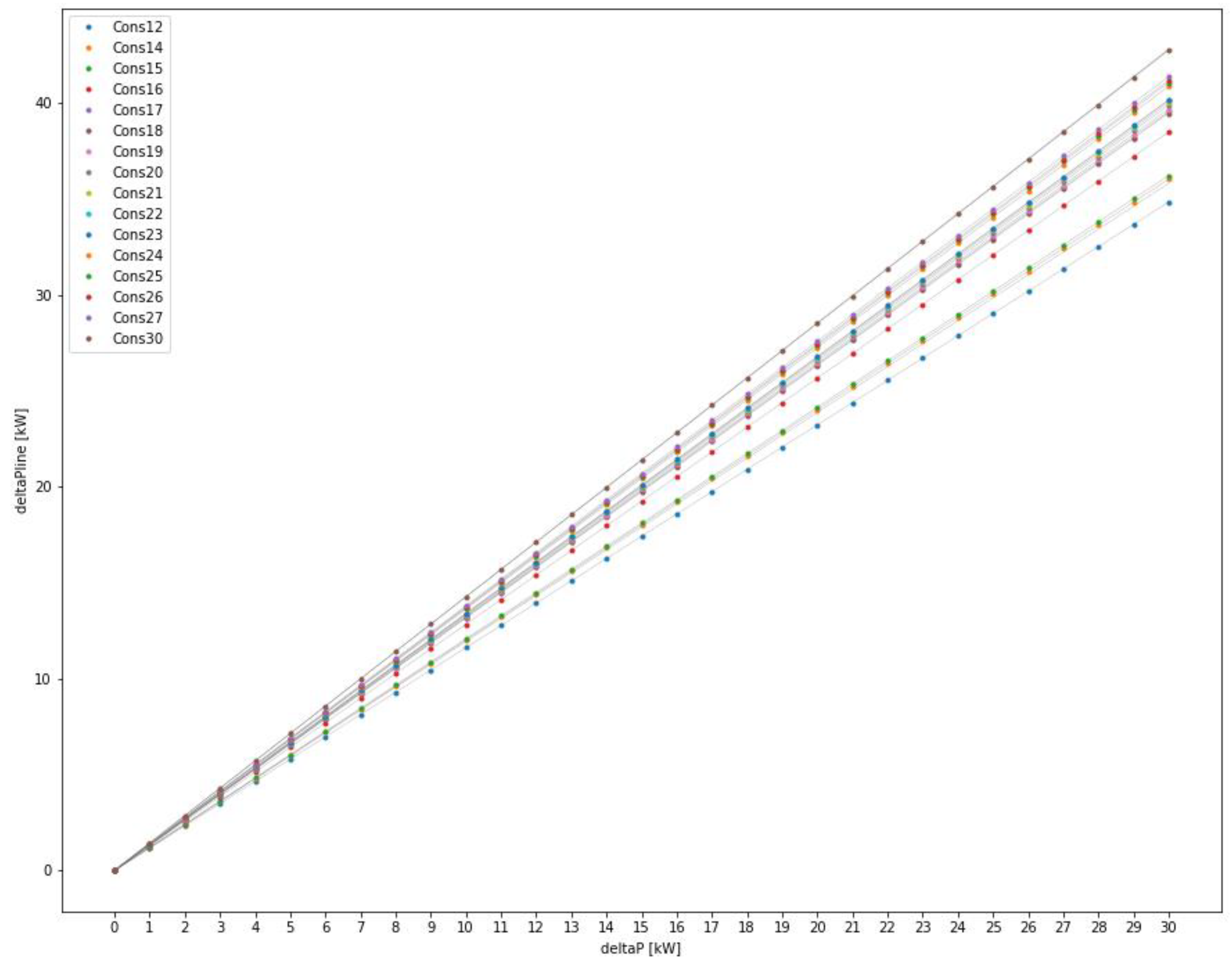
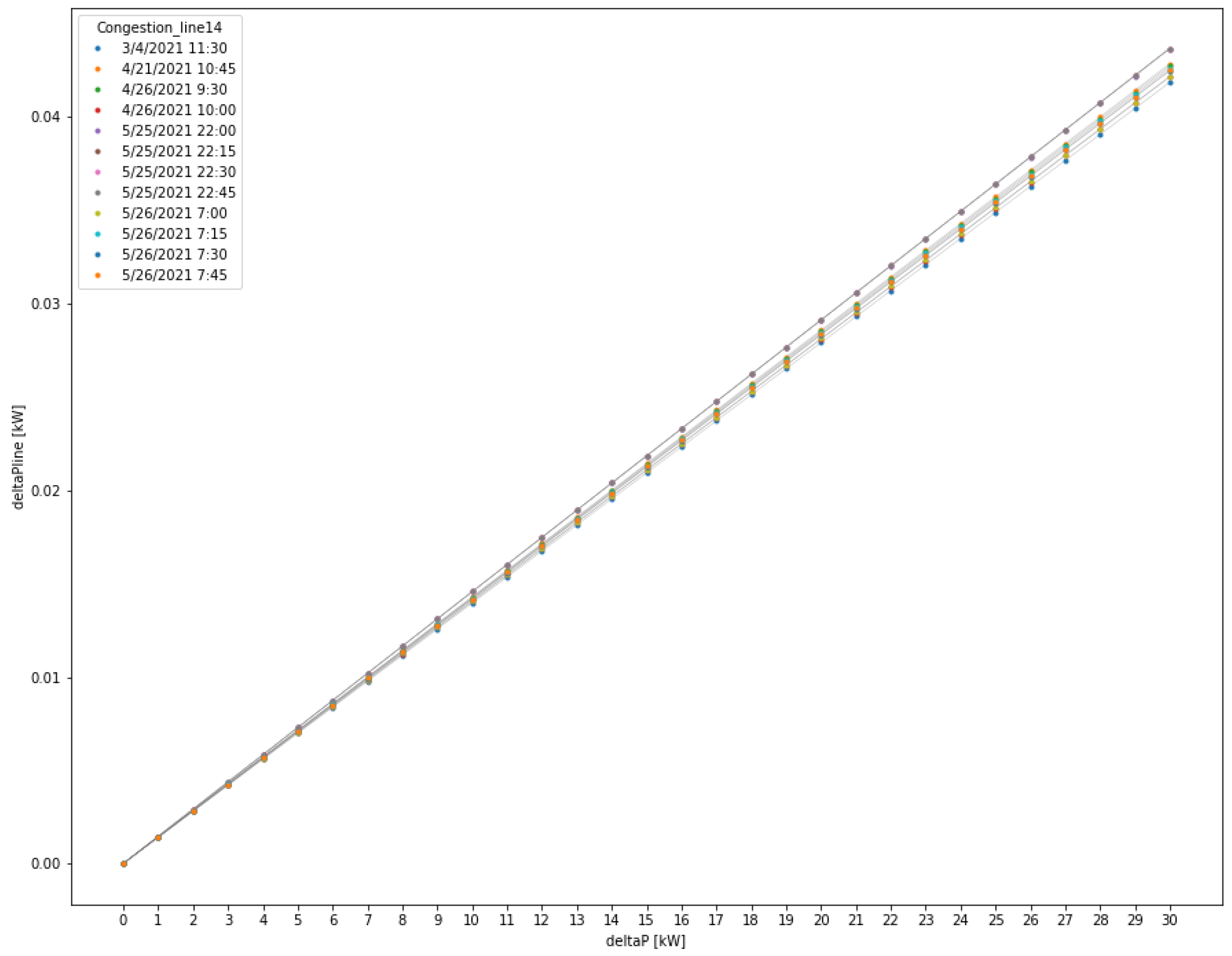
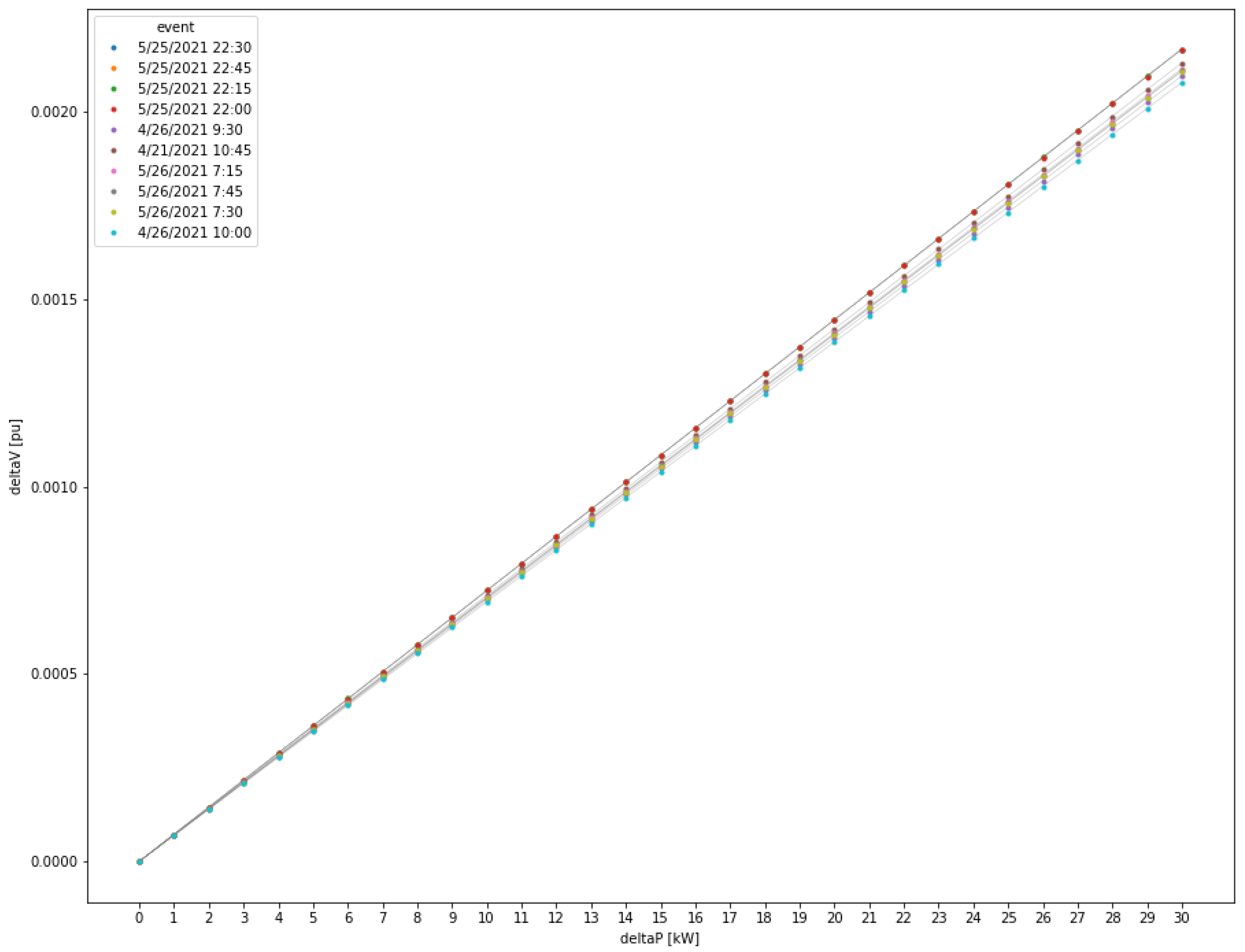
Figure 6 shows the results of the sensitivity analysis of the impact of the change in active power demand of each flexibility provider/asset on the change in the load of the congested line for the case where each flexibility provider/asset provides a flexibility service by reducing its active power demand for a given grid condition. Figure 8 shows the results of the sensitivity analysis of the impact of the change in the active power demand of the flexibility provider/asset on the change in the load of the congested line for the case where a single flexibility provider/asset provides a flexibility service by reducing its active power demand for different grid states. In Figure 6 and Figure 8, the x-axis represents the demand-side power reduction and the y-axis represents the active power change on the congested line 14.

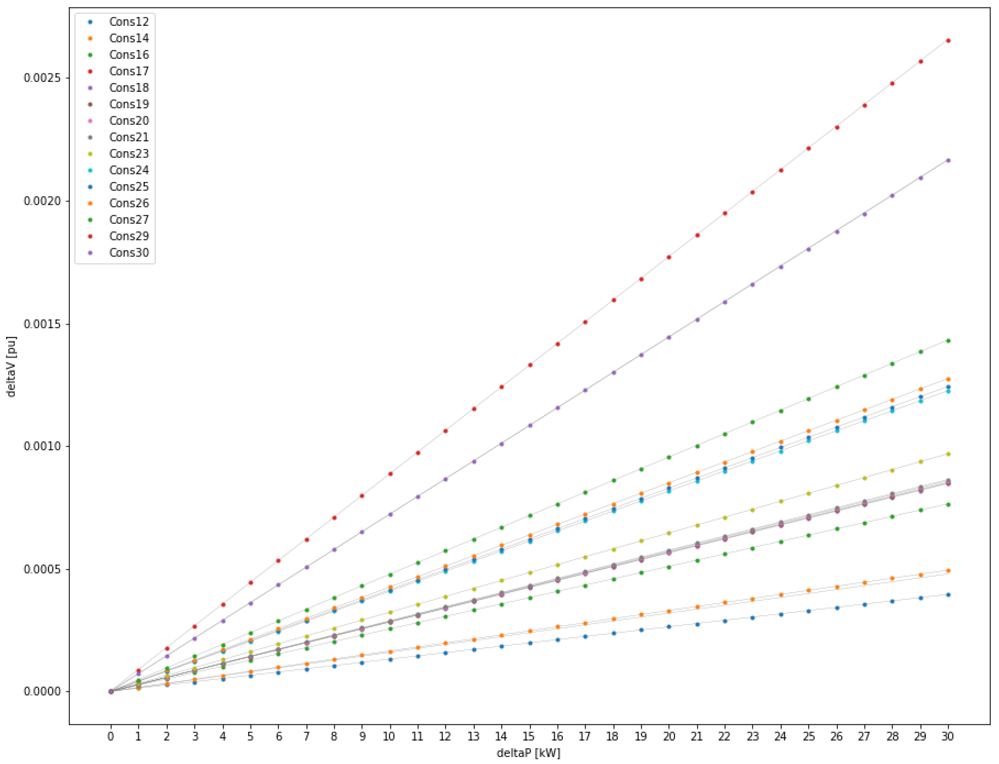
Figure 9 shows the results of the sensitivity analysis of the impact of the change in active power demand of each flexibility provider/asset on the change in voltage at the node with the minimum voltage in the distribution feeder for the case where each flexibility provider/asset provides a flexibility service by reducing its active power demand for a given grid condition. Figure 11 shows results of the sensitivity analysis of the impact of the change in the active power demand of the flexibility provider/asset on the change in the voltage at the node with the minimum voltage in the distribution feeder for the cases where a single flexibility provider/asset provides a flexibility service by reducing its active power demand for different grid states. In Figure 9 and Figure 11, the x-axis represents the demand-side power reduction and the y-axis represents the voltage change at the node with the minimum voltage.

Following the approach in [41], the results obtained in this paper show a linear dependence between the voltage change at a given node and the demand change at the consumer node but also indicate that the grid condition affects such a line. We also show a linear dependence between the change in line load and the change in active power consumption of the flexibility asset. From the results presented in Table 1, Table 2, Table 3 and Table 4 in Section 4, the MSE of each line is at least${10}^{-4}$, which confirms the justification for introducing linearization.

The results in Table 1 and Table 3, shown in Figure 6 and Figure 9, respectively, confirm that not all flexibility assets have the same technical impact on congestion management and voltage control. We conclude that location of the flexibility asset has an impact on the resolution of line congestion and voltage violations, while the impact is even larger for voltage control.

In addition, the results in Table 2 and Table 4, shown in Figure 8 and Figure 11, respectively, indicate that the effect of a demand-side active power change on either the voltage at a node or a line load in the distribution grid depends on the condition of the distribution grid, i.e., on the current parameters of distribution network. However, comparing the results of the technical impact of flexibility assets on line congestion management and voltage control for different distribution system conditions, we conclude that the relative difference in the impact of flexibility assets changes little regardless of the condition of the distribution system.

The impact of changing the demand of Cons1, Cons2, Cons3, Cons4, Cons5, Cons7, Cons8, Cons9, Cons10, and Cons11, which belong to the lower distribution feeder, on the load of line 14, which belongs to the upper distribution feeder, is almost zero because both distribution feeder lines are connected to the same slack bus.

We consider the utility of locational information in the local flexibility market in addition to the technical information about flexibility resources, contained in the flexibility register, such as location, approved capacity limits, duration, ramp rates, activation mode, flexibility assets, and baseline information [35]. The line coefficients $n_P$ and $n_V$ are negligible compared to $k_P$ and $k_V$, respectively, confirming the correctness of using PTDFs and VSCs for quantifying the location of flexibility resources for flexibility service in the distribution grid.

In addition to the location information derived from the point of connection, we propose additional information for the flexibility register on the impact of the flexibility asset on line congestion management and voltage control. We believe that such information can be useful for weighting bids in the local flexibility market according to respective technical impacts [34].

6. Conclusions

This paper addresses the dependence between the location of the DR provider and the efficiency of grid congestion management, including the impact of the operation condition of the distribution grid on the DR effect. We introduce flexibility impact information to exploit flexibility to support market-based congestion management in the distribution system.

The paper proposes to use the assumption of linear dependence between the demand-side active power and line load, i.e., voltage at nodes, in the distribution system. It is proposed to use the coefficients of these linearized lines, given in the form of PTDFs and VSCs, as additional information in the flexibility register, both for voltage regulation and for line congestion management. The results obtained in this paper confirm that the methodology for determining the impact of active power changes on the demand side on congestion management in the distribution system should take into account the impact of power loss changes, as it was also stated in [38].

In the local flexibility market, flexibility products are procured to solve a specific congestion problem of the DSO. An economically optimal solution to solve the congestion problem in the distribution system should consider the amount of flexibility products that can solve the congestion problem. The analysis of possible solutions to solve the congestion problem should consider the quantification of the location of the flexibility sources on the flexibility service, i.e., the technical impact of each flexibility provider on solving the congestion problem. Using the merit order approach based only on bid prices may lead to an incorrect solution in terms of economic optimality.

Providing the flexibility register with information on the weighting of each flexibility asset in terms of its respective technical effect is useful for the phase of evaluating the weighting of flexibility bids without repeating power flow simulations, and makes the information transparent to all actors in the flexibility market.

Our further research will focus on information modeling related to efficient use of available energy sources and increasing the diversity of energy services to support the process of local electricity market development.