Assessing the Energy Efficiency Gains and Savings in China’s 2060 Carbon-Neutral Plan

Abstract

At the end of 2020, the Chinese government announced the pledge to become carbon neutral in the year 2060. Simultaneously, quality growth objectives were established, which were environmentally friendly and promoted the health and wellbeing of the population. The first objective of this study is to assess the gains in energy efficiency and the savings in energy demand that this commitment implies. Secondly, the feasibility of achieving these objectives of savings and efficiency increases is discussed based on an international analysis. The method is based on a quantitative estimate of the primary energy demand throughout the period from 1965 up to the year 2060. For this purpose, long historical series taken from reliable international sources are analyzed. The methodology applied to estimate and project future energy demand is new and based on several steps: The first consists of analyzing the trends of the series and estimating the relationships between them using a robust procedure. Secondly, equilibrium relationships are estimated, which avoids the eventual instabilities involved in the estimation of dynamic models. The third characteristic is based on the bootstrap, estimating and simulating the model by selecting random samples of different sizes from the available dataset. The simulations generate a complete probability distribution for the expected energy demand, which also allows for carrying out a risk analysis, assessing the risk of the demand becoming significantly larger than the expected average. The first result obtained is that the primary energy demand forecast for 2060 is much higher than the demand of the official forecasts by almost three times. However, taking into account the objective to replace 85% of fossil sources with renewables, this discrepancy is greatly reduced and becomes approximately 50% higher than the official forecast. If the savings analyzed in relevant international references are accounted for, then an additional reduction of even up to 40% of this demand could be achieved, so that the final demand would fall further, close to official forecasts. The main and final conclusion is that although the objective of making the Chinese economy carbon neutral by 2060 is feasible, it implies a radical transformation that will necessarily require a determined and unwavering political commitment throughout the entire period considered.

1. Introduction

At the end of 2020, the Chinese government announced a commitment to become carbon neutral by the year 2060. In addition, it was expected that the peak of carbon emissions would be reached before 2030. This would all be accompanied by a change in the policy of growth, oriented towards quality growth that is environmentally friendly and focused on the people’s wellbeing [1]. Although not many details were given at the time of the pledge announcement, it is interesting to note that a publication close to the Chinese government [2] indicated, among other things, that coal was not going to be abandoned, but that it would be coupled with a policy of Carbon Capture Utilization and Storage (CCUS). They also pointed out that measures would be adopted to develop the carbon emissions market and emission limits, and simultaneously underlined the commitment to reach a circular economy and the greening of the economy. The pledge was not accompanied at the time of its announcement by a detailed plan to implement it. However, it was internationally accepted and received with surprise, and with relief, since China emits approximately 30% of the world’s greenhouse gases (GHGs). Because of this, any plan to cap world GHG emissions so that the temperature does not increase, following the lead of the IPCC, involves the Chinese economy in an essential and primary way.

The international organizations specializing in energy analysis valued this commitment very positively, although they underlined the enormous difficulty of carrying it out. The IEA [3], for example, stressed the need to increase innovation, as well as electrification in transport and buildings. It also noted that the targets were within the financial possibilities of the Chinese economy. The IEA also stressed that it was necessary to adapt the pace of transformation to the interests of shareholders and consumers, to allow them to adapt to the changes. On its part, Irena [4], in addition to the usual advice on accelerated renewable energy (RE) deployment, made the following recommendations: (a) develop a detailed plan for the energy transformation of all sectors of the economy; (b) accelerate the phase-down of coal as an energy source; (c) prioritize cities as champions of low-carbon living and, simultaneously, prioritize a system based on distributed energy generation; (d) contribute to making the electricity system more flexible by making urban energy demand more responsive to renewable generation. Irena’s approach is especially interesting because it is in line with the development of distributed energy and the abandonment of the centralized system based on fossil fuels. This is an important difference in this report from that of the IEA.

After this announcement, various official Chinese bodies began to publish increasingly detailed reports on the roadmap for carrying out the plan. One of the best-known was developed by Tsinghua University [5], although the horizon considered in this case was the year 2050. Broadly speaking, this plan clarified that the objective was to reach approximately 85% RE in that year—including nuclear energy—and 15% from fossil energies, whose emissions would be dealt with by the CCUS implementation. The roadmap also assumed that the final energy demand would continue to increase slightly until 2030 and to decrease thereafter, reaching in 2050 almost the same value as in 2020. A further similar scenario was published by another Chinese institute [6], although the final energy demand estimates were somewhat less restrictive. Recently, Sinopec [7] also published some detailed scenarios, perhaps somewhat more realistic to the extent that they assume a slight increase in final energy demand in 2060—although not by much more.

The Chinese government’s announcement also drew, and continues to draw, a lot of attention in the academic world, although it has mainly been Chinese authors who have analyzed it concluding, in general, that it is feasible. For example [8], although their analysis is fundamentally descriptive, it stresses the need to stop the development of new coal mines and accelerate as much as possible the deployment of renewable energies. In [9], they used a 19-year database (2001; 2019) to estimate a disaggregated demand model for various types of energy and predict future demand up to 2060. The estimate was based on the method of least squares, including several parameters that were estimated a priori. On the other hand, in this study, to make the projection it was assumed that the efficiency in the demand for energy of each type would follow the official forecasts. Thus, finally, they obtained that the prediction was consistent with the assumptions of the government, so that the expected energy demand will turn out to be in 2060 approximately the same as that of 2020. In [10], they carried out a demand analysis, also up to 2060, based on a breakdown into 30 Chinese provinces. These authors took the official forecasts for energy intensity as the dependent variable in the prediction period. From there, they estimated a model, and the result they obtained was that the expected aggregate energy demand in 2060 will be approximately equal to that of 2020, confirming the official forecasts. Perhaps the most interesting aspect of this study is that they analyzed the demands of each province independently. In [11], they started from a standard emissions equation that was broken down into several explanatory factors. In turn, these factors and their future evolution were predicted using a type of machine-learning model—a genetic algorithm with a long short-term memory approach (GA-LSTM). These authors used a sample from 2000 to 2019, i.e., 20 observations, to estimate these models. Furthermore, they only estimated with 85% of the sample, so ultimately, they used only 17 observations to estimate an independent machine-learning model for each variable. The final conclusion was that the objectives for 2030 can be achieved, although for 2060 they are less optimistic. In [12], they developed an emissions model based on growth, but measured through a series of indicators that included quality, i.e., ‘quality growth’ as the authors put it. The model used was the Environmental Kuznets Curve (EKC). These authors concluded that neutrality in carbon emissions can be achieved before 2050 but that the demands on quality growth are very high. An issue with this model is that being a quadratic function, beyond the point where zero emissions are reached, it implies that they become increasingly negative, something not feasible in the long run. In [13], they applied a grey-type model to predict the demand for non-renewable energy. Although they only extrapolated it to 2026, they concluded that it would continue to grow, a result that perhaps calls into question the official forecasts. In [14], they emphasized that a country like the United States, currently the world’s second largest emitter of greenhouse gases, has taken nearly 90 years to reach the point of reducing emissions while maintaining economic growth. However, China is expected to reach that point much sooner, implying that the demands on China are much higher than they have been for other Western countries. This, following the authors, underscores the difficulty and effort of the neutrality commitment. In [15], they established a predictive model based on a disaggregated analysis for 30 Chinese provinces, and analyzed several possible scenarios of population, technology, and economy growth. To analyze their emission models for each province, they used the official forecasts, from which they estimated the model, so that their final outcome was that the official forecast can be met, since the decreases implied by the estimates are considered viable. From another more limited perspective, [16] analyzed the demand for the critical minerals necessary for the planned deployment of RE, especially photovoltaic (PV), wind, and electric vehicles (EVs). The most salient conclusion from this study was the limited cobalt supply, which may make it difficult to carry out plans for the deployment of EVs. This also matches the general estimates made for the world [17].

In summary, the general conclusion, both from international organizations and from academic studies, is that the objective of neutrality announced by the Chinese government is feasible, although it implies a series of important transformations of the Chinese energy system. It should also be noted that all these studies are based on very short historical series, generally a maximum of 20 years. In addition, the methods applied are either excessively simple and based on a direct application of ordinary least squares, to more or less disaggregated models, or they even apply machine-learning methods to rather short databases, with a limited suitability for this type of estimation approach. In addition, almost all the studies introduce in one way or another the official forecasts of efficiency gains within their forecasts, which, although not necessarily incorrect, does not provide an independent assessment of the feasibility of those forecasts.

In this context, therefore, the objectives of this study are the following:

(1)

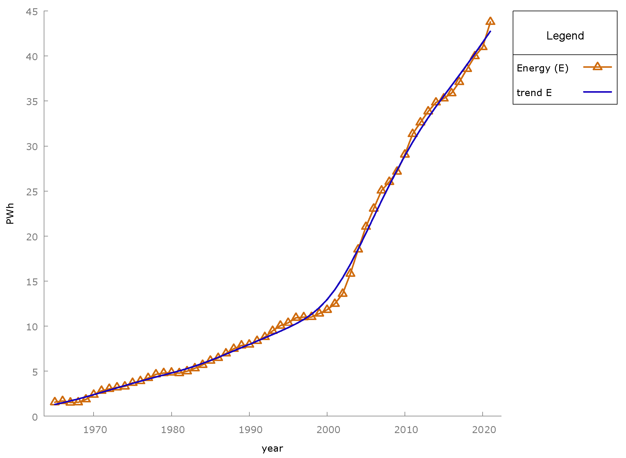
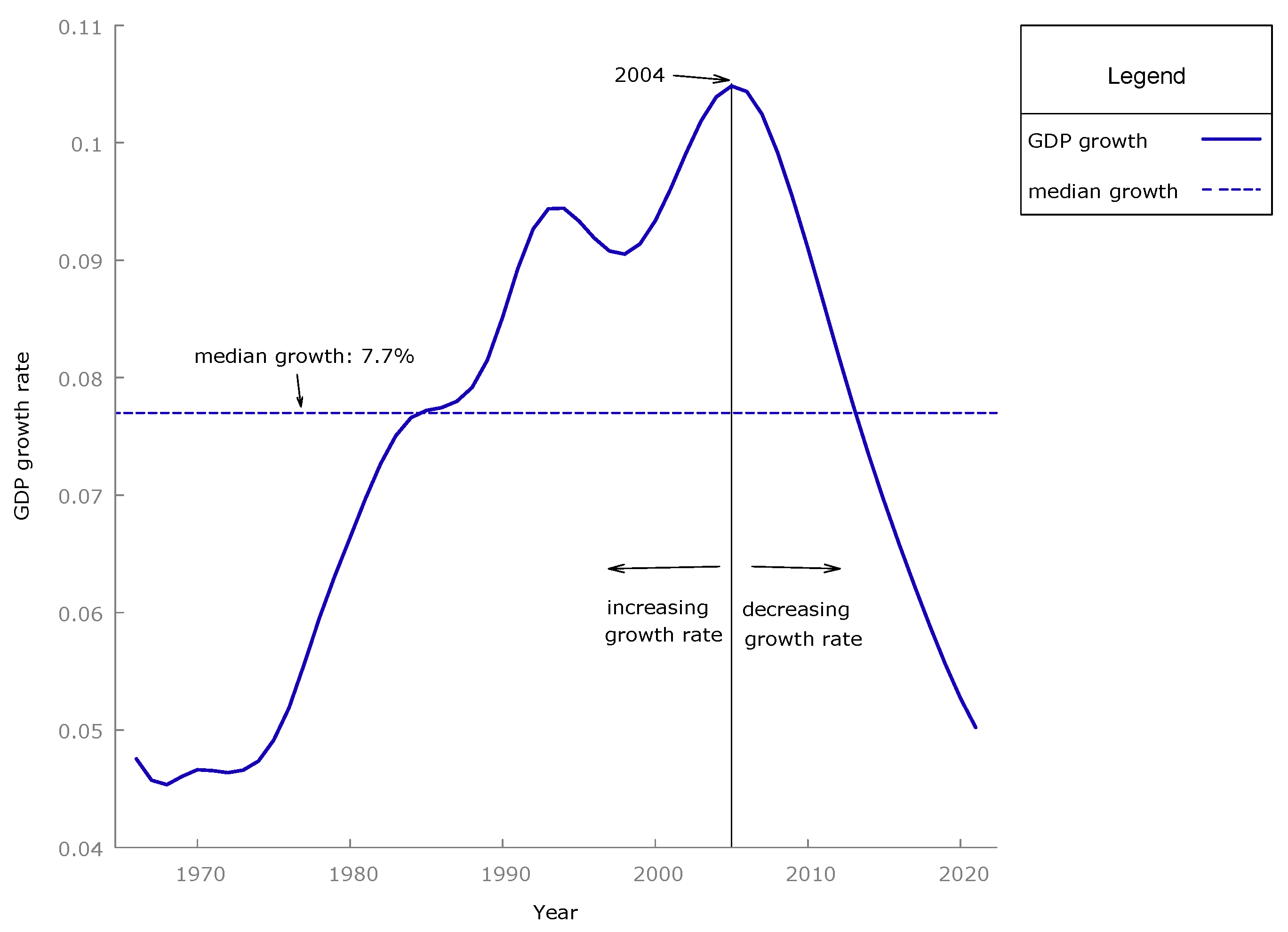
Quantitatively estimate an aggregate model for the primary energy demand in China, based on long historical series and using a novel estimation methodology.

(2)

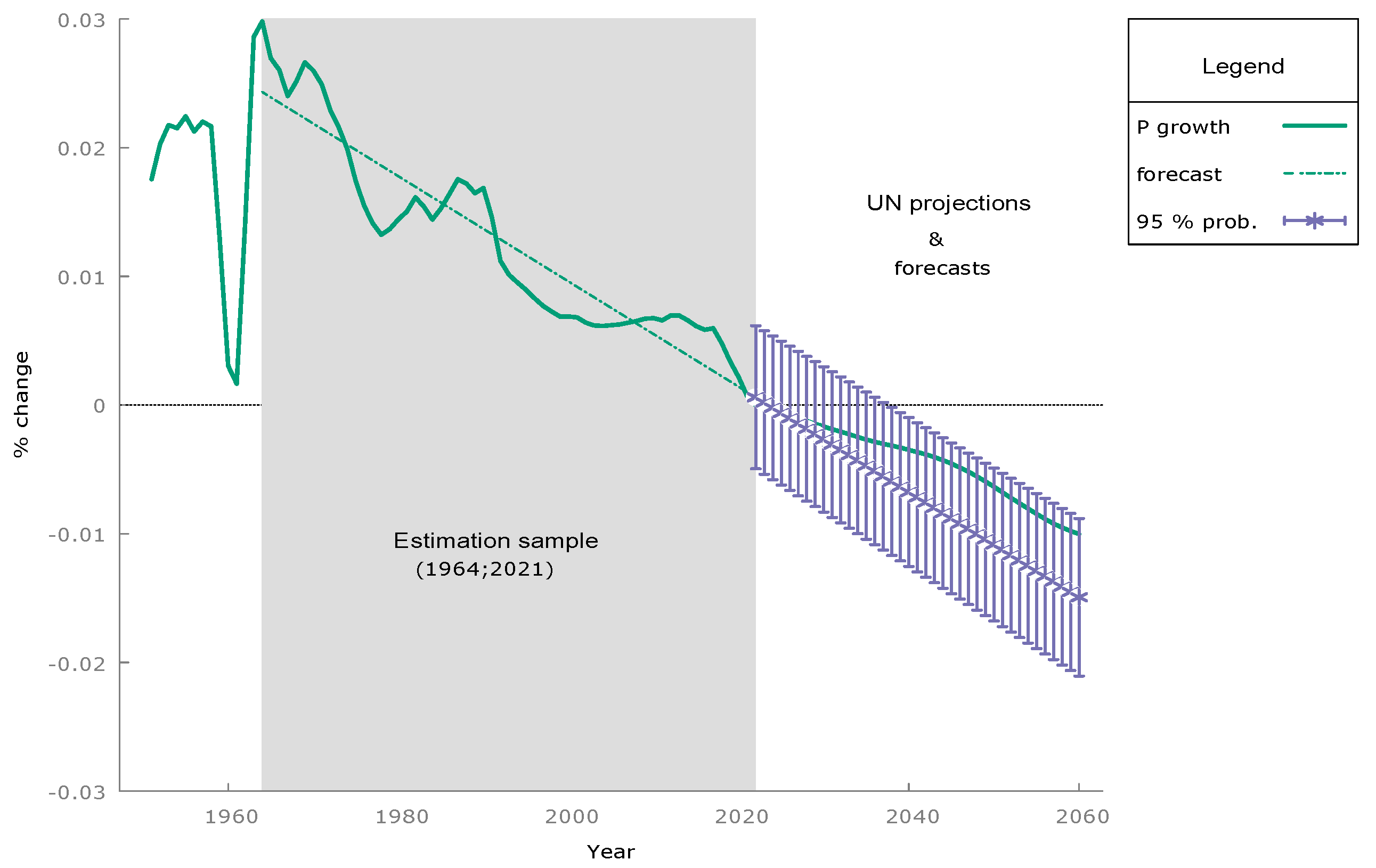
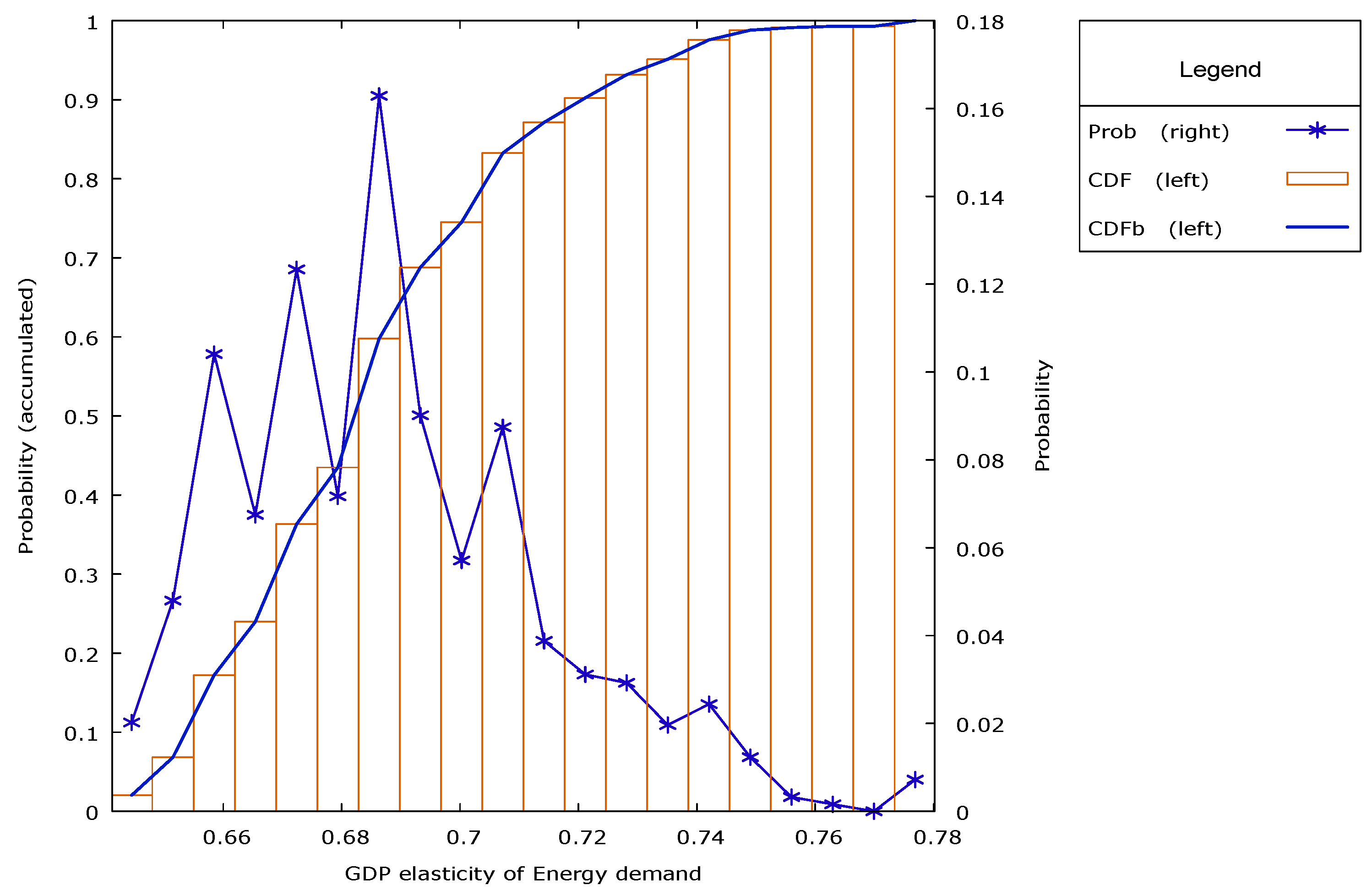
Project future energy demand up to 2060 and its full statistical distribution, going beyond the usual sensitivity analysis based on scenarios, which also allows for a risk assessment.

(3)

Evaluate the feasibility of achieving the neutrality objectives for the year 2060, presenting the discussion on the forecasts obtained independently, and without incorporating any assumption from the start that implies compliance with the objectives—as has been the usual practice in studies so far.

The reporting of this study is as follows: Starting from a survey of the most relevant contributions in this field carried out in Section 1, the general lines of the methodology are presented in Section 2. The series used, and the main results, are presented divided into several subsections in Section 3. Section 4 compares these results with the official projections and evaluates their feasibility. Section 5, finally, presents a brief summary of the conclusions and policy implications, as well as possible limitations and further extensions of the study.

2. Methodology

In a previous study [18], economic behavioral models were specified for the variables also considered in this new study, i.e., final energy demand, GDP growth, and population—although for a different economy, i.e., the aggregate world. The basic models analyzed here are inspired by those previous models, although the specification is different since the data and the case analyzed are also different. The method of analysis, however, is different and novel in the literature. The proposed methodology could be characterized, in a nutshell, as a robust estimate of the equilibrium trends, based on random samples over the selected historical period, which allows for obtaining a statistical distribution of the forecasts in the horizon of interest, the year 2060 in this case.

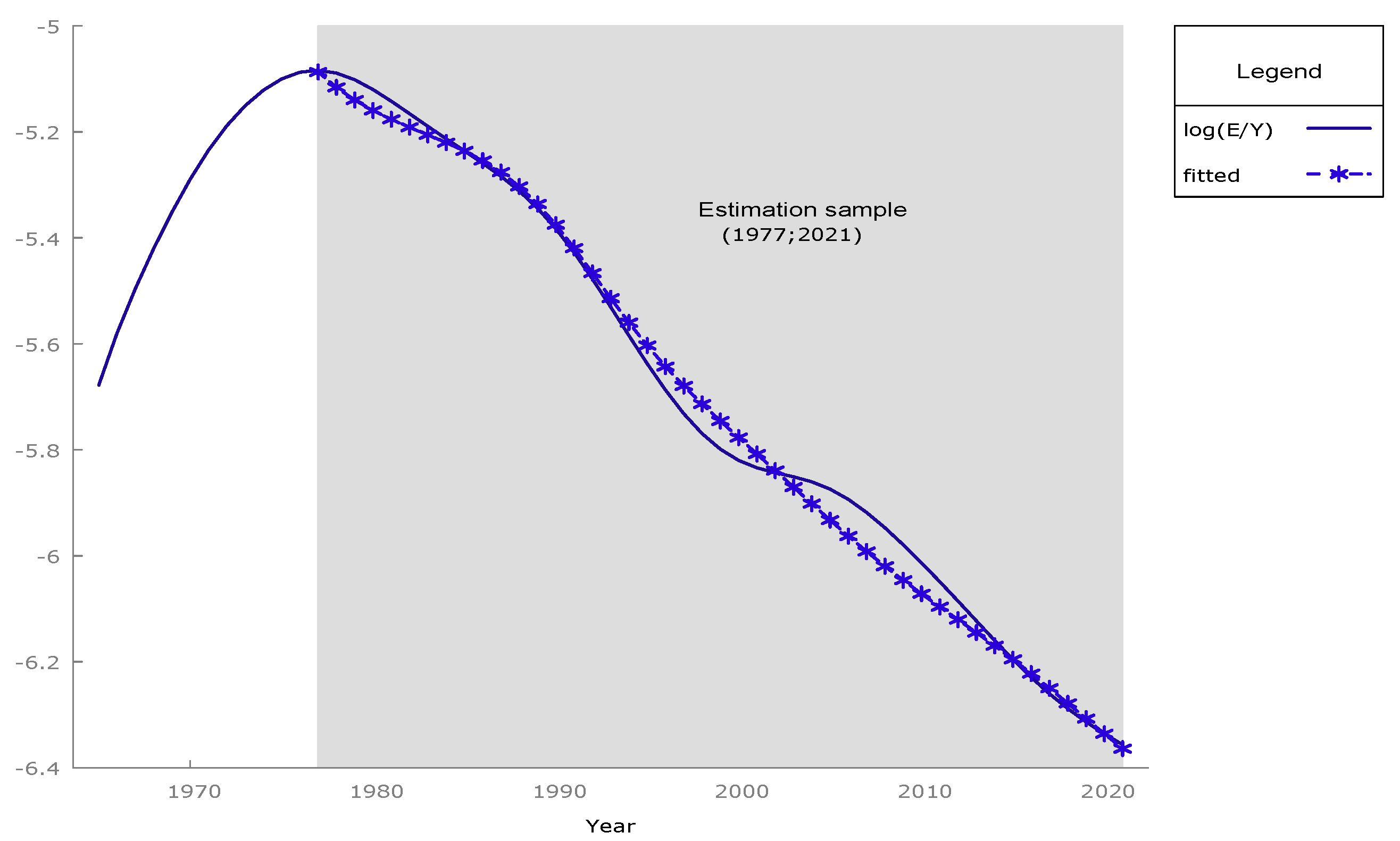
The first step is the estimation of the trends of the variables involved, conducted with a methodology based on the state space model [19]. It can be characterized as follows:

$$x_n=F{x}_{n-1}+G{v}_n$$

$$y_n=H{x}_n+w_n$$

(1)

where F and G are square matrices and H is a matrix of appropriate dimensions. The errors $v_n,w_n$ are white noise following the distributions of $N\left(0,{\tau }^2\right)$ and N$\left(0,{\sigma }^2\right)$, respectively. The model and the underlying variable $x_t$, i.e., the trend in this case, can be estimated by maximizing the likelihood and selecting the best degree of the dynamic model according to the Akaike Information Criteria (AIC). Analyzing the trends, rather than the original variables, has several advantages. First, this procedure removes random components that might overshadow the relationship among the variables analyzed. In fact, it is found that when estimating the models with the trend variables instead of the original ones, the precision of the estimates is greater, and their variance is lower. Additionally, it is sensible to assume that economic agents plan their future behavior considering a horizon, instead of simply reacting to contemporary changes. For this reason, it is likely that the estimation of the model with trend variables is more precise—in fact, it is easy to verify that, in this case, if it is estimated with observed variables instead of trend variables, then the estimators will be biased. However, in the event that economic agents decide their behavior based on the current values of the relevant variables without making future plans, the estimation of the model with trend variables is unbiased.

The second aspect to consider is the estimation method. In this study, the least absolute deviations (LAD) method [20] was chosen based on the minimization of Laplace errors. This method, as opposed to the standard method of ordinary least squares, is more robust, that is, less sensitive to possible outliers and erratic changes in short-term trends. All these phenomena almost certainly occur over a long historical period, such as the one considered here. Therefore, a robust method is preferable to the traditional least squares method. The LAD estimator is derived by minimizing the following expression with respect to (w.r.t.) the parameter vector $\beta$, over a set of T available observations,

$$min\left\{\sum _{t=1}^T\left|y_t-x_t^{\prime }\beta \right|\right\}$$

(2)

where $x_t^{\prime }$ is a vector of potential explanatory variables for the dependent observation, $y_t$. It is costlier to compute than the standard ordinary least squares estimator, but with the vast increases in computer power, this issue has become broadly irrelevant.

The next aspect is the estimate itself. First, the long-run equilibrium relationships are estimated, which can be estimated by directly relating the relevant variables in levels [21]. This avoids dynamic complications, which are only relevant in short-term forecasting. The linear dynamic model, which is standard in applied statistic research, can be written as follows:

$$∆y_t=∆\alpha \left(L\right)x_t^{\prime }-\gamma \left(y_{t-1}-{\beta }^{\prime }{x}_{t-1}\right)$$

(3)

where $\alpha \left(L\right)$ is a polynomial in the lag operator, L. The crucial insight is that the long-run equilibrium relationship, $\left(y_{t-1}-{\beta }^{\prime }{x}_{t-1}\right),$ can be estimated by directly omitting the dynamics—provided the variables are trending, and the fitted residual is stationary [21]. This estimation procedure is not appropriate for short-term forecasting, but is especially adequate when the objective is to derive long-run equilibrium forecasts. Furthermore, the estimation of simultaneous dynamic models can generate unstable dynamics that would invalidate the estimation process [22]. There is no clear method in the literature to avoid this problem, which makes it advisable to opt for the estimation of equilibrium trends, as is done in this study. The proposed method is inspired by the jackknife and bootstrap methods [23], in the sense that it is based on random selections from the sample under study, to set up the estimation sample in each case—i.e., for example, from a sample of T observations, T estimation samples are selected, dropping in each case a different observation. In addition, the size of the estimation sample is another variable to consider. This all generates a wide range of cases, which confirms the variability of the parameters throughout the historical period analyzed, and even that of the proposed model, since the statistical significance of the variables depends on the estimation sample. This variety of estimations, moreover, results in a non-trivial statistical distribution for the variables considered in the relevant horizon—the year 2060 in this case-, as well as for all intermediate dates. It must be emphasized that this method avoids and overcomes the traditional approach-scenario-based sensitivity test by supplying the complete statistical distribution of the simulated variable.

In summary, the procedure is based on the following points:

(a)

Extraction of the trends of the variables analyzed;

(b)

Identification of the essential characteristics of the variables, and of the general model;

(c)

Estimation of equilibrium trend relationships;

(d)

Application of the robust estimation method, LAD;

(e)

Selection of multiple samples, within the available database, randomly, and of different sizes;

(f)

Simulation and derivation of the future statistical distribution of the variables analyzed—notably energy demand, in the present case;

(g)

Characterization of the distribution obtained and risk analysis.

There are alternative simulation methods for future horizons. For example, bottom-up methods try to specify fairly detailed individual behavior relationships, and from there derive the future simulation—see, e.g., [18], for a more detailed discussion. The problem with these models, although they are theoretically superior, is that they require a large amount of data that are not available, so that in the end most parameters have to be inferred on a priori grounds. Disaggregated historical methods are also interesting, and are related to the method of historical series analysis proposed here. But the problem, again, is that the series are either not available or are too short to generate credible forecasts. Lastly, machine-learning and artificial intelligence methods, very popular in short-term forecasting, have proven their usefulness because they are capable of capturing highly non-linear relationships, which are impossible to detect with traditional statistical models. However, their ability to predict the long term is not entirely clear, since dynamic non-linear relationships, beyond a few observations very close to the estimation sample, can generate chaotic results, i.e., highly extreme and variable outcomes, because of their underlying mathematical properties [24].

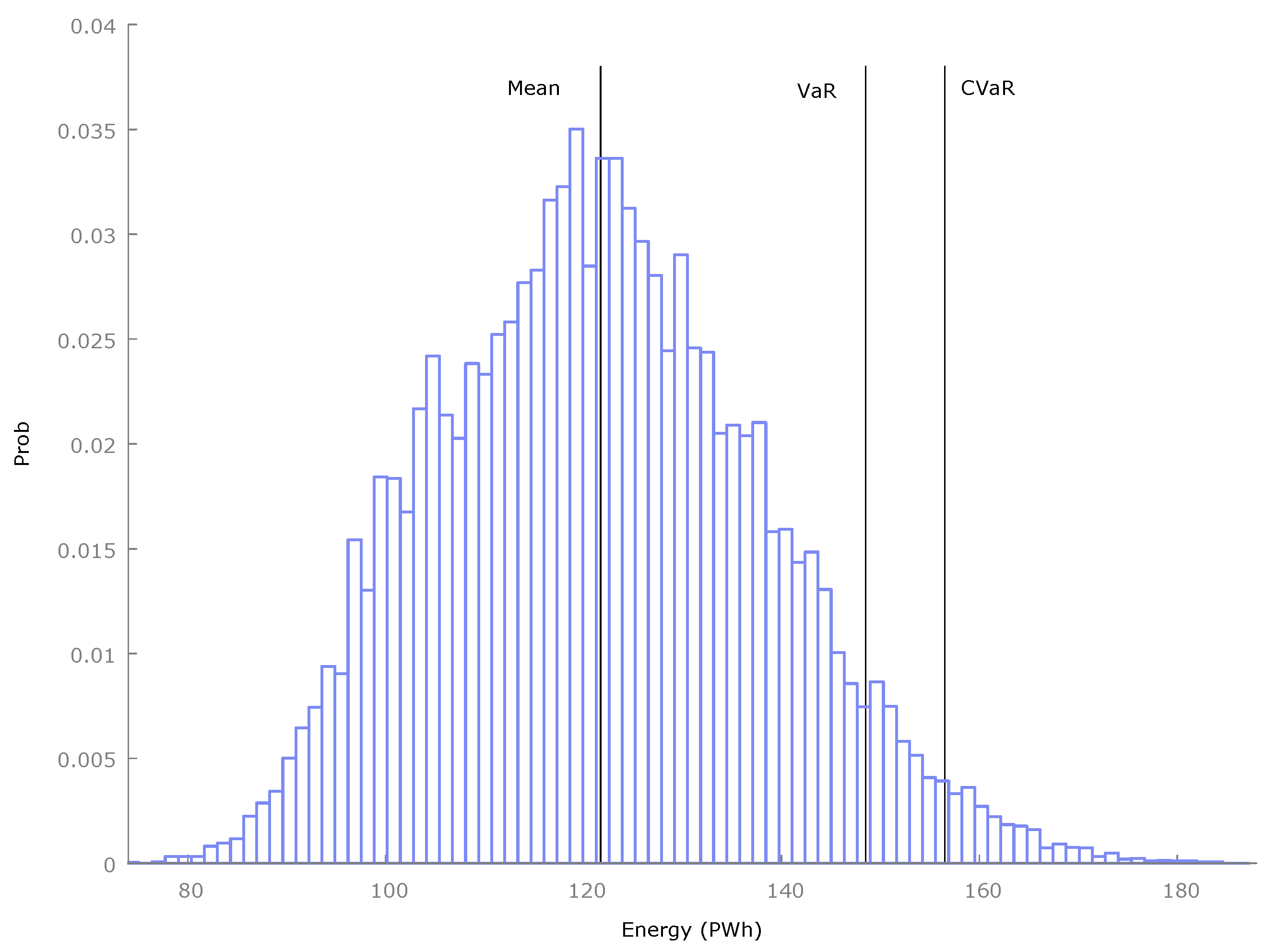
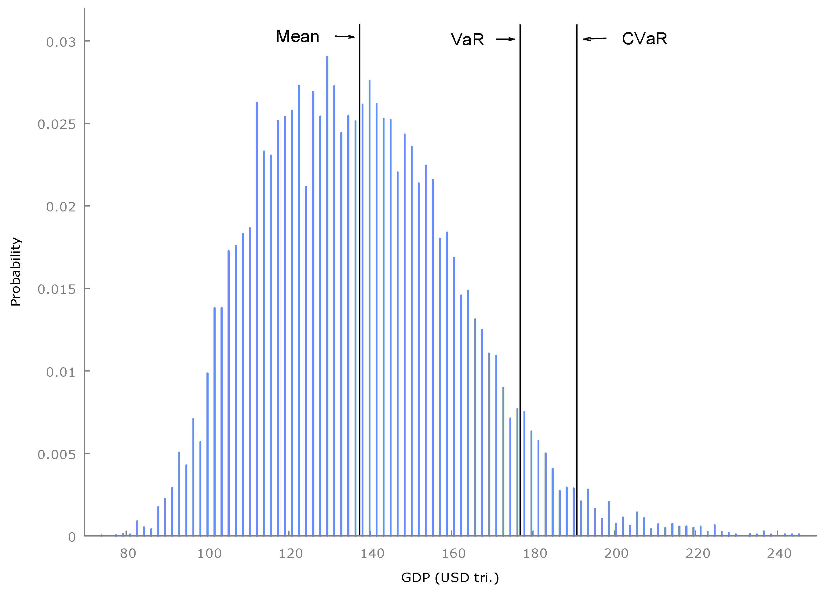
The next methodological aspect that is used in this work is the risk analysis, which is implied in the random distribution of the simulations. For this purpose, measures already known are used, such as the Value at Risk (VaR) and the Conditional Value at Risk CVaR, put forward and discussed by [25]. They are defined as follows,

$$Prob\left\{x\ge VaR\right\}=\alpha$$

$$CVaR=E\left\{x\left|x\ge VaR\right.\right\}$$

(4)

Fundamentally, these measures try to quantify the possibility, or likelihood, that an unfavorable event, even if not likely, will occur. These measures are calculated and presented in Section 3.

3. Empirical Results

This section reports the main results of the study. It is based on a dataset drawn from reliable international sources. Primary energy data since 1965 are available in terms of annual TWh in Our World in Data (OWD) [26]. Gross domestic product (GDP) data since 1950 are available from the Madison project [27], and for more recent dates, from the World Bank. Finally, regarding population data, they are available from 1820 in [27], and from 1950, including projections up to 2060, from the demographic department of the United Nations [28].

This section is organized as follows: Firstly, the main results of the trend analysis are presented in Section 3.1. Secondly, the more salient characteristics of the analyzed variables are analyzed in Section 3.2. Finally, Section 3.3 reports the results of the stochastic simulations up to the horizon of 2060.

3.1. Trend Analysis

Figure 1 displays the implementation of the trend estimation methodology discussed in Section 2 to the final energy demand. As can be seen, the trend smooths out a large part of the short-term random movements of the original observations and allows a better assessment of its long-term behavior.

The application of this methodology to the analysis of GDP and the population yields similar results, although in both cases the effect is not as pronounced, and therefore the corresponding figures are omitted.

3.2. Data Analysis

A preliminary analysis and description of the series can help to identify their main characteristics and the relevant estimation periods. First, the relationship between energy and income shows considerable increases in efficiency over time, as can be seen in the figure that displays this ratio—i.e., energy over GDP. Figure 2 displays the evolution of the logarithm of this ratio and a simple adjustment based on the logarithm of GDP. The final result is an elasticity that lies between 0.6 and 0.7 depending on the selected sample. Likewise, it can be checked that this relationship is relatively stable from 1977 onwards, which will be the period selected for the estimation. The population rate of change also turns out to be significant with a positive effect on the energy demand.

The analysis of the population is reported in Figure 3. Disregarding a highly variable behavior around 1960, the evolution of the population growth rate follows a clearly downward trend, which is sustained over the time period observed. In fact, a simple linear projection reasonably fits the observations and agrees, to some extent, with the predictions of the United Nations demographic department up to 2060 [28].

Finally, the evolution of GDP is analyzed in Figure 4. Two periods are clearly observed, before and after 2004, with considerable variability, especially before 2004. It is not possible to set up a model for the entire sample, nor for the period after 2004, since a simple trend would generate increasingly negative growth rates, something highly unlikely. Therefore, for this variable, the official expected values will be used to carry out the simulations. Nevertheless, to conduct stochastic simulations, the variability of this variable will be taken into account as follows: For the sample selected in each case, the mean and the corresponding errors will be estimated. These errors will be used to bootstrap the distribution and possible values of the variable—i.e., the GDP. More formally, given a subsample of size n derived by randomly selecting, without replacement, observations from the total available sample, T, the mean and the errors of the GDP are given by

$${GDP}_i=\widehat{m}+{\widehat{e}}_i$$

(5)

where $\widehat{m}$ is the estimated mean, ${\widehat{e}}_i$ is the fitted error, and $\left\{i=1,\dots ,n\right\}$. Simulated values for GDP are now derived by sampling from the estimated values, ${\widehat{e}}_i$.

Testing the validity of these relationships, mainly for energy demand, their eventual non-linearity is especially considered. To analyze this issue, the Loess [29] and the Nadaraya–Watson [30] non-parametric estimators are tested. Likewise, the quantile regression is also estimated [31]. In none of the three cases is a significant non-linear relationship detected—if the model is indeed non-linear, then the elasticity will vary according to different values of the explanatory variable, i.e., the GDP, as can be easily checked by means of a straightforward second-order Taylor expansion. However, what is observed is that depending on the samples, the elasticity changes, even if only within a reasonably limited interval. This variability of the model parameters has customarily been treated as a heteroskedasticity problem [32], but in this case, this approach is not suitable because a proper statistical test does not significantly detect it. Consequently, the estimation in different samples will result in a variable elasticity, and therefore a variable energy forecast, which will be taken into account in the random simulations of the scenarios analyzed up to 2060.

3.3. Stochastic Simulations

This subsection is devoted to reporting the main conclusions of the empirical findings of this study. The simulations are carried out by randomly selecting samples—repeatedly and of different sizes—within the historical period given by the database analyzed. More specifically, the estimation sample sizes run from 16 to 40 observations out of the available sample of 57 annual data. The number of draws in each case is directly related to the sample size. Finally, the model is simulated by generating 100 replications of the GDP as detailed in Equation (5). The total number of simulations is over 3 × 10⁵, which is taken as a sufficiently adequate number to capture and estimate the future distribution of the simulated variables, i.e., energy and GDP. Simulations with a lower number of observations, e.g., half, generated a similar histogram for 2060. The estimated equations are discussed in Section 3.2, and the GDP values are taken according to the official forecasts [5].

The fundamental reason for applying this methodology is that it allows for obtaining the random properties of a simulation, which is superior to a simple scenario model, and it is also justified by the variability of the parameter estimation in the selected historical sample. This can be checked graphically in Figure 5, where the different values of the GDP elasticity of energy demand are displayed according to the estimating sample. The figure presents the histogram and its accumulated values for the values obtained of the different elasticity estimates. Although the mean value is approximately 0.7, the variability is considerable, ranging between 0.66 and 0.78. This variability translates into the variability of the final distribution for the model simulations, especially energy and GDP.

The main results of the simulations are reported in

Table 1. Primary Energy Demand (PWh): Stochastic simulations.

	2030	2050	2060
mean	55.0	93.3	121.7
median	55.0	93.2	121.2
VaR	59.3	109.2	149.0
CVaR	60.4	113.8	156.6
CVaR (median)	60.1	112.6	155.0

. The table presents data for primary energy demand in PWh. It can be seen that, in principle, the distribution is quite symmetrical, since the mean and median are very close. However, the variability is considerable, as shown by the risk measures, in particular the CVaR. According to this measure, the energy demand could be nearly 30% higher than the average, although with not too high a probability of 5%. In any case, this measure provides an idea of the existing risk, and advises planning the deployment of renewable energy above the objectives set for the average, i.e., the mean value.

The following

Table 2. Gross Domestic Product (trillions): Stochastic simulations.

	2030	2050	2060
mean	36.6	88.2	137.4
median	36.5	87.7	135.7
VaR	40.0	107.6	177.0
CVaR	41.0	114.2	190.8
CVaR (median)	40.7	112.0	185.9

Notes: trillions USD international PPP constant 2017 prices.

presents the results of the GDP simulations. In this case, the variability is greater, and in fact, when comparing the CVaR with the mean, it turns out to be almost 40% larger. These simulations are based on the official projections for GDP, but since its wide variability over the period considered is implemented into the simulations—see Figure 4—the possible final values lie within a fairly wide range.

Figure 6 and Figure 7, finally, visually report the results obtained and presented in the previous tables. Figure 6 displays the histogram of the simulations for energy, in this case in TWh. The histogram is reasonably symmetrical, as noted above, given the similarity between the mean and the median, although the risk measures reveal a right tail quite far from the mean; indeed, some values are rather extreme, e.g., 180 PWh, even if with a low probability.

The histogram for GDP is presented in Figure 7 and the comments are similar. In this case, the symmetry is less marked, even if the similarity between the values of the mean and median may suggest otherwise. It should be emphasized that the simulations are based on official projections, although the great variability observed is due to the simulated errors obtained from the adjustment of the mean in each selected estimation sample.

These results can be compared with those derived by means of a standard simulation of the estimated energy demand model over the whole sample $\left(t=1,\dots ,T\right)$, i.e.,

$$\alpha \left(L\right)log\left(E_t\right)={\beta }_0+{\beta }_1\left(L\right)log\left({GDP}_t\right)+{\beta }_2\left(L\right)∆log\left({Pop}_t\right)+{\epsilon }_t$$

(6)

Simulating this equation up to 2060, conditional on the official forecasts for GDP and the population projections of the UN [28], yield 142.5 trillion USD for GDP and 125.5 PWh for primary energy. These values are somewhat larger than those reported in Table 1 and Table 2. Additionally, the stochastic distribution of the simulations can only be derived under strong further assumptions on the specified model.

The significance of these results and their implications are analyzed in the following Section 4.

4. Discussion

In 2020 the Chinese government announced a pledge to become carbon neutral by 2060. Later, specific roadmaps were presented by several official institutions—e.g., [5,6,7]. To do this, firstly, energy demand projections were used in all the corresponding years from the present, up to and including 2060. Therefore, it is adequate now to compare these official forecasts with the results in the empirical Section 3. The Chinese plans considered three possible scenarios [7], and

Table 3. China 2060 Green Urgent Scenario (GUS).

	2020	2060
Fossil sources	426.5	86.7
(%)	85.1	15.1
Renewable sources	74.7	487.2
(%)	14.9	84.9
Total	501.2	573.9

Notes: Units—10 b. tons of standard coal.

presents one of them, the most ambitious in the sense that it implies a greater share of renewable energy—see

Table A1. Primary Energy Demand Forecast—Green Urgent Scenario (GUS).

	2030	2040	2050	2060
Coal	276,584	180,939	86,036	17,143
Oil	104,274	87,060	58,360	28,572
Natural gas	69,021	81,861	75,772	41,230
Hydropower	50,150	53,768	56,481	62,160
Nuclear Power	21,240	35,178	52,547	77,700
Wind Power	42,185	77,220	115,210	152,810
Photovoltaic	38,055	78,936	123,640	168,350
RE (other)	236	1716	7025	25,900
Total	601,745	596,679	575,071	573,865

Notes: Units—10 thousand tons of standard coal. Source, [7].

in Appendix B for more detail on the specific roadmap over the years and a breakdown of energy types. A forecast of the CO₂ emissions pathway compatible with the 1.5 °C target, broadly in line with the Green Urgent Scenario analyzed next, is also reported in Appendix B,

Table A2. CO₂ emissions under the 1.5 °C scenario.

2020	2030	2050	2060
10.03	7.44	1.47	0

Units: tce (metric tons of coal equivalent). Source, [5].

.

Although the units used by Chinese official statistics are different from the usual ones in international organizations, it can immediately be seen that the increase in primary energy from 2020 to 2060 is approximately 14%—(573.9⁄501.2) − 1≅14%. This contrasts sharply with the values obtained in the results of the empirical section, where an increase close to 200% in primary energy demand was forecast between those years. The aim of this section is to discuss whether this large discrepancy can be covered, and therefore whether the official Chinese plans are achievable.

First, it should be underlined that the predictions of the empirical Section 3.3 refer to primary energy, but a conversion to final energy has to be implemented because fossil fuels lose a large amount of potential energy in combustion processes, energy that is not recoverable, in general. It is just the opposite with RE, since their power is immediately converted to electricity, and therefore the losses are minimal. The conversion factors from primary to final energy are debatable, but those most accepted by international organizations such as Irena [33], the IEA [34], and the European Union [35] range between 50% and 60%. With these values, and taking into account that the proportion of RE in the plan analyzed in Table 3 is approximately 85%, the final energy (FE) involved in this plan, according to the forecasts of the empirical results, would be the following:

$$FE<-121\times 0.85\times 0.55+121\times 0.15=74.717$$

(7)

The final simulated primary energy, on average, for 2060 in Table 1 is 121 PWh. The result obtained, therefore, is approximately 75 PWh. To assess this value, we can apply the 14% increase in energy assumed in the plan in Table 3 to the energy effectively consumed in 2020, which generates approximately 47 PWh. Subtracting this figure from the previous forecast, i.e., 75 PWh, yields the following value: 74.717 PWh − 47.310 PWh = 27.407 PWh. This figure implies an excess demand of approximately 50% over the planned energy.

The question now is whether this energy demand excess can be explained away by savings and other increased efficiency measures. In order to discuss this issue, a study focusing on the whole world conducted by [36] can be brought to bear. In that study, the authors consider a series of efficiency and savings measures that can be classified into three broad categories: (a) changes in dietary and transportation patterns, (b) deployment of renewables with an increase in the participation of prosumers, and (c) efficiency gains in buildings and telecommunications. With these three types of measures, the authors conclude that an additional 40% could be saved in energy demand. Applying this reduction to the previously obtained figure of 74.7 PWh yields a final value of 44.8 PWh, which is already lower than the forecast value of 47.3 PWh. Therefore, assuming that these savings and efficiency gains can be realized, the plan in Table 3 put forward by the Chinese government would be feasible.

Nevertheless, a set of caveats should be underlined in this regard. First, the savings assumed in [36] include the deployment of RE, something that is already considered in the first transformation that has been carried out in this section to reach the figure of 74.7 PWh. Secondly, this plan includes significant changes in demand patterns, in particular in diet and transport, something that would require a change in the preferences of consumers, or at least a change in the transport infrastructures so that it would be possible to replace private with public transportation. Thirdly, the plan assumes a very rapid and accelerated deployment of RE, although taking into account the previous performance of the Chinese economy, it could be surmised that this would be the least problematic aspect. Fourthly and lastly, it should be noted that in this analysis we start from a forecast of average demand, but this forecast is random and, in fact, there is a non-negligible probability that the final demand turns out to be much higher, as pointed out in Table 1 in the empirical Section 3.3. Therefore, the recommendation would be to plan for a demand that could be significantly higher to guarantee that the objectives of a carbon-neutral economy are achieved.

As a summary, possibly the main issue to be remarked on is that it will be necessary to change the habits and consumption patterns of society in order to achieve the decarbonization objectives. This may seem hazardous from a political point of view, but in this regard, it is interesting to note the research by [37], where they show that many of the changes in demand required to reduce carbon emissions would actually improve the utility of individuals.

Although the main conclusion obtained in this study as an answer to the initial research question, i.e., the feasibility of the objective of carbon neutrality in 2060, is affirmative and similar to that of other academic studies [9,10,11,12], the methodology is very different. First, those studies are based on short annual series—i.e., a maximum of 20 years, compared to the 57 used here. Additionally, the aforementioned studies embody the assumptions of efficiency [9] or a reduction in emissions [11] in the forecast model in one way or another. The approach followed here, on the contrary, consists of an estimate and projection of the expected demand in an independent way, and only from there has this conclusion been reached, analyzing the necessary expansion of RE and the necessary savings in the consumption of energy and lifestyle changes. The study by [13] is based on a different quantitative methodology, and although it expresses certain doubts regarding the feasibility of the neutrality target for 2060, it only goes until 2026. The study by [16], on the other hand, although not directly addressing the projection of energy demand, is relevant and complementary to all the others, including this study, to the extent that it stresses the critical need for rare minerals.

5. Conclusions

The purpose of this study is to estimate China’s primary energy demand in 2060, and to assess the feasibility of achieving the carbon neutrality objectives announced by the Chinese Government. To this end, a primary energy demand model is estimated using a novel method, which allows for obtaining the statistical distribution of demand in 2060. This, in turn, allows for carrying out a complete risk analysis, due to the uncertainty involved in the random distribution, and overcoming the standard sensitivity analysis based on scenarios. Second, the modeling is based on long historical series from reliable international sources. The first conclusion obtained is that the expected energy demand, in principle, is much higher than that officially forecast by China. However, taking into account renewable energy expansion plans of up to 85%, this discrepancy is reduced to only 50% higher than the official forecast. If feasible savings and efficiency gains based mainly on changes in transportation patterns and dietary styles according to international research are added, then this excess could be further shrunk by almost an additional 40%. The final result of these calculations is that the expected primary energy demand, on average, could be within the range of the official forecasts. Nevertheless, this refers to the average value, and there is a small but non-negligible probability—specifically 5%—that the final demand is up to 30% higher than the expected average demand. Several conclusions can be drawn from this analysis: Firstly, to achieve this objective, a strong and unwavering political commitment is necessary, aimed at accelerating the renewable transformation, as well as modifying behavior patterns, especially with regard to transport and dietary habits. Furthermore, since these conclusions refer only to average values, the speed of RE deployment must be even greater if the risk of excess demand is to be reduced. The intensity and magnitude of the effort required to achieve this objective demands several additional aspects, as also pointed out both in the official Chinese plans and by international organizations—e.g., the IEA and Irena.

The risks implied by current international events cannot be overemphasized either. Specifically, the Ukraine war underlines the need to achieve energy independence, and given the lack of one’s own fossil resources, points to accelerated RE deployment as the only way out. The social pressure to recover the pre-pandemic growth levels is also another significant risk, inasmuch as it may lead to choosing the easiest short-term way out, namely, increasing coal-related developments [38].

From the sustainable development goals perspective, the Chinese stance underscores the transition from simply material growth at any rate to quality growth focused on the wellbeing of the people and the environment. This may also set a policy example for other countries. Specifically for other developing countries, several lessons are immediate from these results: first, the need to accelerate the deployment of RE and to avoid all kinds of short-run pressures to continue consuming fossil resources; second, to ensure energy security, fossil fuel dependence must be curtailed as fast as possible; third, the focus on quality growth rather than straightforward material growth, coupled with dietary and demand consumption changes.

Regarding the limitations of this study, perhaps the main one also derives from its advantages, which is the use of long, but highly aggregated historical series. Thus, possibly the most promising extension of this study would consist of combining the long historical series used here with disaggregated series, e.g., by type of energy or by province, but much shorter, as those used by other researchers. Combining both sources of information would make it possible to obtain more reliable results, although the methodology to do so is only available to a limited extent. Another aspect to develop is the estimation of alternative, and specifically dynamic, models instead of the equilibrium approach adopted here. This approach can imply instabilities, but if they are resolved then it could offer a point of contrast to the results presented here. Finally, the estimation method and the methodology for the selection of the samples is another point that deserves to be developed.

All these aspects open a new line of research that would also allow the implementation of this newly presented methodology to other regions and countries.