Article

Energy Performance of Room Air-Conditioners and Ceiling Fans in Mixed-Mode Buildings

1
Energy Policy, Wuppertal Institute for Climate, Environment and Energy, 42103 Wuppertal, Germany
2
E3D—Institute of Energy Efficiency and Sustainable Building, RWTH Aachen University, 52062 Aachen, Germany
3
Centre for Advanced Research in Building Science and Energy (CARBSE), CEPT University, Ahmedabad 380009, India
*
Author to whom correspondence should be addressed.
Energies 2023, 16(19), 6807; https://doi.org/10.3390/en16196807
Submission received: 11 August 2023 / Revised: 1 September 2023 / Accepted: 12 September 2023 / Published: 25 September 2023
(This article belongs to the Topic Building Energy Efficiency)

Abstract

:
Studies show that people can tolerate elevated temperatures in the presence of appreciable air movement (e.g., from using ceiling fans). This minimises the use of air-conditioners and extends their set-point temperature ( T s e t ), resulting in energy savings in space cooling. However, there is little empirical evidence on the energy savings from using ceiling fans with Room Air-Conditioners (RACs). To address this gap, we analysed the energy performance of RACs with both fixed-speed compressors and inverter technology at different set-point temperatures and ceiling fan speed settings in 15 residential Mixed-Mode Buildings (MMBs) in India. Thermal comfort conditions (as predicted by the Indian Model for Adaptive Comfort-Residential (IMAC-R)) with minimum energy consumption were maintained at a set-point temperature ( T s e t ) of 28 and 30 C and a fan speed setting of one. Compared with a T s e t of 24 ° C, a T s e t of 28 and 30 ° C resulted in energy savings of 44 and 67%, respectively. With the use of RACs, a configuration with a minimum fan speed was satisfactory for an optimal use of energy and for maintaining the conditions of thermal comfort. In addition, RACs with inverter technology used 34–68% less energy than fixed-speed compressors. With the rising use of RACs, particularly in tropical regions, the study’s outcomes offer a significant potential for reducing space-cooling energy consumption and the resultant greenhouse gas (GHG) emissions.

1. Introduction

1.1. Overview

Since 2000, global energy demand for space cooling has increased by an average of about 4% per year, resulting in significant greenhouse gas (GHG) emissions [1]. Most residences and small offices in tropical countries such as India operate as MMBs, i.e., they operate in a fully air-conditioned mode or with natural ventilation (through operable windows) depending on the weather conditions. They switch between the modes according to the seasons or even within a day. Typically, natural ventilation through manually operable windows and the use of ceiling fans for local air movement are popular strategies to achieve thermal comfort satisfaction [2,3,4]. India’s climate makes space cooling a significant electricity end use in buildings [5]. RACs are used for air-conditioning in residences and their market penetration and usage has been increasing. This also leads to an increase in energy consumption and GHG emissions, which need to be reduced while ensuring that people’s aspirations and thermal comfort needs are met. In India, the Minimum Efficiency Performance Standards (MEPS) for RACs (with compressors of fixed speed and inverter technology) and ceiling fans are governed by the Bureau of Energy Efficiency (BEE)’s Standards and Labellings (S&Ls) programme to increase their energy efficiency [6]. Alongside such MEPS programmes, optimising their use is essential to minimise space-cooling energy consumption.
Studies show that people tolerate elevated temperatures in the presence of appreciable air movement (see Section 1.2), which reduces energy consumption for space-cooling (see Section 1.3). In India, most buildings with Room Air-Conditioners (RACs) and ceiling fans operate as Mixed-Mode Buildings (MMBs). RACs are only used when thermal comfort conditions cannot be maintained through natural ventilation or ceiling fan usage (see Section 1.4). However, the extent of energy savings through the use of ceiling fans with RACs in Indian MMBs is unclear (see Section 1.5). Therefore, this study analysed the energy performance of RACs and ceiling fans in relation to the indoor conditions and thermal comfort as predicted by the Indian Model for Adaptive Comfort-Residential (IMAC-R) [7]) (see Section 1.6). In addition, RAC usage behaviour and the energy performance of RACs with inverter technology and fixed-speed compressors were analysed.

1.2. Tolerating Elevated Temperatures with Appreciable Air Speed

In warm and hot climates, the movement of air close to the skin increases the evaporation of perspiration, reduces heat stress and helps to achieve thermal comfort satisfaction [8,9,10]. Studies show that occupants are able to tolerate elevated temperatures in the presence of adequate air velocity [11,12,13]. In a comprehensive review of fan use in field studies, Ref. [14] found that fan use increased the average neutral comfort temperature by up to 3 ° C without affecting productivity. Ref. [15] observed that the Tropical Summer Index (TSI), a measure of thermal comfort for Indian subjects based on laboratory experiments, could vary by up to 3.2 ° C with an indoor air velocity ( v e l ) of up to 2.5 m/s. In thermal comfort studies in naturally-ventilated (NV) buildings across climate zones in India [16], observed that beyond an indoor operative temperature ( T o p ) of 22 ° C, the mean indoor indoor air velocity ( v e l ) increased with the mean indoor operative temperature ( T o p ), reaching a maximum of approximately 2 m/s at a T o p of 30 ° C. Similarly, in naturally-ventilated (NV) buildings (residential and commercial) in a composite (Composite climate experiences a combination of warm and humid, warm and dry, monsoon and cold periods.) climate zone in India, Ref. [17] observed that comfort temperature could be increased by up to 3 ° C when the ceiling fans were switched on. In MMBs and NV buildings in a composite climate zone in India, Ref. [18] found that the indoor operative temperature ( T o p ) for thermal comfort could be increased from 27 to 31 ° C when the indoor indoor air velocity ( v e l ) was increased by up to 1.5 m/s. To maintain thermal comfort conditions, the National Building Code (NBC) of India recommends an indoor indoor air velocity of up to a maximum of 3.2 m/s at an indoor operative temperature ( T o p ) of 35 ° C and relative humidity ( R H ) of 30% [19].

1.3. Space-Cooling Energy Savings with Fan Usage

As occupants tolerate elevated temperatures when presented with an acceptable air speed, the resultant energy savings are estimated in two ways.
  • By reducing the duration of RAC usage. That is, occupants are more likely to use ceiling fans than RACs if thermal comfort can be maintained only with fan usage, which consumes lesser energy. Based on a study of human thermal comfort in an environmental chamber [12] found that an increase in the indoor air velocity ( v e l ) between 0.5 and 1.0 m/s compensated for an increase in the indoor air temperature ( T i n ) from 2.8 to 3.3 ° C and could save 15–18% energy. The energy savings were calculated by using the estimate from the United States National Bureau of Standards (USNBS) that a 1 ° C increase in the set-point temperature ( T s e t ) results in 6% energy savings. Ref. [14] concluded that ceiling fans could reduce the use of air-conditioning by 15%. Ref. [20] estimated that space cooling consumption in Australia could be reduced by 76% by using fans with air speeds up to 1.2 m/s when compared with using RACs alone, based on the USNBS’s estimate.
  • By extending the set-point temperature ( T s e t ). This means that the occupants are more likely to use RACs with an extended set-point temperature ( T s e t ) when they are presented with an acceptable indoor air velocity ( v e l ). The use of RACs at an extended set-point temperature saves more energy than the additional energy consumption of the ceiling fan. In office spaces with RACs in Ghana, Ref. [21] estimated simulated energy savings from 8 to 33% and from 12 to 44%, respectively, by increasing the T s e t from 21 to 25 ° C during peak and from 22 to 26 ° C during low outdoor conditions. Compared to a static set-point temperature, an adaptive set-point temperature (i.e., T s e t based on adaptive thermal comfort models) reduces energy consumption because an adaptive set-point temperature is usually higher than a static set-point temperature, which is typically set between 22 and 24 ° C [22,23]. In a review, Ref. [24] found that most studies had reported an average energy savings from 6 to 10% per 1 ° C rise in the set-point temperature ( T s e t ).

1.4. Room Air-Conditioner and Ceiling Fan Usage in India

An analysis of residential electricity load studies conducted in various Indian states and cities indicated that air-conditioners, which included evaporative air coolers, and ceiling fans contributed significantly to the summer load [25,26,27]. Peak load levels were typically observed between 9:00 and 18:00 during the day and between midnight and 5:00 during the night. An in-depth analysis on the use of residential RACs by Ref. [26] found that households used RACs for an estimated 200 and 1200 h per year. According to a household survey conducted in Delhi, a city with a composite climate, Ref. [28] found that on a typical summer day, 30% of households used RACs for an average of five–six hours and 14% of households used RACs for more than eight hours. Few studies observe the energy consumption of RACs under different indoor conditions and in relation to user behaviour, apart from household electricity consumption surveys and household energy use studies. In one particular study, Ref. [29] analysed the behaviour of RAC users in eight residences in Hyderabad, a city with a composite climate. During a 30-day period, the authors analysed the metered energy consumption (of the residence) and the indoor conditions, specifically, the indoor air temperature ( T i n ) and the relative humidity ( R H ). In summer, users switched on the RACs at an indoor air temperature ( T i n ) from 29 to 31.9 ° C and an indoor relative humidity ( R H ) from 36 to 38.9%, and in monsoon, at an indoor air temperature ( T i n ) from 26 to 28.9 ° C and an indoor relative humidity ( R H ) from 59 to 61.9%.
In nonresidential buildings, in hot and dry climates, Ref. [16] found that fans were used consistently during the summer and monsoon seasons and were used less frequently in the winter. Moreover, in hot and humid climates, fans were used year-round. In composite and warm and humid climate zones, the use rate of fans in mixed-mode offices was observed to be 68% and 85%, respectively, by [30] when the outdoor daily mean temperature was 29 ° C. There are a limited number of published studies on the usage of ceiling fans in residential MMBs in India, and whether the ceiling fans are simultaneously used with RACs.

1.5. Research Gaps and Motivation

Energy savings from an extended set-point temperature ( T s e t ) are often calculated by applying the USNBS’s estimate to findings from studies on thermal comfort and simulated energy savings. Only a few studies have presented monitored energy savings. Empirical studies on the energy consumption of RACs and ceiling fans at different set-point temperatures ( T s e t ) and fan speed settings (FSSs) in relation to thermal comfort conditions and user behaviour are lacking. Therefore, the present study aims to fill this gap by conducting an empirical investigation on Indian buildings as an illustration. In particular, some research gaps are listed below.
  • The usage of RACs with ceiling fans, especially at high fan speed settings, may increase the convective heat transfer from the interiors. It is unclear whether the static or dynamic values for indoor-surface heat transfer coefficient h i assumed in simulated studies sufficiently represent the actual values [31]. Furthermore, heat dissipation may occur from fan motors. These factors can lead to an increase in the indoor air temperature ( T i n ). This increases the space cooling load and reduces the expected energy savings due to ceiling fan usage. A pilot study has provisionally shown that the use of ceiling fans with RACs could increase the indoor operative temperature ( T o p ) in Indian buildings [32].
  • The relationship between the set-point temperature ( T s e t ), indoor conditions and RAC energy consumption in Indian Mixed-Mode Buildings (MMBs) is unclear. The Bureau of Energy Efficiency (BEE) estimates that rising the set-point temperature ( T s e t ) in offices from a typical temperature of 20 ° C to 24 ° C will result in 23 billion units of electricity nationally by 2030. This is by applying the USNBS’s estimate [33]. However, studies show that an adaptive set-point temperature is sufficient to achieve comfortable indoor conditions as predicted by the Indian Model for Adaptive Comfort (IMAC) model and results in significant energy savings [34]. Moreover, as most people already prefer a T s e t of 24–26 ° C, as shown in a residential RAC survey by [28], the energy savings estimated by the BEE may be simplistic and unrealistic.
  • Most thermal comfort studies from India on the ability to tolerate elevated air temperatures in the presence of air velocity were conducted in naturally-ventilated buildings. Where RACs are available, it is uncertain whether the occupants actually tolerate the elevated air temperatures predicted by the thermal comfort studies prior to switching on the RACs. For example, people who can tolerate an indoor operative temperature ( T o p ) of 32 ° C may tend to switch on the RACs at a T o p of 30 ° C if the RACs are available. Without a corresponding increase in the set-point temperature ( T s e t ) (i.e., extended T s e t ), the use of ceiling fans results in additional energy consumption [35].

1.6. Objectives of the Study

This study empirically evaluated the impact of the simultaneous use of ceiling fans and Room Air-Conditioners (RACs) on space-cooling energy consumption and indoor thermal comfort conditions in Indian MMBs. We analysed the energy consumption of RACs and ceiling fans at various set-point temperatures ( T s e t ) and fan speed settings fan speed settings (FSSs), respectively, in relation to the IMAC-R adaptive thermal comfort model. Specifically, the study sought answers to the following questions.
  • What is the extent of energy savings when ceiling fans are used with Room Air-Conditioners (RACs)?
  • What is the extent of energy savings due to an extended set-point temperature ( T s e t )?

2. Materials and Methods

2.1. Location of the Study

The study was conducted in the bedrooms of 15 residential buildings in two Indian cities, Visakhapatnam and Hyderabad, with warm and humid and composite climates, respectively [19]. See Figure 1 for a representative image; some more pictures of the buildings and rooms are shown in Appendix B. All houses were constructed with a Reinforced Cement Concrete (RCC) framed structure with burnt brick masonry walls and an RCC roof. Typically, walls were constructed with 230 mm burnt brick masonry plastered on both sides with 12 mm cement plaster. In our samples, H1, H2 and H3, fly ash bricks were used. The U-value of walls ranged approximately from 1.8 to 3 W/m 2 K. Roofs were constructed with 150 mm RCC plastered on both sides with cement plaster, with a U-value of 3 W/m 2 K, approximately. Most of the new buildings had 12 mm plasterboard false ceilings, 150 mm from the ceiling. All houses had single-glazed windows with wooden, Unplasticised Polyvinyl Chloride (UPVC), or aluminium frames, with a U-value of approximately 5–5.5 W/m 2 K.
Each bedroom had an RAC and a ceiling fan. In total, there were eight popular brands of RACs and four popular brands of ceiling fans. The cooling capacities of the RACs were around 3350 W (usually marketed as 1 tonne of refrigerant (TR) RACs) and around 5440 W (1.5 TR). The ceiling fans had a diameter of 1200 mm, a rated power input of approximately 75 W, an air flow of between 210 and 240 m 3 /min (between 310 and 390 rotations per minute (RPM)) at full speed. There were superefficient ceiling fans with a rated power input of 28 W in two samples. Table 1 shows the physical characteristics of the bedrooms (floor area, floor-to-ceiling height and Window-to-Wall (area) Ratio (WWR)), specifications of the RACs (efficiency according to the Energy Efficiency Ratio (EER) or the Indian Seasonal Energy Efficiency Ratio (ISEER) (The EER gives the ratio of the cooling capacity (kW) of the RAC to its electrical power input (kW); “ISEER means the ratio of the total annual amount of heat that the equipment (kWh) may remove from the indoor air when operated for cooling in active mode to the total annual amount of energy consumed by the equipment (kWh) during the same period”; definitions and testing conditions for the EER and ISEER are given in the Gazette Notification by the [6]. The EER was replaced by the ISEER after 1 January 2018, capacity at full load (100%) and half load (50%), their star rating according to the S&L programme of the BEE and the labelling period, the furniture in the room and occupancy pattern.

2.2. Procedure of the Study

Most studies evaluate the energy savings of an extended set-point temperature ( T s e t ) by extrapolating the results of thermal comfort studies or simulation studies [24], as explained in Section 1.3 and Section 1.5. As there are few empirical studies on this subject, this study developed a novel approach to assess the effect of set-point temperature ( T s e t ) and fan speed settings (FSSs) on indoor conditions in real buildings. The study was conducted in Visakhapatnam from 25 April to 8 May 2022 and in Hyderabad from 12 to 28 May 2022. It consisted of two parts.
  • An experiment, primarily to analyse the indoor conditions and energy consumption due to changes in the set-point temperature ( T s e t ) and fan speed settings (FSSs).
  • An analysis of RAC user behaviour (limited to switching the RAC on and off) in relation to the indoor conditions.

2.2.1. Experiment

In each building, the study was conducted for 12 days. On each day, RACs were continuously run for five hours between 10:00:00 and 14:59:00 at a specified T s e t . On the first day, the T s e t was 20 ° C. On the second day, the T s e t was increased by 2 ° C to 22 ° C. In this way, T s e t was increased until it reached 30 ° C on day six. For the next six days (i.e., from days 7 to 12), the same set of T s e t was again repeated, except for minor differences in the order (see Table 2). This was done to mitigate the effect of unusual weather patterns on any given day, e.g., a particularly cloudy or rainy day.
Furthermore, each day, the ceiling fan speed setting was changed at every half hour, as shown in Table 3. During the experiment, most of the rooms were unoccupied, with the exception of V5 and H4, which were intermittently occupied by an adult and where a desktop computer was in use (see Table 1). Textile curtains were drawn over the windows and the doors were kept closed to maintain the typical conditions when people use RACs. For the analysis, data in Visakhapatnam and Hyderabad were considered from 10:30:00 to 14:59:00 and 10:00:00 to 14:29:00, respectively, to facilitate a comparison in both cities for the same set-point temperature ( T s e t ), fan speed settings (FSSs) and duration.

2.2.2. RAC User Behaviour Analysis

In six of the samples (V2, V5, V6, V7, H4 and H7), the rooms were occupied outside the experimental periods, mostly during the night for sleeping and sometimes in the evening. The activity level was mostly sedentary. The indoor conditions ( T i n and R H ) were analysed to observe the switch-on and switch-off behaviour of the RACs. The age, gender and number of occupants in the six samples were: V2—a male of 62 years and a female of 60 years; V5—a male of 22 years; V6—a female of 75 years; V7—a male of 70 years; H4—a male of 25 years; a male of 55 years. The insulation of the occupants’ clothing was not known, although blankets are usually used for sleeping, especially when RACs are used.

2.3. Instruments, Measurements and Data Collection

2.3.1. Instruments

We assembled eight sets of custom-built monitoring instruments to take continuous measurements during the study. Each set consisted of three modules as listed below. Each module had appropriate sensors/components connected to a Wemos D1 mini pro board based on the ESP-8266EX microchip, which is an Arduino-based Wi-Fi microcontroller board with 4 MB of flash memory [36].
  • A comfort module was used to record the indoor conditions, i.e., indoor air temperature ( T i n ), globe temperature ( T g ) and relative humidity ( R H ). The comfort module was carefully placed to avoid any proximate heat sources (e.g., windows) or heat sinks (e.g., RAC), and a near uniform, well-mixed temperature across the room could be assumed when ceiling fans were used, as observed in [11,37].
  • An energy module was placed between the main supply and the RACs and recorded the values of the power (P), voltage (V), current (I) and power factor ( P F ) ( P F is the ratio of working power (kW) to apparent power (kVA); a high power factor means a high degree of efficiency)) from the RACs.
  • An Infrared (IR) emitter module automatically switched the RACs on and off at the required T s e t as shown in Table 2. It also changed the fan speed setting every day as shown in Table 3. All ceiling fans had wall-mounted speed controllers, except two superefficient ceiling fans with IR remote controllers. For ceiling fans without remote controllers, an USHA IR fan speed setting controller receiving unit was fixed under the fan canopy to enable remote control via the IR emitter module.
In some samples, one-off measurements of the indoor air velocity ( v e l ) using a hot-wire anemometer (with a resolution of one second) and the ceiling fan power consumption using a clamp-on multimeter at various fan speeds were taken (see Table 4). Appendix A shows the details of the various components and sensors used in the custom-built modules (including their libraries) and other instruments used in the study.

2.3.2. Measurements

Measurements from the prototype of the comfort and energy modules were compared with calibrated instruments and they were found to be reliable, as explained in [32,38]. It should be noted that although studies used a small plastic sphere of 40 mm diameter for the measurement of globe temperature ( T g ) [39,40], as was done in this study, there are still limitations to the measurement of the mean radiant temperature ( T m r t ) based on the globe temperature ( T g ) (e.g., according to the ISO 7726 Standard [41]), obtained from such devices [42,43]. Nevertheless, the inclusion of small spherical thermometers served as a supplementary assessment of the indoor air temperature ( T i n ) for large deviations. It could be considered as a proof of concept for a cost-effective comfort module if appropriate correlations are developed for the use of small globe thermometers. All measurements in the comfort and energy modules were recorded at 10-second intervals, except T i n and R H , which were recorded at two-second intervals. The power consumption was measured when controlling the fan speed setting (FSS) with the wall-mounted step controller in two samples (V1 and V5) and with the USHA IR remote control in three samples (V1, V4 and V5) (see Table 4). The power consumption of all ceiling fans could not be measured due to accessibility problems. In 11 samples, the indoor air velocity ( v e l ) was measured at different fan speed settings in the jet core zone of the fan (jet core zone as described in [44]) at a height of 800–900 mm from the floor level and approximately 400 mm from the bed surface. During the measurement of the indoor air velocity, each fan speed setting was maintained for five minutes and the RACs were switched on to account for the influence of the RAC fans.

2.3.3. Data Collection

The measurements were recorded on the on-board micro-SD card in the modules and the data were also sent to a remote mySQL server [45], where Wi-Fi was available. The Internet of Things (IoT) communication between the modules and a remote MySQL database was made by using a Hypertext Transfer Protocol (HTTP) POST request to a Hypertext Preprocessor (PHP) script to insert data (sensor readings) into a MySQL database, using the code and method described by [46].

2.4. Data Cleaning

Data from the comfort and energy modules were plotted for each day, visually checked and extensively analysed. In general, the data were recorded consistently. However, three problems were identified during the data analysis.
  • Occasional missing data and stray RAC compressor cycles. If the duration of such missing data was less than 10 min, the data were linearly interpolated between the timestamps with the available data.
  • Missing records due to load shedding or power outages. If the duration of missing data was greater than 10 min, the data were not included in the analysis.
  • In the case of samples V1, H2 and H3, all records of the comfort module were missing due to a damaged Real Time Clock (RTC) module or a faulty connection between the sensor and the board. However, their energy module data were included in the analysis. The indoor air temperature and relative humidity were missing in sample V6, and therefore, only its globe temperature was considered for the analysis as a substitute for the indoor air temperature.
After parsing, data for 720 h were considered for the analysis of the experiment. Table 2 shows the set-point temperature ( T s e t ) on different days of the study. Days with missing data were removed from analysis. The Python programming language was used for the data analysis and plotting, including the packages Pandas [47], SciPy [48] and statsmodels [49] for the data analysis, and packages Matplotlib [50] and Seaborn [51] for plotting.

3. Results

3.1. Outdoor Conditions

Figure 2 and Figure 3 show the outdoor weather data between April and June in Visakhapatnam and Hyderabad, respectively. Weather data in Typical Meteorological Year (TMY) format (an EnergyPlus Weather Format (EPW) file) and the average of 10-year historical weather data and the actual weather data during the study period, i.e., outdoor air temperature ( T o u t ) and relative humidity ( R H ), are shown. In Visakhapatnam, the extreme summer period was from 17 to 23 May, which began about a week after the study period; the weather during the study period was closer to 10-year average than the TMY data. In Hyderabad, the extreme summer period was from 21 to 27 May, which coincided with the study period; The outdoor air temperature was lower and relative humidity was higher compared with both TMY data and 10-year average weather.

3.2. Indoor Conditions

3.2.1. Temperature

Figure 4 shows a box plot of the indoor air temperature ( T i n ) across all samples at different set-point temperatures ( T s e t ) and fan speed settings (FSSs). The box plot shows the maximum, minimum, median and lower and upper quartiles. The mean indoor air temperature, the timestamp corresponding to the fan speed settings, outdoor air temperature ( T o u t ) and thermal comfort bands according to the Indian Model for Adaptive Comfort-Residential (IMAC-R) are also shown. The indoor air temperature stabilised after fan speed setting 3D, which is nearly one and a half hour into the experiment. The mean indoor air temperature was mostly below the neutral operative temperature ( T n e u ), except at fan speed setting 5D (representing the first 30 min of the study in Hyderabad and 60 min in Visakhapatnam).
A T s e t between 20 and 24 ° C, the indoor air temperature ( T i n ) was below the lower comfort limit where 80% of the people are satisfied (lower 80% limit) as predicted by the Indian Model for Adaptive Comfort-Residential. That is, at these set-point temperatures, the indoor air temperature was too cold for the occupants. A T s e t between 20 and 26 ° C, and at most fan speed settings, the RACs were not able to maintain the set-point temperature, and the mean indoor air temperature was usually higher than the set-point temperature. At a T s e t of 26 ° C, the mean indoor air temperature was between neutral operative temperature and the lower 80% limit, which met the lower comfort threshold according to the Indian Model for Adaptive Comfort-Residential. At a T s e t of 28 and 30 ° C, the mean indoor air temperature was between neutral operative temperature and the lower comfort limit where 90% of the people are satisfied (lower 90% limit), which met the higher comfort threshold according to the Indian Model for Adaptive Comfort-Residential. The difference between the mean indoor air temperature and globe temperature was less than 0.5 ° C. Therefore, for the sake of simplicity, as explained in Section 2.3.2, the indoor air temperature was used as a proxy for the indoor operative temperature ( T o p ) in this study.
As discussed in the analysis of the research gap (see Section 1.5), the study investigated whether the indoor air temperature ( T i n ) increases with the indoor air velocity ( v e l ). To achieve this, across all samples, we compared the temperature difference between the mean indoor air temperature ( T i n ) at different fan speed settings and at fan speed setting 1, which was the minimum fan speed setting. This temperature difference is represented by T d i f f _ 1 and can be observed in Figure 5 as a bar plot. The bar height reflects the mean value, with error bars denoting the corresponding 95% confidence interval. In particular, this difference ( T d i f f _ 1 ) seemed to decrease between fan speeds 5D and 2D. However, this may not only be due to a decrease in the fan speed setting but also due to an increase in the RAC runtime. Between fan speed settings 2A and 5A, a noticeable increase in this difference ( T d i f f _ 1 ) was observed, implying that the indoor air temperature ( T i n ) increased with the indoor air velocity ( v e l ). The increase was particularly significant at low values of set-point temperature (e.g., at a T s e t of 20 and 22 ° C), for fan speed settings 4A and 5A, as well as for samples on the top floor. This temperature difference, T d i f f _ 1 , is further discussed in Section 3.3.3 in relation to the corresponding energy difference and in Section 4.2 in relation to the total energy consumption, for a better understanding.

3.2.2. Relative Humidity

Figure 6 shows the box plot and mean values of the indoor relative humidity ( R H ) across all samples at different set-point temperatures ( T s e t ) and fan speed settings (FSSs). The timestamp corresponding to the fan speed settings and the outdoor relative humidity are also shown. At a T s e t between 20 and 26 ° C, the mean relative humidity ( R H ) did not appear to change by more than 5%. However, beyond a T s e t of 26 ° C, the mean relative humidity ( R H ) increased with set-point temperature ( T s e t ). This suggests that at low set-point temperatures, the latent load on the RACs was high as they reduced the relative humidity in the room. Fan speed settings did not appear to affect the relative humidity.

3.2.3. Ceiling Fan Speed Setting and Air Velocity

Indoor air velocity ( v e l ) across all samples at various fan speed settings (FSSs) on the USHA IR regulator was measured in 11 samples as shown in Figure 7 with the help of a box plot, and the corresponding mean values. A separation between the top and middle floors is presented. Coincidentally, the mean indoor air velocity in middle floors was slightly less than that of the top floors.

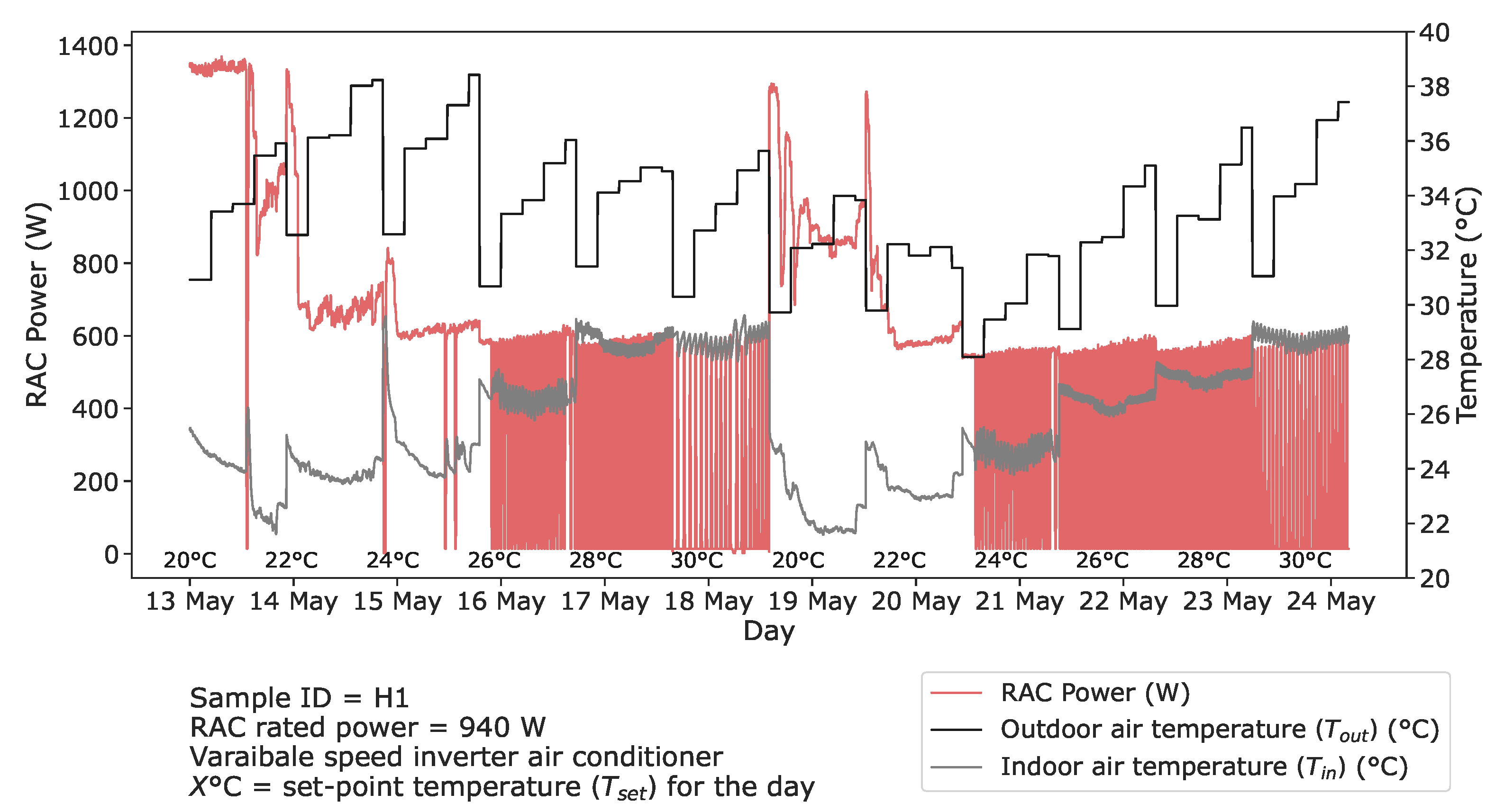
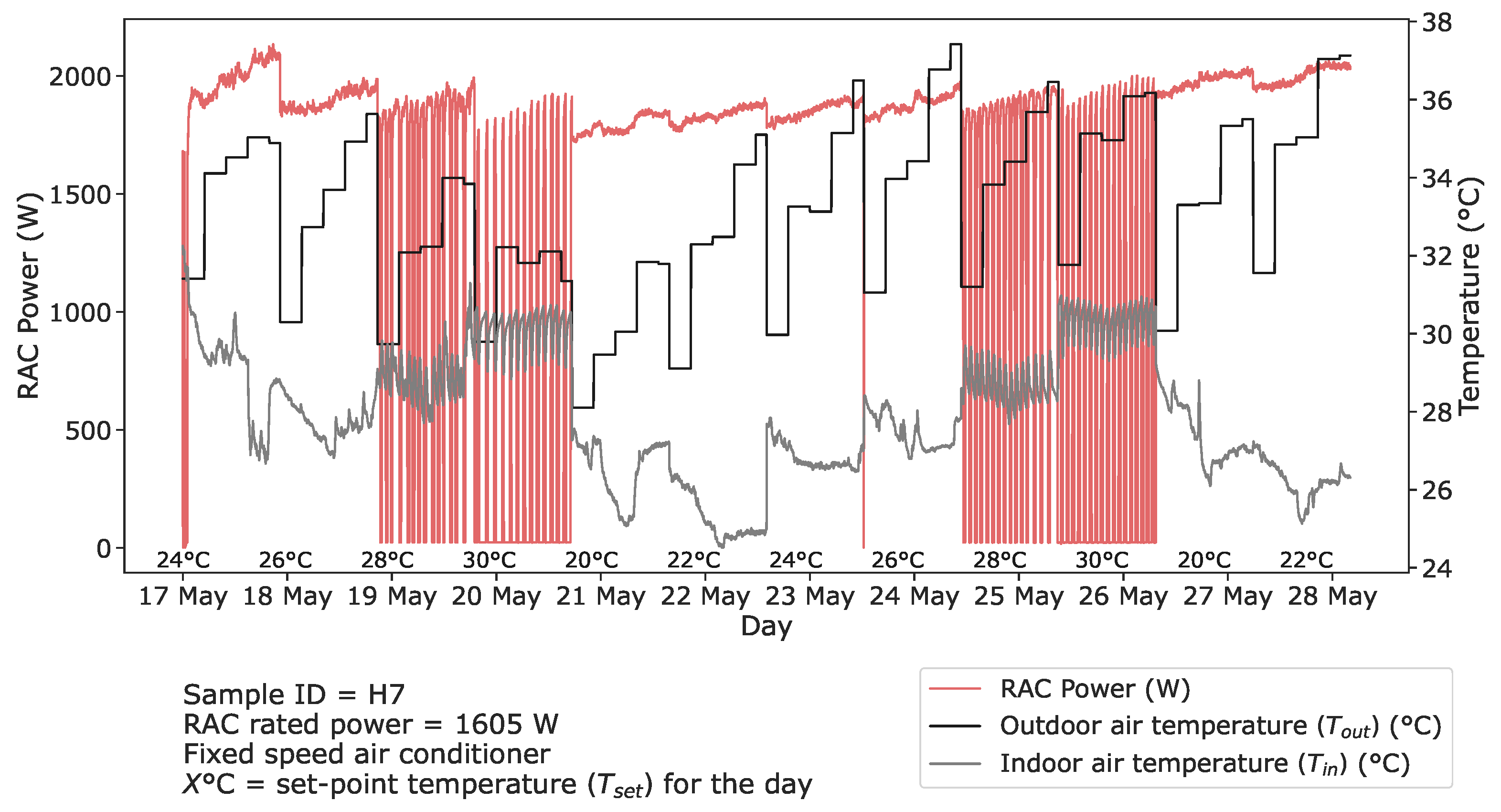
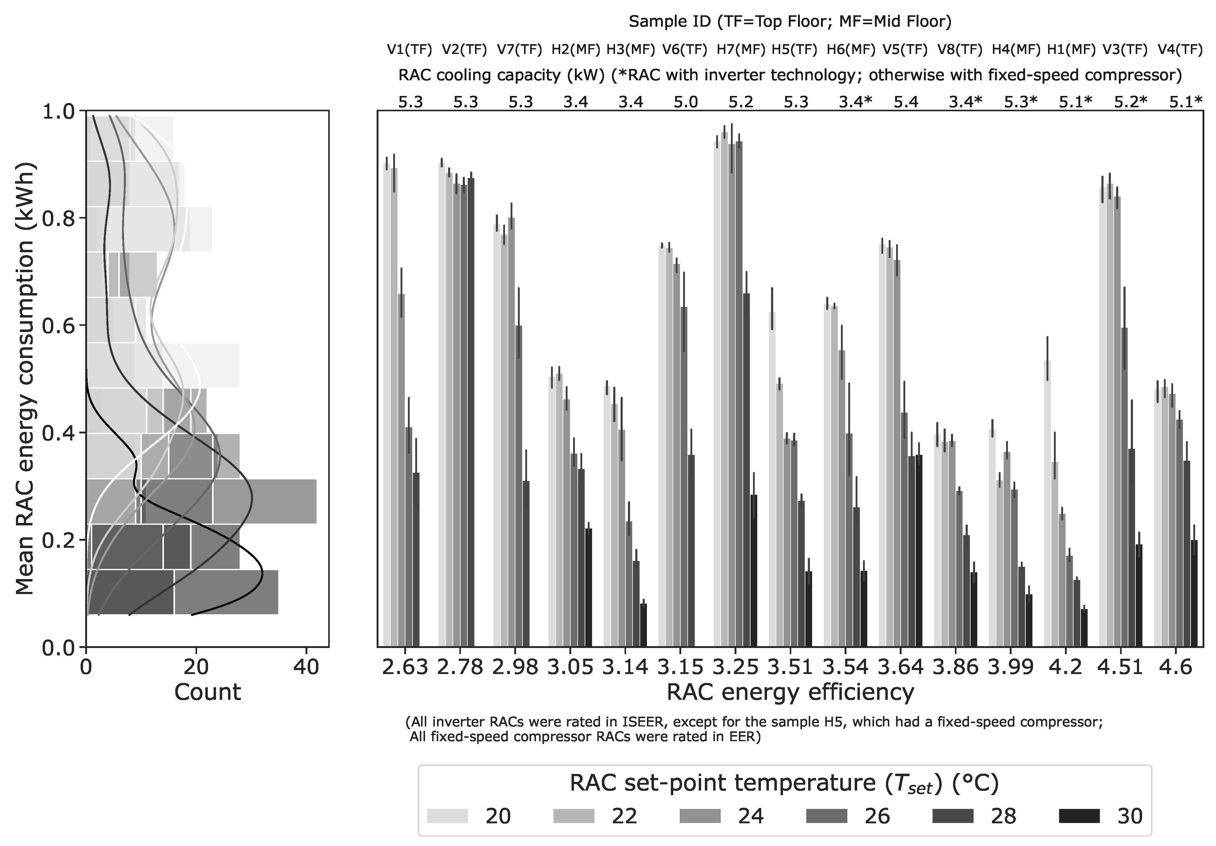
3.3. Energy Consumption

3.3.1. RAC Power Usage

Figure 8 shows the typical power consumption of an RAC with inverter technology at various set-point temperatures ( T s e t ). Outdoor air temperature ( T o u t ) and indoor air temperature ( T i n ) are also shown. At a T s e t of 20 ° C, the RAC operated continuously at more than 100% (full-load condition) of its rated power (940 W). At a T s e t of 22 ° C, it operated continuously at almost 60% (part-load condition) of its rated power. At all other set-point temperatures, it operated at close to 60% of its rated power and cycled frequently (i.e., the compressor would stop and start) depending on the load conditions.
Figure 9 shows the typical power usage of an RAC with a fixed-speed compressor. At all set-point temperatures, the RAC operated continuously above the rated power (1605 W), except at a T s e t of 28 and 30 ° C, where it cycled frequently.
The power consumption of all RACs at different set-point temperatures ( T s e t ) is shown in 15 bins in Figure 10. The colour gradient represents the amount of time (in minutes) in each bin. In general, at low set-point temperatures, e.g., at a T s e t of 20, 22 and 24 ° C, most RACs operated at 100% of their rated power or more in a few samples. Beyond a T s e t of 24 ° C, the RACs with inverter technology operated at part loads, reaching their minimum part loads at 28 and 30 ° C, where they cycled frequently, indicated by an increase in the amount of time near zero power. Most RACs with fixed-speed compressors operated at full load up to a T s e t of 26 ° C, at which point they started to cycle.

3.3.2. Ceiling Fan Power Usage

The current consumption of the step regulator and the USHA IR remote control increased approximately linearly and nonlinearly, respectively, with the fan speed settings (FSSs) (see Table 4). At high fan speed settings, there was a significant difference in power consumption between the step controller and the USHA IR remote control due to the differences between their regulator/dimmer circuits. Most fans had similar specifications and consumed little power compared with the RACs. Therefore, the fan power in all samples was calculated as follows: first, in the three samples V1, V4 and V5, the power consumption at different fan speed settings was obtained by multiplying the voltage and current consumption according to the USHA IR remote control; second, the average power consumption from these three samples was multiplied by a power factor of 0.8. This value was then used as the power consumption of the ceiling fan for all samples.

3.3.3. Total Energy Consumption

The energy consumption of the RAC was used for the analysis. The energy consumption per floor area was not considered because the cooling capacities and rated powers of all the RACs were different, as shown in Table 1. The bar plot of the total energy consumption of the RACs and ceiling fans over all days, samples and at different fan speed settings (FSSs) and set-point temperatures ( T s e t ) is shown in Figure 11A. The total energy consumption increased with the fan speed setting (FSS) and decreased with the set-point temperature ( T s e t ). Moreover, set-point temperature had a higher impact on the total energy consumption than the fan speed setting (see Figure 11B). However, the contribution of the ceiling fan to the total energy consumption increased at a T s e t of 28 and 30 ° C. To analyse the effect of the fan speed setting on the total energy consumption, the difference between the total energy consumption at different fan speed settings and at fan speed setting 1, given by E d i f f _ 1 , was analysed (see Figure 11C, D for the top and middle floors, respectively). This difference ( E d i f f _ 1 ) appeared to increase with the fan speed setting. This was particularly significant at high values of the set-point temperature (e.g., at a T s e t 28 and 30 ° C), at high fan speed settings and in samples with a roof (top floor). For better understanding of its significance, this energy difference, E d i f f _ 1 , is further discussed in relation to the corresponding temperature difference, T d i f f _ 1 , in Section 4.2.

3.3.4. Energy Saving due to Extended Set-Point Temperature

Energy savings in RACs at all fan speed settings (FSSs) resulting from set-point temperatures ( T s e t ) were compared against two baseline scenarios. The first scenario considered a T s e t of 20 ° C as the baseline (see Figure 12 (left)), and the second scenario considered the previous T s e t as the baseline (see Figure 12 (right)). Both scenarios are illustrated as bar plots with a 95% confidence interval. For both scenarios, energy savings are displayed, measured and adjusted for weather conditions. A polynomial relationship exists between energy savings and the set-point temperature ( T s e t ). In the scenario with a baseline T s e t of 20 ° C, the measured energy savings were statistically significant ( p ( β b 0 , β b 1 , β b 2 ) < 0.05 , R 2 = 0.752, adjusted R 2 = 0.746). In general, the measured energy savings were slightly higher than the weather-normalised energy savings. The weather normalised RAC energy consumption ( E n o r m ) was calculated as follows:
E n o r m = E m e a s C D D a c t _ s e t C D D 10 a v g _ s e t
where
  • E m e a s = measured RAC energy consumption (kWh);
  • C D D a c t _ s e t = cooling degree days with set-point temperature as base temperature during the study period (−);
  • C D D 10 a v g _ s e t = cooling degree days with set-point temperature as base temperature according to 10-year average weather data (−).
Figure 12. Effect of set-point temperature ( T s e t ) on RAC energy savings—A.
Energies 16 06807 g012
The average energy savings per 1 ° C increase in the set-point temperature ( T s e t ) were highly sensitive to the baseline. For example, compared with the baseline T s e t of 22 ° C, the means of the measured energy savings at a T s e t of 24, 26, 28 and 30 ° C were 7%, 26%, 48% and 69%, respectively (see Figure A9). Similarly, compared with a baseline T s e t of 24 ° C, the means of the measured energy savings at a T s e t of 26, 28 and 30 ° C were 21%, 44% and 67%, respectively.

3.3.5. Variation in RAC Energy Consumption due to Its Efficiency and Technology and Room Size and Construction

As the room size, construction and specifications of the RACs, i.e., their capacity, efficiency and technology, varied, Figure 13 (right) shows the bar plot (with 95% confidence intervals) of the RAC energy consumption in all samples at various set-point temperatures T s e t . The RAC efficiency in EER or ISEER is shown on the bottom horizontal axis. The sample ID, RAC cooling capacity and its type are shown on the upper horizontal axis. In general, the energy consumption decreased with an increase in the RAC efficiency, and a significant difference was observed above an efficiency of 3.64. Although the RAC in sample V3 was highly efficient with an ISEER of 4.51 and with inverter technology, the floor area was much higher compared with the other samples, and therefore, it had a high energy consumption. The energy consumption in samples with a RAC capacity of 1TR (V8, H2, H3 and H5) was lower than that of samples with a RAC capacity of 1.5 TR. Sample V8 was an exceptionally old leaky building with brickwork. Even with a low-capacity and high-efficiency RAC with inverter technology, its energy consumption was similar between a T s e t of 20 and 24 ° C. The histogram (see Figure 13 (left)) shows that in general, the energy consumption at a T s e t of 28 and 30 ° C was low across most samples.
Compressor technology had a significant impact on energy consumption. Depending on the set-point temperature ( T s e t ), RACs with inverter technology were found to consume approximately 34–68% less energy than RACs with fixed-speed compressors, as depicted in Figure 14 (left). The maximum difference between their energy consumption was 68% at a T s e t of 30 ° C, although the difference in absolute terms was small. The mean Power Factor of the RACs with inverter technology was lower compared with that of the fixed-speed RACs. Furthermore, the Power Factor in both categories declined with an increase in the set-point temperature ( T s e t ) (see Figure 14, right).

3.4. RAC User Behaviour

A total of 167 instances of switching the RACs on and off were accurately identified, with 82 instances of switch-on and 85 instances of switch-off recorded. These instances were correlated with the indoor conditions, indoor air temperature and relative humidity. The Shapiro–Wilk test, which assesses if a variable follows a normal distribution in a specific population, indicated that the instantaneous indoor air temperature ( T i n ) for the switch-on and switch-off of the RACs were normally distributed. However, this was not observed for the indoor relative humidity ( R H ). Furthermore, an independent T-test showed that the indoor air temperature ( t ( 19.4 ) , p < 0.0001 ) and relative humidity R H ( t ( 2.4 ) , p < 0.05 ) that switched the RACs on and off were significantly different and not random. The mean T i n at which the RACs were switched on and off was 31.9 ° C ( S D = 1.1 ) and 27.2 ° C ( S D = 1.8 ), respectively. The mean R H at which the RACs were switched on and off was 52.6% ( S D = 26.1 ) and 43.2% ( S D = 22.8 ), respectively. The difference between the mean T i n and R H at which the RACs were switched on and off, given by T o n _ o f f and R H o n _ o f f , was 4.7 ° C and 9.4%, respectively.
Figure 15 (right) shows the box plot of the instantaneous indoor air temperature ( T i n ) and relative humidity ( R H ) at which the RACs were switched on and off, and the thermal comfort bands according to the IMAC-R. In most cases, the RACs were switched on when the mean indoor air temperature was between the neutral operative temperature ( T n e u ) and upper 90% limit, with the exception of sample V7. The occupants in sample V7 seemed to tolerate a higher temperature than others before switching the RAC on and off. Most of the time, the RACs were switched off when the mean indoor air temperature was between the lower 90% and 80% limits. The occupants in Visakhapatnam (V2, V5 and V7), which has a warm and humid climate, appeared to tolerate higher relative humidity than the occupants in Hyderabad, which has a composite climate (H4 and H7), before turning on the RACs (see Figure 15 (left)). Except for sample H4, the mean relative humidity was always higher when the RACs were on than they were off.

4. Discussion

4.1. Limits for Tolerating Elevated Temperatures with Air Speed

In Indian Mixed-Mode Buildings (MMBs), ceiling fans are used first to mitigate thermal discomfort. Room Air-Conditioners (RACs) are used when ceiling fans alone, even at the highest fan speed settings, are not sufficient to maintain thermal comfort conditions. Studies in Indian buildings (mostly naturally-ventilated buildings) indicate that people are comfortable at temperatures up to 32 ° C, when there is a significant air velocity (see Section 1.4). In this study, the mean indoor air temperature ( T i n ) at which people switched on the RACs was 32 ° C, which is close to the values reported in the RAC user behaviour studies by [29,32]. This suggests that even when RACs are present, people tend to use the fans as much as they can. Beyond an indoor air temperature ( T i n ) of approximately 32 ° C, air velocity has an insufficient role in maintaining thermal comfort, as RACs are used to maintain thermal comfort. In addition, most people use ceiling fans and RACs simultaneously. Therefore, the use of ceiling fans can be considered as a baseline scenario for maintaining thermal comfort in Indian conditions, with or without the use of RACs.

4.2. Effect of Ceiling Fan Operation on Indoor Temperature and Energy Consumption

The effect of the indoor air velocity ( v e l ) from the ceiling fan on the indoor air temperature ( T i n ) and energy consumption was analysed through the difference between mean indoor air temperature at various fan speed settings and fan speed setting 1 ( T d i f f _ 1 ) and the difference between total energy consumption at various fan speed settings and fan speed setting 1 ( E d i f f _ 1 ), respectively. The temperature difference, T d i f f _ 1 , increased with the fan speed setting (see Figure 5). However, only limited information can be derived from the fan speeds 5D to 2D, as the indoor air temperature only seemed to stabilise at fan speed setting 1 in the test schedule used. From fan speed setting 2A, the temperature difference, T d i f f _ 1 , seemed to increase, especially in a few cases, e.g., at a T s e t of 20 ° C, in the top floors, and in most cases at fan speed setting 5A. An increase in fan speed setting (and consequently the indoor air velocity ( v e l ) may result in an increase in the indoor air temperature ( T i n ), e.g., due to an increase in the indoor heat transfer coefficient at high air speeds or to a lesser extent, the heat dissipated from fan motors. However, this increase may be mitigated by the RAC operation. Further insights can therefore be gained from the difference between total energy consumption at various fan speed settings and fan speed setting 1 ( E d i f f _ 1 ). The energy difference, E d i f f _ 1 , increased with the fan speed setting, particularly between fan speed setting 2A and 5A, and between the T s e t of 26 and 30 ° C (see Figure 11C,D). This may be because the RACs consume more energy to compensate for an increase in indoor air temperature. At low set-point temperatures, as the RACs were already operating at full-load conditions (see Figure 10), and therefore, the energy difference, E d i f f _ 1 , was insignificant, there was an increase in the temperature difference, T d i f f _ 1 . However, at high set-point temperatures, there was a significant decrease in the temperature difference, T d i f f _ 1 , and an increase in the energy difference, E d i f f _ 1 . In addition, the share of the ceiling fan energy consumption in the total energy consumption increased more strongly with the set-point temperature than with the fan speed setting. Overall, these results indicate that the energy consumption of the RAC, and consequently the total energy consumption, increased with the fan speed setting.

4.3. RAC Energy Savings due to Air Speed

We analysed the two questions discussed in Section 1.3.
  • First, did the use of the fan lead to a reduction in the duration of RAC use?
  • Second, whether the use of fans or an increase in fan speed setting resulted in extending the set-point temperature ( T s e t )?
Considering a baseline scenario that the ceiling fans are always used with or without RACs (see Section 4.1), a priori energy savings that might have been expected due to fan use or increased fan speed setting are purely notional and may not exist in practice. Studies have shown that users typically operate RACs at a T s e t of 24–26 ° C. However, in this study, at a T s e t of 28–30 ° C, the mean indoor air temperature was mostly between neutral operative temperature and the lower 90% limit (except at fan speed setting 5A). This indicates that at these values of set-point temperature, comfort conditions can be maintained regardless of the fan speed setting. If some air movement is desired even when the RACs are in use, less energy is required at fan speed setting 1 (see Section 4.2). It can be concluded that in the context of India, increasing the fan speed setting while using RACs will not lead to any energy savings. On the contrary, it will result in excess energy consumption.

4.4. RAC Energy Savings due to Set-Point Temperature and Operation

As the set-point temperature increased from 20 to 24 ° C, the study shows that the weather normalised RAC energy consumption ( E n o r m ) was 14% and the average energy savings per 1 ° C increase in T s e t were 3.5% (compared with the BEE’s estimate of 6%). In addition, at lower set-point temperatures, energy was consumed to meet the latent load (see Figure 6), i.e., to dehumidify the space. However, the adaptive comfort model IMAC-R is independent of the relative humidity. Moreover, relative humidity did not appear to have a significant effect on the RAC switch on and off behaviour in comparison with the indoor air temperature ( T i n ). However, as the set-point temperature increased from a baseline T s e t of 24 ° C to 26 ° C, and from a baseline T s e t of 26 ° C to 28 ° C, the mean weather normalised RAC energy consumption was 10% and 26%, respectively. This means that the average energy savings per 1 ° C increase in set-point temperature ( T s e t ) were 5% and 13%, respectively. Compared with the T s e t of 20, 22, 24, 26 and 28 ° C as baseline and the T s e t of 30 ° C as target, the average energy savings per 1 ° C increase in T s e t were 7, 9, 11 and 14 and 20%, respectively. In general, the energy savings in the study were sensitive to, and increased with, the baseline and difference between the baseline and target values of the set-point temperature T s e t (see Figure 12 and Figure A9). Furthermore, there is a high degree of variation in the data when the RACs were switched off (see Section 3.4), which indicated that RACs were not switched off efficiently. That is, there is a tendency for people to ignore the need to increase the set-point temperature or switch off the RACs until they feel cold. Therefore, there is considerable potential to minimise energy consumption by optimising the RAC’s on and off control or set-point temperature ( T s e t ) control based on the measured indoor air temperature ( T i n ).

4.5. Strengths and Limitations of the Methodology

The choice of location, time and duration was based on the balance of opportunities and constraints for conducting the field study. The opportunities are listed below.
  • Bedrooms in residential buildings are unoccupied during the day making it convenient to test different set-point temperatures and fan speed settings.
  • The results of the study reflect the actual usage times of the RACs in residential buildings (see Section 1.4)
  • A range of housing typologies were covered, e.g., single-family houses (one-, two- and three-storey buildings) and multifamily houses (e.g., apartments with up to seven storeys).
  • The study results are also applicable to small offices, as most share similar characteristics of space size, construction, RAC type and cooling capacity.
Despite the limitations listed below, we believe that the results still provide useful insights and meet the study objectives.
  • Where there was a significant effect on the results due to building (age, orientation and surroundings) or RAC specifications, this was discussed in the results (see Section 3.3.5).
  • The sample size for RAC energy consumption (15), indoor conditions (12) and RAC user behaviour analysis (6) was limited. However, weather-normalised energy savings were presented for the study period. The study period was limited to 24 days and did not cover the entire cooling season. However, it coincided with extreme outdoor weather conditions in one city and near extreme weather conditions in the other city. In addition, apart from survey-based studies, there are few field studies that have exclusively monitored RAC energy consumption and indoor conditions in India. One field study of RAC use in India used a sample size of eight dwellings and analysed data for 30 days [29].
  • This is not a thermal comfort study and therefore, an exclusive user survey on thermal comfort or RAC usage behaviour was not conducted.

5. Conclusions

In this study, the energy consumption of Room Air-Conditioners (RACs) and ceiling fans at different set-point temperature ( T s e t ) and fan speed settings (FSSs) was analysed in relation to the indoor conditions and the Indian Model for Adaptive Comfort-Residential (IMAC-R). In addition, RAC usage behaviour and the energy performance of RACs with inverter technology and fixed-speed compressors were analysed. The results showed that average energy savings due to a change in the set-point temperature ( T s e t ) were highly sensitive to the baseline set-point temperature. An often-made assumption that a “1 ° C increase in the set-point temperature ( T s e t ) results in 6% average energy savings” can be misleading, as the energy savings between the set-point temperatures is polynomial and not linear. Policymakers will also find these results useful for MEPS policy, default set-point temperature recommendations and energy conservation. Increasing the fan speed setting during the RAC operation leads to unnecessary energy consumption without any significant enhancement to thermal comfort conditions. This finding contrasts with the results reported in the literature, which often do not take into account air movement or the use of fans in the baseline case. Therefore, space-cooling energy savings due to air speed should be estimated by using appropriate assumptions for actual fan usage behaviour as a baseline scenario. Significant energy savings could be achieved by optimising RAC control, such as on/off control or changing the set-point temperature ( T s e t ), using Internet of Things (IoT) devices and machine learning methods. Further research is needed to investigate the relationship between the set-point temperature ( T s e t ) and thermal comfort and to optimise RAC operation. In this study, we presented novel and cost-effective IoT instruments that could be used for such further research. The use of fans for air movement is a prevalent practice in many tropical regions worldwide. With the rising use of air-conditioning units in such areas, the study’s outcomes offer significant potential for reducing energy consumption in space cooling and the resultant greenhouse gas (GHG) emissions.

Author Contributions

Conceptualization, S.G., C.v.T. and R.R.; methodology, S.G., C.v.T. and R.R.; formal analysis, S.G.; investigation, S.G.; data curation, S.G.; writing—original draft preparation, S.G.; writing—review and editing, C.v.T., R.R. and S.T.; visualization, S.G.; supervision, C.v.T., R.R. and S.T.; funding acquisition, S.G. and S.T. All authors have read and agreed to the published version of the manuscript.

Funding

We have received with thanks a grant for purchase of the instruments used in this study from The Friends of the Wuppertal Institute (Die Vereinigung der Freunde des Wuppertal Instituts), Germany, a nonprofit association. We acknowledge financial support by Wuppertal Institut für Klima, Umwelt, Energie gGmbH within the funding programme Open Access Publishing.

Informed Consent Statement

The authors declare that they have received informed consent from the human participants. A formal approval from the ethics committee was not required because the study only consisted of nonintrusive passive observations. It did not involve any interaction with the participants.

Data Availability Statement

The data contain sensitive information and therefore cannot be made available.

Acknowledgments

We are grateful to all the volunteers who participated in the study. We thank the anonymous reviewers for their feedback. Their comments improved the readability of the manuscript.

Conflicts of Interest

The authors declare no conflict of interest.

Acronyms

ABSAcrylonitrile Butadiene Styrene
BEEBureau of Energy Efficiency
EEREnergy Efficiency Ratio
EPWEnergy Plus Weather Format
FSSfan speed setting
GHGgreenhouse gas
HTTPHypertext Transfer Protocol
IMACIndian Model for Adaptive Comfort
IMAC-RIndian Model for Adaptive Comfort-Residential
IoTInternet of Things
IRInfrared
ISEERIndian Seasonal Energy Efficiency Ratio
JSTJapan Solderless Terminal
MEPSMinimum Efficiency Performance Standards
MMBMixed-Mode Building
NBCNational Building Code
NVnaturally-ventilated
PFPower Factor
PHPHypertext Preprocessor
RACRoom Air-Conditioner
RCCReinforced Cement Concrete
RPMrotations per minute
RTCReal Time Clock
S&LStandards and Labelling
TMYTypical Meteorological Year
TSITropical Summer Index
UPVCUnplasticised Polyvinyl Chloride
USNBSUnited States National Bureau of Standards
WWRWindow-to-Wall (area) Ratio

Nomenclature

SymbolDescriptionUnit
C D D 10 a v g _ s e t cooling degree days with set-point temperature as base temperature according to 10-year average weather data-
C D D a c t _ s e t cooling degree days with set-point temperature as base temperature during the study period-
C M M cubic meter per minute m 3 / min
E d i f f _ 1 difference between total energy consumption at various fan speed settings and fan speed setting 1 kWh
E m e a s measured RAC energy consumption kWh
E n o r m weather normalised RAC energy consumption kWh
Ffrequency Hz
Icurrent Amp
P F power factor-
Ppower W
R H o n _ o f f difference between instantaneous mean relative humidity when the RACs were turned on and off%
R H relative humidity%
T d i f f _ 1 difference between mean indoor air temperature at various fan speed settings and fan speed setting 1 ° C
T g globe temperature ° C
T i n indoor air temperature ° C
T m r t mean radiant temperature ° C
T n e u neutral operative temperature ° C
T o n _ o f f difference between instantaneous mean air temperature when the RACs were turned on and off ° C
T o p indoor operative temperature ° C
T o u t outdoor air temperature ° C
T s e t set-point temperature ° C
Vvoltage V
h i internal surface heat transfer coefficient m 2 K / W
v e l indoor air velocity m / s
U-valuethermal transmittance W / m 2 K

Appendix A. Instrumentation

Appendix A.1. Instrument Sensors and Components

Table A1 shows the details of various components and sensors used in the custom-built comfort, energy and IR modules (including their libraries) and other instruments used in the study.
Table A1. Instrument sensors and components.
ModuleMake of the Sensor or ComponentLibraryMeasurement/DescriptionUnitAccuracy
Comfort moduleWemos SHT30 (Sensirion SHT30 sensor)[36]Indoor air temperature ( T i n ) ° C±3
Relative humidity ( R H )%±0.3
Maxim Integrated DS18B20[52]Globe temperature ( T g ) ° C±0.5
Generic SD card + RTC module[53,54]SD card for data logging and RTC to record the timestamp
Energy modulePZEM–004T 3.0 TTL Modbus–RTU by peacefair[55]Voltage (V)V±0.5%
Current (I)Amp±0.5%
Power (P)W±0.5%
Power factor (PF)-±0.5%
Frequency (F)Hz±0.5%
Generic SD card + RTC module[53,54]SD card for data logging and RTC to record the timestamp
IR emitter moduleGrove–Infrared Emitter (VISHAY TSAL6200 IR LED)[56]IR emitter LED
Generic RTC module[53]RTC module to keep time
Ceiling fan remote controlUSHA IR remote controller Speed controller for ceiling fan
Hot wire anemometerTrotec TA 300 Indoor air velocity ( v e l )m/s±5%
Clamp on multimeterKAIWEETS HT206B Current Clamp Meter Voltage (V)V±(1%+3)
Current (I)Amp±(2.5%+5)

Appendix A.2. Custom-Built Modules Used in the Study

In general, all modules used in the study were built in a modular way and enclosed in Acrylonitrile Butadiene Styrene (ABS) plastic boxes. The following steps describe the building of the IoT modules used in the study.

Appendix A.2.1. Base Data-Logger Unit

A microcontroller base data-logger unit was first assembled. For comfort, energy and IR emitter modules, this consisted of a WEMOS D1 mini pro [57] microcontroller board (with pin headers) and a micro-SD card + RTC shield (with pin headers) (see Figure A1a,b) put in place on a triple base (for comfort and energy modules). The WEMOS D1 mini pro and micro–SD card + RTC shield were soldered with female header pins towards the bottom side, which locked themselves into the female pin headers on the top side of the triple base. Similarly, for the IR receiver module, a WEMOS D1 mini [58] microcontroller board (with pin headers) was used with a micro-SD card + RTC shield put in place on a WEMOS D1 mini dual base (see Figure A1c). The RTC used an I 2 C interface (pins D1 and D2) and the micro-SD card shield used four pins (D5, D6, D7, D8) on the microcontroller board. Additionally, appropriate female Japan Solderless Terminal (JST) pins were soldered to corresponding pins on the microcontroller board and glued to the base unit. The WEMOS D1 mini pro comes with an on-board female JST pin. The pin headers and JST connections provide the units with flexible yet secure connections. They make the units modular, and it is easy to change individual components when they malfunction.
Figure A1. Base units. (a) Microcontroller base data-logger unit. (b) Base data–logger unit assembled. (c) IR emitter data-logger base unit.
Energies 16 06807 g0a1

Appendix A.2.2. Comfort Module

A WEMOS SHT30 shield was used for measuring T i n and R H . The WEMOS SHT30 shield uses an I 2 C interface to communicate with the WEMOS D1 mini microcontroller board. It comes with an on-board female JST pin (see Figure A2a). A JST connector was used to connect the female JST pins on the WEMOS SHT30 shield and base data-logger unit.
Figure A2. Comfort module build-up. (a) SHT30 T i n and R H sensor with JST connector. (b) DS18B20 sensor fitted inside a ping-pong ball. (c) DS18B20 sensor with JST connector. (d) Plastic mount for sensors. (e) Comfort module showing the JST connections. (f) Comfort module enclosed.
Energies 16 06807 g0a2
A Maxim Integrated DS18B20 one-wire digital temperature sensor air-tightly sealed in a black matt painted ping-pong ball was used to measure T g and subsequently calculate T m r t by using T g (see Figure A2b). DS18B20 uses a ground pin, 5 V pin and a digital pin on the WEMOS D1 mini microcontroller board. The three pins of the DS18B20 were soldered to a JST connector (see Figure A2c), which was inserted into the female JST pin on the base data-logger unit. In addition, a 4.7K ohm pull-up resistor was placed between the data (digital pin) and the 5 V pin (soldered on the base data-logger unit) (see Figure A1).
A black pipe of 12 mm diameter and 15 cm length was used to mount the ping-pong ball with the DS18B20 sensor and the WEMOS SHT30 over the comfort unit enclosure (see Figure A2d). An IP68 waterproof cable gland was used to mount the pipe. In addition, the pipe was perforated to ensure air movement and avoid the influence of heat from the data-logger unit on both the sensors due to stack effect. The base unit was then enclosed in an ABS plastic box (see Figure A2e,f).

Appendix A.2.3. IR Modules

A Grove-IR emitter, which uses a VISHAY TSAL6200 IR LED, was used in the IR controller unit and to transmit infrared signals (see Figure A3a). The IR emitter uses a ground pin, 5 V pin and a digital pin on the WEMOS D1 mini microcontroller board. Its emitter comes with an on-board female JST pin, which was then connected to the base data-logger unit using a suitable JST connector (see Figure A3c) and enclosed in an ABS plastic box (see Figure A3b).
Figure A3. IR modules build-up. (a) Grove IR emitter module. (b) IR emitter module. (c) IR emitter module showing JST connection.
Energies 16 06807 g0a3

Appendix A.2.4. Energy Module

A PZEM-004T 3.0 TTL Modbus-RTU module by peacefair was used to measure the RAC energy consumption. It uses ground, 5 V, Tx and Rx pins on the microcontroller. The PZEM-004T comes with an on-board female JST pin, which was then connected to the base data-logger unit using a suitable JST connector (see Figure A4a). The entire assembly was then encased in an IP54-rated plastic box (see Figure A4b).
Figure A4. Comfort module build-up. (a) Components of the energy module. (b) Energy module casing.
Energies 16 06807 g0a4

Appendix A.3. IoT Communication

The IoT communication between the modules and a remote MySQL database was made by using an HTTP POST request to a PHP script to insert data (sensor readings) into a MySQL database by using the code and method described by [46]. For this purpose, a web domain and space on a commercial web hosting platform were set up. The data from the modules were sent as an HTTP POST request to the domain via Wi-Fi. Whenever a POST was sent, a PHP script on the hosting platform recorded the data in the MySQL database.

Appendix B. Representative Pictures of the Samples

Figure A5. Sample V1. (a) Exterior view of sample house V1. (b) Interior view of the experimental room in sample house V1.
Energies 16 06807 g0a5
Figure A6. Sample V3. (a) Exterior view of sample house V3. (b) Interior view of the experimental room in sample house V3.
Energies 16 06807 g0a6
Figure A7. Exterior views of some samples. (a) Exterior view of sample house V4. (b) Exterior view of sample house V6.
Energies 16 06807 g0a7
Figure A8. Interior views of some samples. (a) Interior view of sample house V2. (b) Interior view of sample house H2.
Energies 16 06807 g0a8

Supplementary Figures

Figure A9. Effect of set-point temperature ( T s e t ) on RAC energy savings—B.
Energies 16 06807 g0a9

References

  1. IEA. Cooling. Available online: https://www.iea.org/energy-system/buildings/space-cooling (accessed on 28 August 2023).
  2. Indraganti, M. Thermal adaption and impediments: Findings from a field study in Hyderabad, India. In Proceedings of the Adapting to Change: New Thinking on Comfort Cumberland Lodge, Windsor, UK, 9–11 April 2010. [Google Scholar]
  3. Honnekeri, A.; Brager, G.; Dhaka, S.; Mathur, J. Comfort and adaptation in mixed-mode buildings in a hot-dry climate. In Proceedings of the 8th Windsor Conference, Windsor, UK, 10–13 April 2014. [Google Scholar]
  4. Indraganti, M.; Ooka, R.; Rijal, H.B.; Brager, G.S. Drivers and barriers to occupant adaptation in offices in India. Archit. Sci. Rev. 2015, 58, 77–86. [Google Scholar] [CrossRef]
  5. Yawale, S.K.; Hanaoka, T.; Kapshe, M. Development of energy balance table for rural and urban households and evaluation of energy consumption in Indian states. Renew. Sustain. Energy Rev. 2021, 136, 110392. [Google Scholar] [CrossRef]
  6. BEE. Bureau of Energy Efficiency (Particulars and Manner of their Display on Labels of Room Air Conditioners) Regulations. 2017. Available online: https://beestarlabel.com/Content/Files/IAC_Notification.pdf (accessed on 15 October 2022).
  7. Rawal, R.; Shukla, Y.; Vardhan, V.; Asrani, S.; Schweiker, M.; de Dear, R.; Garg, V.; Mathur, J.; Prakash, S.; Diddi, S.; et al. Adaptive thermal comfort model based on field studies in five climate zones across India. Build. Environ. 2022, 219, 109187. [Google Scholar] [CrossRef]
  8. ANSI/ASHRAE 55-2020; Thermal Environmental Conditions for Human Occupancy. American National Standards Institute ASHRAE: Washington, DC, USA, 2020.
  9. Givoni, B. Man, Climate and Architecture; Elsevier: Amsterdam, The Netherlands, 1969. [Google Scholar]
  10. Epstein, Y.; Moran, D.S. Thermal comfort and the heat stress indices. Ind. Health 2006, 44, 388–398. [Google Scholar] [CrossRef]
  11. Luo, M.; Zhang, H.; Wang, Z.; Arens, E.; Chen, W.; Bauman, F.S.; Raftery, P. Ceiling-fan-integrated air-conditioning: Thermal comfort evaluations. Build. Cities 2021, 2, 928–951. [Google Scholar] [CrossRef]
  12. Rohles, F.H.; Konz, S.A.; Jones, B.W. Enhancing Thermal Comfort with Ceiling Fans. In Proceedings of the Human Factors Society Annual Meeting; SAGE Publications: Los Angeles, CA, USA, 1982. [Google Scholar] [CrossRef]
  13. Zhai, Y.; Zhang, Y.; Zhang, H.; Pasut, W.; Arens, E.; Meng, Q. Human comfort and perceived air quality in warm and humid environments with ceiling fans. Build. Environ. 2015, 90, 178–185. [Google Scholar] [CrossRef]
  14. He, Y.; Chen, W.; Wang, Z.; Zhang, H. Review of fan-use rates in field studies and their effects on thermal comfort, energy conservation, and human productivity. Energy Build. 2019, 194, 140–162. [Google Scholar] [CrossRef]
  15. Sharma, M.R.; Ali, S. Tropical summer index—A study of thermal comfort of Indian subjects. Build. Environ. 1986, 21, 11–24. [Google Scholar] [CrossRef]
  16. Manu, S.; Shukla, Y.; Rawal, R.; Thomas, L.E.; Dear, R.; Dave, M.; Vakharia, M. Assessment of Air Velocity Preferences and Satisfaction for Naturally Ventilated Office Buildings in India. In Proceedings of the Passive and Low Energy Architecture (PLEA) Annual International Conference, Ahmedabad, India, 16–18 December 2014. p. 8.
  17. Kumar, S.; Mathur, J.; Mathur, S.; Singh, M.K.; Loftness, V. An adaptive approach to define thermal comfort zones on psychrometric chart for naturally ventilated buildings in composite climate of India. Build. Environ. 2016, 109, 135–153. [Google Scholar] [CrossRef]
  18. Sansaniwal, S.K.; Tewari, P.; Kumar, S.; Mathur, S.; Mathur, a.J. Impact assessment of air velocity on thermal comfort in composite climate of India. Sci. Technol. Built Environ. 2020, 26, 1301–1320. [Google Scholar] [CrossRef]
  19. BIS. National Building Code; Bureau of Indian Standards: New Delhi, India, 2016; Volume 2.
  20. Malik, A.; Bongers, C.; McBain, B.; Rey-Lescure, O.; Dear, R.d.; Capon, A.; Lenzen, M.; Jay, O. The potential for indoor fans to change air conditioning use while maintaining human thermal comfort during hot weather: An analysis of energy demand and associated greenhouse gas emissions. Lancet Planet. Health 2022, 6, e301–e309. [Google Scholar] [CrossRef] [PubMed]
  21. Amoabeng, K.O.; Opoku, R.; Boahen, S.; Obeng, G.Y. Analysis of indoor set-point temperature of split-type ACs on thermal comfort and energy savings for office buildings in hot-humid climates. Energy Built Environ. 2023, 4, 368–376. [Google Scholar] [CrossRef]
  22. Angelopoulos, C.; Cook, M.J.; Spentzou, E.; Shukla, Y. Energy Saving Potential of Different Setpoint Control Algorithms in Mixed-Mode Buildings. In Proceedings of the BSO 2018, Cambridge, UK, 11–12 September 2018; p. 8. [Google Scholar]
  23. Bienvenido-Huertas, D.; Sánchez-García, D.; Pérez-Fargallo, A.; Rubio-Bellido, C. Optimization of energy saving with adaptive setpoint temperatures by calculating the prevailing mean outdoor air temperature. Build. Environ. 2020, 170, 106612. [Google Scholar] [CrossRef]
  24. Lamsal, P.; Bajracharya, S.B.; Rijal, H.B. A Review on Adaptive Thermal Comfort of Office Building for Energy-Saving Building Design. Energies 2023, 16, 1524. [Google Scholar] [CrossRef]
  25. DSM Cell, Tata Power, Mumbai. Demand Side Management. In Proceedings of the 14th Annual General Body Meeting of FOIR. Available online: https://www.tatapower.com/investor-relations/tata-power-2022/pdf/boards-Report.pdf (accessed on 10 August 2023).
  26. Prayas (Energy Group). Residential Electricity Consumption in India: What Do We Know? Available online: https://energy.prayaspune.org/our-work/research-report/residential-electricity-consumption-in-india-what-do-we-know#:~:text=The%20residential%20electricity%20consumption%20(REC,household%20incomes%2C%20and%20technology%20development (accessed on 30 August 2022).
  27. Electric Utility Load Research and DSM Programme Design Utility CEO Forum on Demand Side Management. Available online: https://shaktifoundation.in/wp-content/uploads/2017/06/background-paper_third-meeting_final.pdf (accessed on 29 August 2022).
  28. Khosla, R.; Agarwal, A.; Sircar, N.; Chatterjee, D. The what, why, and how of changing cooling energy consumption in India’s urban households. Environ. Res. Lett. 2021, 16, 044035. [Google Scholar] [CrossRef]
  29. Gupta, R.; Antony, A.; Garg, V.; Mathur, J. Investigating the relationship between residential AC, indoor temperature and relative humidity in Indian dwellings. J. Physics Conf. Ser. 2021, 2069, 012103. [Google Scholar] [CrossRef]
  30. Indraganti, M.; Ooka, R.; Rijal, H.B. Thermal comfort in offices in India: Behavioral adaptation and the effect of age and gender. Energy Build. 2015, 103, 284–295. [Google Scholar] [CrossRef]
  31. Peeters, L.; Beausoleil-Morrison, I.; Novoselac, A. Internal convective heat transfer modeling: Critical review and discussion of experimentally derived correlations. Energy Build. 2011, 43, 2227–2239. [Google Scholar] [CrossRef]
  32. Gokarakonda, S.; van Treeck, C.; Rawal, R. Investigating Optimum Cooling Set Point Temperature and Air Velocity for Thermal Comfort and Energy Conservation in Mixed-Mode Buildings in India. Energies 2022, 15, 2259. [Google Scholar] [CrossRef]
  33. PIB. Frequently Asked Questions on BEE Recommendations on Temperature Setting of Air Conditioners; Press Information Bureau: New Delhi, India, 2018. Available online: https://pib.gov.in/newsite/PrintRelease.aspx?relid=180281 (accessed on 29 July 2022).
  34. Projecting National Energy Saving Estimate from the Adoption of Adoption of Adaptive Thermal Comfort Standards in 2030. Available online: http://www.aeee.in/wp-content/uploads/2018/09/Adoption-of-Adaptive-Thermal-Comfort-Standards-in-2030.pdf (accessed on 11 November 2018).
  35. James, P.W.; Sonne, J.K.; Vieira, R.K.; Parker, D.S.; Anello, M.T. Are Energy Savings Due to Ceiling Fans Just Hot Air? In 1996 Summer Study Conference ‘Profiting from Energy Efficiency’; ACEEEE Summer Study on Energy Efficiency in Buildings; Pacific Grove, CA, USA. 1996, p. 7. Available online: https://www.aceee.org/files/proceedings/1996/data/papers/SS96_Panel8_Paper10.pdf (accessed on 10 August 2023).
  36. Arduino Library for the WEMOS SHT30 Shiled. Available online: https://github.com/wemos/WEMOS_SHT3x_Arduino_Library (accessed on 15 December 2021).
  37. Chen, W.; Zhang, H.; Arens, E.; Luo, M.; Wang, Z.; Jin, L.; Liu, J.; Bauman, F.S.; Raftery, P. Ceiling-fan-integrated air conditioning: Airflow and temperature characteristics of a sidewall-supply jet interacting with a ceiling fan. Build. Environ. 2020, 171, 106660. [Google Scholar] [CrossRef]
  38. Suryono, W.; Prabowo, A.S.; Suhanto; Sazali, A.M. Monitoring and controlling electricity consumption using Wemos D1 Mini and smartphone. IOP Conf. Ser. Mater. Sci. Eng. 2020, 909, 012014. [Google Scholar] [CrossRef]
  39. de Dear, R. Ping-pong globe thermometers for mean radiant temperatures. H V Eng. 1988, 60, 10–11. [Google Scholar]
  40. Humphreys, M.A. The optimum diameter for a globe thermometer for use indoors. Ann. Occup. Hyg. 1977, 20, 135–140. [Google Scholar] [CrossRef] [PubMed]
  41. ISO 7726:1998; Ergonomics of the Thermal Environment—Instruments for Measuring Physical Quantities. ISO: Geneva, Switzerland, 1998.
  42. d’Ambrosio Alfano, F.R.; Ficco, G.; Frattolillo, A.; Palella, B.I.; Riccio, G. Mean Radiant Temperature Measurements through Small Black Globes under Forced Convection Conditions. Atmosphere 2021, 12, 621. [Google Scholar] [CrossRef]
  43. Teitelbaum, E.; Alsaad, H.; Aviv, D.; Kim, A.; Voelker, C.; Meggers, F.; Pantelic, J. Addressing a systematic error correcting for free and mixed convection when measuring mean radiant temperature with globe thermometers. Sci. Rep. 2022, 12, 6473. [Google Scholar] [CrossRef]
  44. Jain, A.; Upadhyay, R.R.; Chandra, S.; Saini, M.; Kale, S. Experimental Investigation of the Flow Field of a Ceiling Fan. In Proceedings of the Heat Transfer Summer Conference, Charlotte, NC, USA, 11–15 July 2004; pp. 93–99. [Google Scholar] [CrossRef]
  45. MySQL. Available online: https://www.mysql.com/ (accessed on 15 March 2022).
  46. ESP32/ESP8266 Insert Data into MySQL Database|Random Nerd Tutorials. Available online: https://randomnerdtutorials.com/esp32-esp8266-mysql-database-php/ (accessed on 2 December 2022).
  47. Pandas-Dev/Pandas: Pandas 1.0.3. Available online: https://zenodo.org/record/3715232 (accessed on 15 March 2022).
  48. Virtanen, P.; Gommers, R.; Oliphant, T.E.; Haberland, M.; Reddy, T.; Cournapeau, D.; Burovski, E.; Peterson, P.; Weckesser, W.; Bright, J.; et al. SciPy 1.0: Fundamental Algorithms for Scientific Computing in Python. Nat. Methods 2020, 17, 261–272. [Google Scholar] [CrossRef]
  49. Seabold, S.; Perktold, J. Statsmodels: Econometric and statistical modeling with python. In Proceedings of the 9th Python in Science Conference, Austin, TX, USA, 28 June–3 July 2010. [Google Scholar]
  50. Hunter, J.D. Matplotlib: A 2D graphics environment. Comput. Sci. Eng. 2007, 9, 90–95. [Google Scholar] [CrossRef]
  51. Mwaskom/Seaborn: v0.8.1 (September 2017). Available online: https://zenodo.org/record/883859 (accessed on 10 August 2023).
  52. DS18B20. Available online: https://github.com/matmunk/DS18B20 (accessed on 15 December 2021).
  53. Adafruit Industries. RTClib. Available online: https://github.com/adafruit/RTClib (accessed on 15 December 2021).
  54. Arduino Libraries. SD Library for Arduino. Available online: https://github.com/arduino-libraries/SD (accessed on 15 December 2021).
  55. PZEM-004T v3.0. Available online: https://github.com/mandulaj/PZEM-004T-v30 (accessed on 28 February 2022).
  56. Crankyoldgit/IRremoteESP8266. Available online: https://github.com/crankyoldgit/IRremoteESP8266 (accessed on 15 December 2021).
  57. D1 Mini Pro—WEMOS Documentation. Available online: https://www.wemos.cc/en/latest/d1/d1_mini_pro.html (accessed on 2 December 2022).
  58. LOLIN D1 Mini—WEMOS Documentation. Available online: https://www.wemos.cc/en/latest/d1/d1_mini.html (accessed on 2 December 2022).
Figure 1. Representative image of a typical room.
Energies 16 06807 g001
Figure 2. Outdoor weather in Visakhapatnam. Grey area indicates duration of study.
Energies 16 06807 g002
Figure 3. Outdoor weather in Hyderabad. Grey area indicates duration of study.
Energies 16 06807 g003
Figure 4. Indoor air temperature across the samples during the study.
Energies 16 06807 g004
Figure 5. Difference between mean indoor air temperature at various fan speed settings and fan speed 1.
Energies 16 06807 g005
Figure 6. Indoor relative humidity across samples during the study.
Energies 16 06807 g006
Figure 7. Air velocity in the jet core directly below the ceiling fan on top and middle floors (m/s).
Energies 16 06807 g007
Figure 8. Power consumption of RAC with inverter technology.
Energies 16 06807 g008
Figure 9. Power consumption of an RAC with a fixed-speed compressor.
Energies 16 06807 g009
Figure 10. Power consumption of the RACs at various values of set-point temperature ( T s e t ).
Energies 16 06807 g010
Figure 11. Effect of ceiling fan speed on energy consumption.(A) Total energy consumption at various fan speed settings; (B) Fraction of ceiling fan in total energy consumption at various fan speed settings; (C) Difference between total energy consumption at various fan speed settings and fan speed setting in the top floors (D) Difference between total energy consumption at various fan speed settings and fan speed setting in the middle floors.
Energies 16 06807 g011
Figure 13. Effect of the RAC energy efficiency on energy consumption. *RAC with inverter technology; otherwise with fixed-speed compressor.
Energies 16 06807 g013
Figure 14. Effect of inverter technology on RAC energy consumption and power factor.
Energies 16 06807 g014
Figure 15. RAC on and off behaviour.
Energies 16 06807 g015
Table 1. Room and RAC characteristics.
Sample ID (Age)RAC EfficiencyRAC Cooling Capacity (100%/50%) (W)RAC Rated Power (100%/50%) (W)BEE Star Rating (Star Rating Label Period)Floor Area (m2)/Height to the Ceiling (m)WWR dFurniture
V1 a (20)2.6352751850-11.6/30.46Double bed with mattress, inbuilt cupboard and medium sized wooden storage box
V2 a (30)2.7852751835-13.1/2.940.34Double bed and a single bed with mattresses, 42-inch CRT television, stainless-steel cupboard, wooden dressing table and cabinet
V3 a (2)4.51 b5200/26001445/538 c5 (2018–2019)27.8/2.660.32Hollow-iron-frame single cot, three plastic chairs, one heavy dining table with four chairs
V4 a (2)4.6 b5100/25501440 c5 (2018–2019)11.3/2.550.35Double bed with mattress, one dressing table, a small wooden stool and built-in cupboard
V5 a (2)3.64544014955 (2014–2015)17.3/2.80.33Double bed with heavy mattress, two wooden tables, one steel cupboard and a working chair
V6 a (35)3.15500015873 (2014–2015)11.5/2.850.45Double bed with mattress and one dressing table, built-in cupboard
V7 a (25)2.9853001780414.7/2.650.37Double bed with mattress and a steel cupboard
V8 a (40)3.86 b3450/17251100 c3 (2015–2017)11.4/2.750.58Hollow-iron-frame single cot, three plastic chairs, inbuilt cupboard without shutters with books and a small cabinet with books
H1 (4)4.2 b5100/2500940.5 c4 (2018–2020)12.3/30.5Double bed with mattress and inbuilt cupboard
H2 (6)3.0534501130311.8/2.90.5Double bed with mattress and inbuilt cupboard
H3 (6)3.14335110583 (2016–2017)8.9/2.80.21Double bed and a single cot with mattress and inbuilt cupboard
H4 (15)3.99 b5280/26401650 c3 (2018–2021)12.8/2.60.33Double bed mattress, inbuilt cupboard computer table and chair
H5 a (1)3.51b530015103 (2018)10.5/2.730.42Single cot with mattress, treadmill, two wooden stools and some storage
H6 (10)-3400/17001240 c3 (2018–2019)9/2.90.42Double bed mattress, inbuilt cupboard computer table and chair
H7 (15)3.25520016053 (2014–2015)16.8/2.90.31Double bed mattress, inbuilt cupboard computer table, chair and a punching bag
a Top floor, b ISEER or EER, c RAC with inverter technology, d WWR.
Table 2. T s e t and days considered for the analysis.
DateSample ID (Visakhapatnam)DateSample ID (Hyderabad)
V1V2V3V4V5V6V7V8 H1H2H3H4H5H6H7
T s e t T s e t
25–042020202020 12–05 2020
26–0422 22222220202013–05222220
27–04242024242422222214–0522242422 a20 20 a
28–0426 a2226262624242415–05242626242220 a22 a
29–0428 a2428282826262616–0526282826242224 a
30–043026 a30303028282817–0528303028262426
01–0520 a2820 a20 a2030 a26 a30 b18–0530282030282628
02–0522 a2222222222 a20 a2019–05202222 a20302830
03–05242424242424222220–052224 a2422203020
04–05262626262626 a242421–0524202624222022
05–05282828282828262622–0526222826242224
06–0530 a3030303030 a2828 b23–0528243028262426
07–05 20 a 3030 b24–053026 30282628
08–05 20 25–05 28 302830
26–05 30 3020
27–05 2022
28–05 20
a Not considered for the analysis due to power outages and missing data for more than half an hour; b comfort module data for the day were not considered for the analysis due to missing data.
Table 3. Ceiling fan speed settings on each day during the study period.
TimeCeiling Fan Speed Setting
VisakhapatnamHyderabad
10:00:00–10:29:595 a5
10:30:00–10:59:5954
11:00:00–11:29:5943
11:30:00–11:59:5932
12:00:00–12:29:5921
12:30:00–12:59:5912
13:00:00–13:29:5923
13:30:00–13:59:5934
14:00:00–14:29:5945
14:30:00–14:59:5955 a
a Duration not considered for the analysis to facilitate a comparison of energy consumption at various fan speed settings for the same duration.
Table 4. Ceiling fan current usage.
Fan Speed Setting (FSS)Fan Current According to Wall-Mounted Step Regulator (amp)Fan Current According to USHA IR Remote Regulator (amp)Average Fan Current According to USHA IR Remote Controller (amp)
Sample IDSample ID
V1V5V1V4V5
10.1060.1290.1970.2560.2510.234
20.1820.1660.2340.3150.2920.280
30.2100.2310.2530.350.3180.307
40.2590.3400.2590.3680.3310.319
5 0.3450.2590.3780.3450.327
Disclaimer/Publisher’s Note: The statements, opinions and data contained in all publications are solely those of the individual author(s) and contributor(s) and not of MDPI and/or the editor(s). MDPI and/or the editor(s) disclaim responsibility for any injury to people or property resulting from any ideas, methods, instructions or products referred to in the content.

