Energy Assessment of Different Powertrain Options for Heavy-Duty Vehicles and Energy Implications of Autonomous Driving ^†

Abstract

Heavy-duty vehicles (HDVs) are responsible for a significant amount of CO₂ emissions in the transport sector. The share of these vehicles is still increasing in the European Union (EU); nevertheless, rigorous CO₂ emission reduction schemes will apply in the near future. Different measures to decrease CO₂ emissions are being already discussed, e.g., the electrification of the powertrain. Additionally, the impact of autonomous driving on energy consumption is being investigated. The most common types are fuel cell vehicles (FCEVs) and battery-only vehicles (BEVs). It is still unclear which type of powertrain will prevail in the future. Therefore, we developed a method to compare different powertrain options based on different scenarios in terms of primary energy consumption, CO₂ emissions, and fuel costs. We compared the results with the internal combustion engine vehicle (ICEV). The model includes a model for the climatization of the driver’s cabin, which we used to investigate the impact of autonomous driving on energy consumption. It became clear that certain powertrains offer advantages for certain applications and that sensitivities exist with regard to primary energy and CO₂ emissions. Overall, it became clear that electrified powertrains could reduce the CO₂ emissions and the primary energy consumption of HDVs. Moreover, autonomous vehicles can save energy in most cases.

1. Introduction

As a result of economic development and the still growing online trade, the transport performance of trucks continues to increase. This is also shown in CO₂ emissions. In the EU, a total of 748 million tons of CO₂ were emitted in road traffic. Compared with 1990, this represents an increase of 21%. Heavy-duty vehicles (HDVs) and buses accounted for 27% of this figure, while accounting for only 2% of the vehicles on the road. Road freight transport grew from 74% to 77% from 2011 to 2021, while rail’s share of heavy freight transport across the EU was only 17% in 2021 and even decreased by 2% in the same period [1]. In 2022, diesel trucks still account for 96.6% of the total new vehicle registrations in the EU. In comparison, electric truck sales increased by 32.8%, but this only represents a market share of 6% [2]. Since August 2019, the regulation on CO₂ emission standards on heavy-duty vehicles has been in force. In the first step, mainly large semitrailer trucks are affected, which account for 73% of CO₂ emissions from all heavy-duty vehicles. The goal is to reduce CO₂ emissions by 30% from 2030 onwards in comparison with the reference period from July 2019 to June 2020 and to reach climate neutrality by 2050 [3]. Therefore, trucks and buses need to be entirely decarbonized. To reach this goal, it is needed to change powertrains to run on renewable energy sources; for example, battery electric, fuel cell, or hydrogen combustion powertrains. Although e-fuels are considered sparse and expensive, they have a far lower efficiency as well as a 50% higher TCO compared with pure battery electric powertrains [4] (3f). Owing to the targets set by multiple countries and states, manufacturers are forced to quickly offer new vehicle models with locally CO₂-neutral drive trains. Sales should be increased even more by −45% CO₂ in 2030 and −90% in 2040 [4] (p. 1). Ten EU countries have already set their goal to 100% zero-emission HDV sales by 2040 [4] (p. 3).

The fuel consumption and CO₂ emissions of conventional heavy-duty vehicles have already been researched in depth. In [5], the fuel consumption of current heavy-duty vehicles is investigated based on real-world data. The CO₂ emissions of the heavy-duty vehicle fleet in Europe was analyzed in [6]. The EU already provides the tool VECTO to calculate the CO₂ emissions for different vehicles and applications. In the current release (version 3.3.15.3102), only internal combustion engine vehicles (ICEVs) are considered [7].

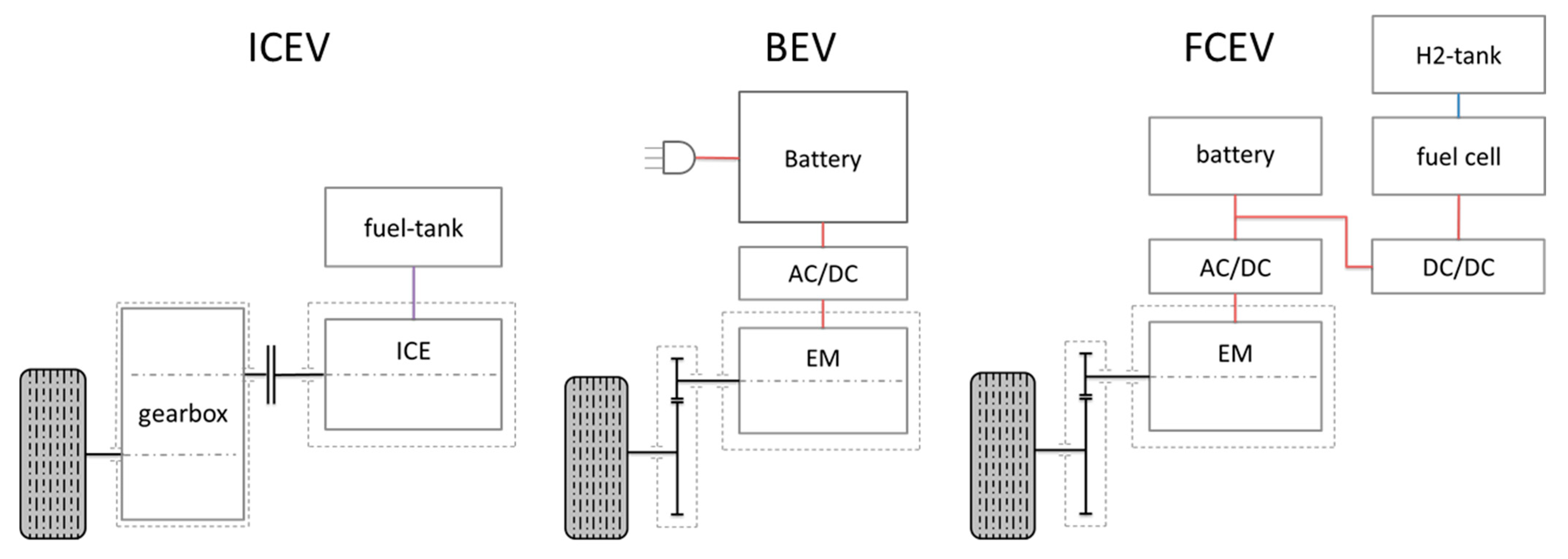
With regard to alternative powertrains in [8], the performance parameters; working principles; and recent developments of ICEVs, battery-only vehicles (BEVs), and (fuel cell vehicles) FCEVs were compared. The current advantages and disadvantages were also summarized. It was concluded that there will be no single strategy for the different heavy-duty applications and that it is important to understand more about the different powertrain options. The authors of [9] noted that, unlike road passenger transport, road freight transport still lacks marketable products. For Germany in particular, it is still unclear which boundary conditions (e.g., subsidies and regulations) will be set for the various powertrain options.

In order to better classify these various drive options, evaluations were carried out in various studies with regard to economy, efficiency, and emissions. In [10], a total-cost-of-ownership (TCO) analysis for the time range till 2030 was made for heavy-duty BEVs and compared with the conventional ICE. For this purpose, a model was created that defines various transport relations for which the costs were determined individually. Energy consumption is calculated on the basis of constant consumption values per powertrain option multiplied by the mileage for a relation. The extra weight for batteries as well as the auxiliary power consumers are not considered. This model was enhanced in [9], where heavy-duty FCEVs and BEVs with catenary have also been evaluated. In addition, the model was extended to include the calculation of CO₂ emissions for operation and production. A similar approach to making TCO estimation was followed in [4] but without distinguishing between different transport relations.

A deeper investigation with a detailed model of the powertrain was carried out in [11]. In this paper, only heavy-duty BEVs were considered. The focus is on the range of BEVs with different variants of batteries and motors. This model was extended to heavy FCEVs in [12]. In this study, BEVs, FCEVs, and ICEVs were also compared. This comparison was based on energy consumption from tank-to-wheel, i.e., the energy that has to be put into the vehicle. This method neglects the efficiency losses that occur before the tank, e.g., in the production of the fuel (diesel, hydrogen) or electricity.

When comparing different energy sources such as electricity and different fuels, it is not sufficient to compare energy consumption based on the tank-to-wheel efficiency. It is necessary to consider all efficiencies in the whole energy chain. An approach to implementing primary energy efficiencies in the energy calculation for different powertrain options was introduced in [13]. In this paper, constant overall efficiencies were used for the different powertrain options, which are not dependent on the different applications. As the paper dates back to 2001, the data are also no longer up to date. The authors of [4] had a similar approach to calculating the primary energy consumption of BEVs, FCEVs, and ICEVs with fuel from power-to-liquid and power-to-methane production. This was also not carried out for a certain application. Instead, it was assumed that the entire transport volume in Germany for heavy vehicles weighing more than 26 tons would be handled with one of the above-mentioned powertrain options. It was also assumed that only renewable electricity is used as a base for the production of fuels (in the case of hydrogen, electrolysis is assumed).

When it comes to economics, some TCO analyses have already been introduced above. In [14], the expected fuel price for hydrogen in the next decade and the price required to break even in different EU countries were investigated and compared to BEVs and ICEVs.

The effect of autonomous vehicles on the energy consumption of the transport sector has already been investigated in several studies [15,16,17]. These studies investigate how energy consumption changes as a result of changing travel demand as well as an optimized route planning of connected vehicles. They do not evaluate how the energy consumption of an autonomous vehicle changes compared with a conventional vehicle when driving the same scenario.

This research also serves as preliminary work for a long-haul robot truck (LHRT) concept development within the framework of the DLR project “VMo4Orte” [18]. For this purpose, it is to be investigated which powertrain concept is best suited for the most used operating variants in current road transport in the EU. The focus is especially on hub-to-hub logistic traffic. The LHRT concept will be evaluated later on based on a corresponding real-world transport scenario. In addition to full automation, suitable powertrains are also being investigated and compared in the LHRT concept. Another autonomous vehicle concept with a mover with a changeable capsule for different transport applications has already been evaluated in previous work [19]. Therefore, BEV, FCEV, and ICEV powertrains are being simulated in the Dymola modeling environment in a standard cycle and a daily driving cycle so that the results can then be compared and evaluated in terms of primary energy consumption, CO₂ emissions, and energy benefits for autonomous driving. This modeling environment is currently developed and applied in the DLR projects “FFAE” and “V&V4NGC” [20].

The contribution of this paper is the development of a method to determine the CO₂ emissions, primary energy consumption, and fuel costs for different powertrain options that can be applied on different applications and scenarios. This method includes detailed and dynamic models of different powertrains, including a model for the auxiliaries including the cabin climatization. Using these models, different applications and scenarios based on the velocity and gradient profiles can be evaluated in detail and compared against each other to evaluate which powertrain option fits best to a certain application. The evaluation considers the primary energy consumption instead of the tank-to-wheel evaluation to compare different energy sources. CO₂ emissions have been investigated using current and estimated CO₂ emissions. The economic evaluation was performed regarding fuel costs. The cab model was used to investigate whether omitting the cabin and other driver-related auxiliaries leads to lower energy consumption in autonomous vehicles.

The paper is structured as follows. In Section 2.1, a vehicle use case is defined, defining the type and the size of the vehicles. In Section 2.2, two typical scenarios for this vehicle use case are developed. The parametrization of the vehicles is determined in Section 2.3. The powertrain design is needed as an input to the simulation, so a powertrain design is created in Section 2.4. 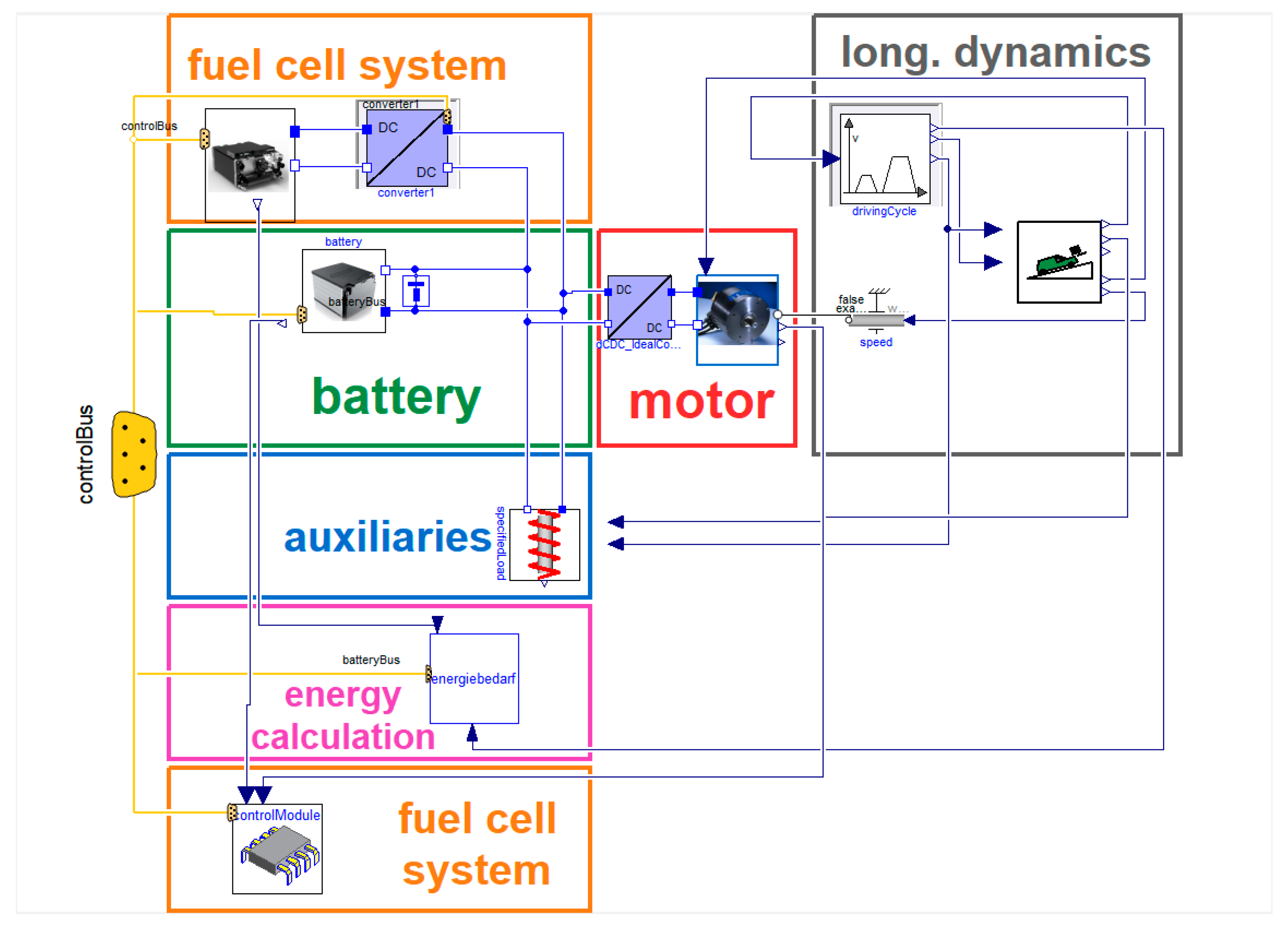The simulations that are performed are described in Section 2.5. The simulation model is then introduced in Section 2.6. A postprocessed method to calculate the primary energy consumption, CO₂ emission, and fuel costs is presented in Section 2.7. In Section 3, the results are presented, divided up into the two scenarios, as well as autonomous driving. Finally, the discussion is provided in Section 4.

2. Materials and Methods

2.1. Vehicle Use Case

In the first step, a vehicle use case is defined. For this, it has to be defined which vehicle type is being considered. In the Commission Regulation (EU) 2017/2400, vehicles are grouped into 17 different vehicle groups. They are distinguished on the basis of the following parameters: chassis configuration, axle configuration, and permissible gross weight. In [21], the CO₂ emissions and sales shares of these 17 vehicle groups are determined. It can be seen that the fifth vehicle group accounts for the largest share of CO₂ emissions, at over 50%. It is also the vehicle group with the highest proportion of vehicles sold, at 43%. The fifth vehicle group represents 4 × 2 tractors with a weight of over 16 tons, which is used here as the use case.

To complete the use case, a trailer type is also defined. In [22], it is evident that the combination of a three-axle semitrailer with a 4 × 2 tractor is the most common. Therefore, this combination is chosen for the use case.

Comparing fully autonomous HDVs with conventional, driver-controlled vehicles, it is clear that the most significant difference is the elimination of the driver’s cab. This means that various driver-related auxiliary consumers such as information systems or air conditioning/ventilation systems can be omitted. Instead, additional sensor technology is needed to enable autonomous driving. Following previous work by DLR with the autonomous mover concept “U-Shift”, an additional electrical power requirement of 2500 W for the sensors and associated control units is assumed [19].

Depending on the architecture of the powertrain, the vehicles differ in terms of weight. As reference, a Mercedes-Benz Actros 4 × 2 heavy-duty truck is used. This vehicle has an ICEV powertrain and is combined with a flatbed semitrailer to determine the weight. The weight of the Actros is 6867 kg [23]. A typical ICEV powertrain weighs 3000 kg [24], which gives a weight of the chassis of 3867 kg. A typical empty trailer has a weight of 7000 kg [21]. For the different powertrain topologies, the weights of the corresponding powertrain components are added to obtain the curb weight. These weights can be seen in

Table 1. Weight determination of the different vehicles.

Parameter	ICEV	BEV	FCEV
chassis tractor	3867 kg	3867 kg	3867 kg
+mechanical powertrain ICE	3000 kg
+battery		5887 kg	910 kg
+power electronics, e-motor		400 kg	400 kg
+fuel cell			125 kg
+hydrogen tank			1275 kg
+trailer (empty)	7000 kg	7000 kg	7000 kg
=Curb weight	13,867 kg	17,154 kg	13,577 kg
Reference weight	40,000 kg	40,000 kg	40,000 kg
Maximum weight	40,000 kg	42,000 kg	42,000 kg
payload (max. weight − curb weight)	26,133 kg	24,846 kg	28,423 kg

. For the electric motor and power electronics, 400 kg is assumed [24]. The battery size of the BEV was determined by defining a battery energy content of 883 kWh (Lithium-NMC battery system), which is sufficient for a 600 km range in the later introduced daycycle. Moreover, this range derives from this daycycle. In the FCEV, a smaller battery with an energy content of 137 kWh was used, which is sufficient to cover power peaks that the fuel cell is unable to cover and allows the recuperation of traction power. The fuel cell has a maximum electric power of 190 kW. Using three hydrogen tanks, the FCEV can store 90 kg of hydrogen. This results in different curb weights, whereas the FCEV is the lightest and the BEV the heaviest. In the EU, emission-free trucks are allowed to have a maximum weight of 42,000 kg, with all other trucks allowed only 40,000 kg (in cross-border transport) [25]. To enable a technical comparison between all three powertrain topologies at the same vehicle weight, a reference weight of 40,000 kg was introduced for all three variants. Calculating the difference between the maximum weight and the curb weight results in the payload, showing that the FCEV has the highest payload and the BEV has the lowest.

2.2. Driving Cycle Determination

Two different cycles are used to simulate the powertrain. The first is a standard cycle called the FIGE cycle, also known as the ETC cycle. This cycle is based on real driving data. This cycle was also used to validate the CO₂ emissions calculation of the VECTO-Tool [26]. The longitudinal vehicle velocity profile is shown in Figure 1. The original cycle accelerates the vehicle up to velocities of 90 km/h. In Germany, only speeds of 80 km/h are allowed on motorways. Hence, this cycle was adjusted to maintain the maximum allowed velocity. In addition, at the end of the cycle, the deceleration is limited to typical values. The cycle consists of three parts designed to represent traffic in urban and rural areas and on motorways. Each part has a temporal length of 600 s.

The second cycle was newly created and is composed of the three parts of the FIGE cycle. This cycle should represent a full-day truck trip consisting of a transportation relationship between two hubs and a driver break time. This cycle is referred as a daycycle and the velocity profile is visualized in Figure 2. A total of 581 km is driven in this cycle in a time of 10:15 h. This cycle consists of different sections for urban and rural transportation (transfer to motorway) (blue underline), hub loading and unloading time (red underline), motorway (yellow underline), and driver braking time (green underline).

Based on this, a daycycle was created, which is composed of the three parts of the FIGE cycle (urban, rural, motorway). This cycle is called a daycycle and should represent a typical journey of an HDV during a whole day. The velocity profile of this cycle is shown in Figure 2. The created daily cycle covers a distance of 581 km over a period of 10:15 h and is divided into several sections with transfer (urban and rural) parts (blue underline), loading and unloading times (red underline), motorway parts (yellow underline), and break times (green underline). The first and last sections of the vehicle drive empty with its curb weight. After the loading procedure, the vehicle has the reference or maximum weight until the unloading procedure. Thus, of the 9 h driving time, 2:20 h are driven without payload, which corresponds to a share of 25.8%.

2.3. Vehicle Parametrisation

Auxiliary power consumers are investigated if they can be omitted in an autonomous vehicle and it is determined which of them are still necessary. An overview on the auxiliary consumers’ average power is provided in

Table 2. Average power of the auxiliary consumers of the vehicles.

Auxiliary Consumers	Vehicle with Driver Cabin [W]	Vehicle without Driver Cabin [W]
radio	20	-
instrument lighting	20	-
heated windshield	60	-
electric heating	1000	-
electric air conditioner compressor max. power	(3000)	-
parking light	7	7
low beam	90	90
turn signal light	90	90
windscreen wiper	10	10
license plate light	25	25
brake light	11	11
fog light	20	20
rear fog light	2	2
turn signal	5	5
electric power steering pump	1800	1800
electric air compressor	4500	4500
power of sensors	-	2500
total	7660–9660	9060

. These values are derived from [27]. As the air conditioning (AC) and heating unit are simulated in the model, a reference value was added for information. In particular, for the AC compressor, the maximum value was given because the average value is based on usage.

To calculate the mechanical traction force at the wheel, the vehicle longitudinal dynamics, including rolling resistance, air resistance, and acceleration resistance, were considered. The necessary values are listed in

Table 3. Resistance parameters of the vehicles.

Description	Character	Unit	Value
Vehicle mass	mv	[kg]	42,000
Gravitational acceleration	g	[m/s2]	9.81
Rolling resistance coefficient	cr	[-]	0.006
Drag coefficient cabin vehicle	cw	[-]	0.6
Drag coefficient autonomous vehicle	cw	[-]	0.52
Front face	Af	[m2]	9.615
Air density	ρ	[kg/m3]	1.2041

. Using several references, an average value of 0.6 was found for the air drag coefficient (c_w) of vehicles with a cabin. Vehicles without cabin have a lower drag coefficient; according to [21], a value of 0.52 was assumed. The density of air 𝜌 is assumed to be 1.2041 kg/m³, given for the altitude at sea level (0 m) and an ambient temperature of 20 °C. Considering the frontal area of the visible tires and the main body of the vehicle, the cross-sectional area A_f was determined to be 9.615 m².

For the calculation of the acceleration resistance, the rotating masses of the vehicle are included by the rotating mass factor e, which is dependent on the vehicle mass and varies in the following simulations from 1.036 to 1.112.

The climatization of the driver’s cabin is simulated in two different climatic scenarios, which should represent cooling in summer and heating in winter. The cooling of the cabin is carried out by an air conditioning system (AC), while the heating is performed by an electric heater in the case of the BEV and FCEV. For the ICEV, only the cooling scenario was considered, as waste heat from the ICE is used to heat the cabin, so there is no additional energy consumption. The ambient conditions for the scenarios are provided in

Table 4. Parameters for the climatic scenarios.

Parameter	Unit	Heating	Cooling
temperature cabin	[°C]	22.00	22.00
ambient temperature	[°C]	3.78	26.49
ambient humidity	[%]	72.48	46.80
solar radiation constant	[Wm2]	134.16	524.87

. This dataset comes from [28] and should represent typical heating and cooling scenarios in Europe.

2.4. Powertrain Design

For the parametrization of the simulation model, the BEV and FCEV powertrain had to be designed to determine the size of the motors and the mechanical drivetrain components. For the ICEV, the values from the reference vehicle Actros are used. To calculate the mechanical traction force needed, the following equations are used. The data are taken from Table 3. The rolling resistance F_r is calculated with Equation (1). The air drag resistance F_air is determined with Equation (2), where v is the vehicle velocity. The inclination resistance depends on the inclination angle α and is given in Equation (3). These three equations determine the resistance force that must be overcome when driving at a constant velocity. For the vehicle to accelerate, the acceleration resistance is given by the vehicle acceleration, a, in Equation (3).

F_r = c_rm_vgcos(α)

(1)

F_air = 0.5ρA_fc_wv²

(2)

F_g = m_vgsin(α)

(3)

F_a = m_vae

(4)

In Germany, gradients of up to 6% can occur on highways [29]. A maximum velocity of 80 km/h was assumed. This yields a maximum resistance force of 29 kN and a necessary power of 636 kW. An electric motor from BRUSA Elektronik AG (Buchs, Switzerland), the HSM1-10.18.22., was selected as the motor. This motor must be installed four times, which yields a power of 840 kW. This motor thus generates sufficient torque to achieve the required speeds in the selected drive cycles and has sufficient reserves for acceleration. The Actros OM470 combustion engine from Mercedes (Stuttgart, Germany) is used for the ICE vehicle.

2.5. Simulation Concept

According to Table 1, the vehicle models for the BEV and FCEV are thus parametrized with two different weights and the ICEV model with one weight. BEV and FCEV are additionally distinguished between autonomous vehicles and conventional vehicles with a driver. The BEV and FCEV with a driver are also distinguished between heating and cooling scenarios, as given in Table 4. The simulation concept is shown in

Table 5. Simulation concept with the different parameter sets.

Powertrain	Weight	Steering Type	Cabin
BEV	reference weight	autonomous	-
		driver	heating
			cooling
	maximum weight	autonomous	-
		driver	heating
			cooling
FCEV	reference weight	autonomous	-
		driver	heating
			cooling
	maximum weight	autonomous	-
		driver	heating
			cooling
ICEV	maximum weight = reference weight	driver	cooling

. Each parameter set is applied twice, once in both driving cycles. It has to be added that, for the daycycle, the curb weight is also used for the corresponding sections.

2.6. Modelling

The modeled topologies of the three powertrain topologies are visualized in Figure 3. This visualization includes the ICE, the electric motor (EM), the traction inverter (AC/DC), the DC-to-DC converter (DC/DC), the traction battery, the fuel cell, the hydrogen (H2) tank, the fuel-tank for diesel, and a gearbox. Mechanical power transmission is marked with black lines, electrical power transmission with red lines, hydrogen flow with a blue line, and diesel flow with a purple line.

Using the system simulation tool Dymola, which is based on the Modelica language, a modular approach was used to develop these models. There have already been model libraries made by the DLR; for example, the alternative vehicles library that can be used to simulate alternative powertrains as well as ICEVs [30]. For the ICEV, an existing ICEV model was used from the alternative vehicles library.

For the BEV and FCEV, a new vehicle simulation library was used, derived from the alternative vehicles library. These models focus on the energy consumption calculation. A BEV model already existed from previous work [31]. Integrating a fuel cell system with a DC-to-DC converter and a control module, this model was extended to a FCEV model. The system (top) level of this model can be seen in Figure 4. This model consists of a fuel cell system with a control module (orange), a battery system with a DC link (green), the auxiliaries including a cabin model (blue), an electric motor model with a traction inverter (red), the longitudinal dynamics including the drive cycle (grey), and a block for the energy calculation (magenta). The longitudinal dynamics were modeled using Equations (1)–(4). The speed and gradient profile of different driving cycles can be used as input. The fuel cell system, the battery system, the electric motor, and the power electronics are modeled using characteristic diagrams. The auxiliaries are modeled using the average values from Table 2 and include a cabin model, which integrates both heating and AC. This model is derived from the approach in [32]. With this model, the differences in energy consumption for autonomous vehicles and vehicles with a cabin are investigated. This model assumes a constant certain temperature inside the cabin and calculates the thermal as well as electrical power needed to maintain this temperature. This electrical power is then given to the vehicle model. In this model, the cabin is modeled as a 1D mass. For the calculation of the heat transfer, the thermal resistances of the vehicle body and the vehicle windows, as well as the thermal radiation and solar radiation, are considered. A straightforward model of the AC system and the heating system calculates the electrical power from the thermal power. For autonomous vehicles, the cabin model is replaced by the auxiliary demand of the autonomous driving functions, which is a constant power demand. This modular model makes it easy to adapt new powertrain options and technologies. It is also easy to implement other scenarios and vehicle parameters.

The plausibility of the model was checked by comparing the model results of the electricity, hydrogen, and diesel consumption for certain scenarios with references from the literature. Static operating point simulations were also performed and compared with the results from the corresponding equations.

2.7. Method for the Calculation of Primary Energy, CO₂ Emissions, and Fuel Costs

The electrical energy consumption for the BEV was determined by measuring and integrating the electrical power at the battery terminal P_Batt according to Equation (6). For the FCEV and ICEV, the specific energy contents of the consumed fuel (hydrogen or diesel) according to Equations (5) and (7) are used. For this, the heating value of hydrogen e_hydrogen with 33.33 kWh/kg or diesel e_diesel with 9.8 kWh/L is used.

$${\mathrm{E}}_{\mathrm{ICEV}}={\displaystyle \int }{\dot{\mathrm{V}}}_{\mathrm{diesel}}{\mathrm{e}}_{\mathrm{diesel}} \mathrm{dt}$$

(5)

$${\mathrm{E}}_{\mathrm{BEV}}={\displaystyle \int }{\mathrm{P}}_{\mathrm{Batt}} \mathrm{dt}$$

(6)

$${\mathrm{E}}_{\mathrm{FCEV}}={\displaystyle \int }{\dot{\mathrm{m}}}_{\mathrm{hydrogen}}{\mathrm{e}}_{\mathrm{hydrogen}} \mathrm{dt}$$

(7)

The primary energy consumption is determined using primary energy factors (PFs) for electricity, hydrogen, and diesel. The primary energy factors include the energy consumption needed for the transformation of primary energy (such as oil, gas, and the sun) via secondary energy (e.g., heating oil or briquettes) to end energy (e.g., fuels and electricity) and, therefore, include the transformation losses [33]. As more and more renewable energy sources are incorporated into power generation, the primary energy factor becomes smaller. This was already observed in [34] for countries of the EU by analyzing different statistics and comparing different calculation methods. For this article, the primary energy factors in

Table 6. Primary energy factors.

End Energy Source	Primary Energy Factor	Source
diesel	1.22	[35]
electricity low PF	2.1	[34]
electricity high PF	2.5	[34]
hydrogen	1.46	[33]

are used. For electricity generation, two different PFs are designated—a lower one that represents the PF in the EU at the moment and a higher one that represents the current PF in Germany. This should show the sensitivity of the energy consumption results to the ways in which electricity is produced and the extent of the difference in primary energy consumption of BEVs in different countries. For hydrogen, it is assumed that it is made by steam reforming of natural gas in Germany without CO₂ capture.

For fuel costs, the fuel prices in

Table 7. Fuel prices.

End Energy Source	Fuel Price	Source
diesel	1.59 €/L	[36]
electricity	0.3994 €/kWh	[37]
hydrogen	12.85 €/kg	[38]

were assumed. The diesel price was the average price in Germany in June 2023. For electricity, the average price was assumed based on 12 July 2023. The hydrogen price was assumed for trucks with 350-bar hydrogen pressure in Germany.

The CO₂ emissions for electrified powertrains are dependent on the way in which the electricity and hydrogen are generated/produced. It was thus decided to define two scenarios. The first scenario represents the current electricity mix inside the EU and the hydrogen made by steam reforming of natural gas. The second scenario represents a future electricity mix with renewable energy sources and hydrogen made by electrolysis with this electricity mix. To determine the CO₂ emissions, the CO₂ emission factors in

Table 8. CO₂ emission factors.

End Energy Source	Current CO2 Emissions	Source	Future CO2 Emissions	Source
diesel	0.524 kg/L	[39]	0.524 kg/L	[39]
electricity	0.238 kg/kWh	[40]	0.015 kg/kWh	[39]
hydrogen	0.289 kg/kWh	[33]	0.021 kg/kWh	[39]

are used and multiplied with the energy consumption of the different powertrain options.

3. Results

In this section, the simulation results are evaluated regarding the primary energy consumption, CO₂ emissions, and fuel costs. The results from the FIGE cycle are used to analyze the differences in different road types (urban, rural, and motorway) and to evaluate the energy consumption for different application scenarios. With the results from the daycycle, the CO₂ emissions and fuel costs are determined for a realistic scenario.

3.1. FIGE Cycle

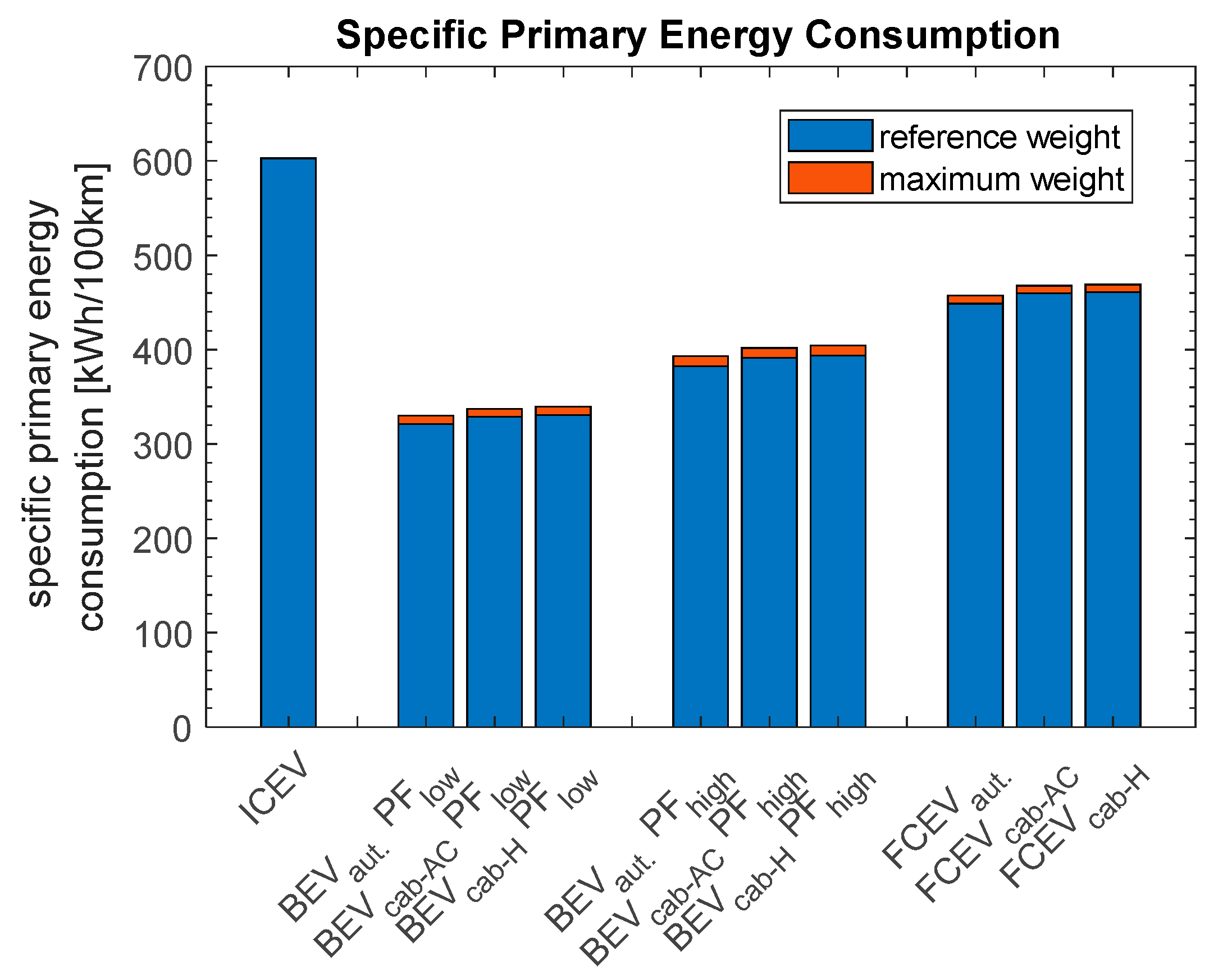
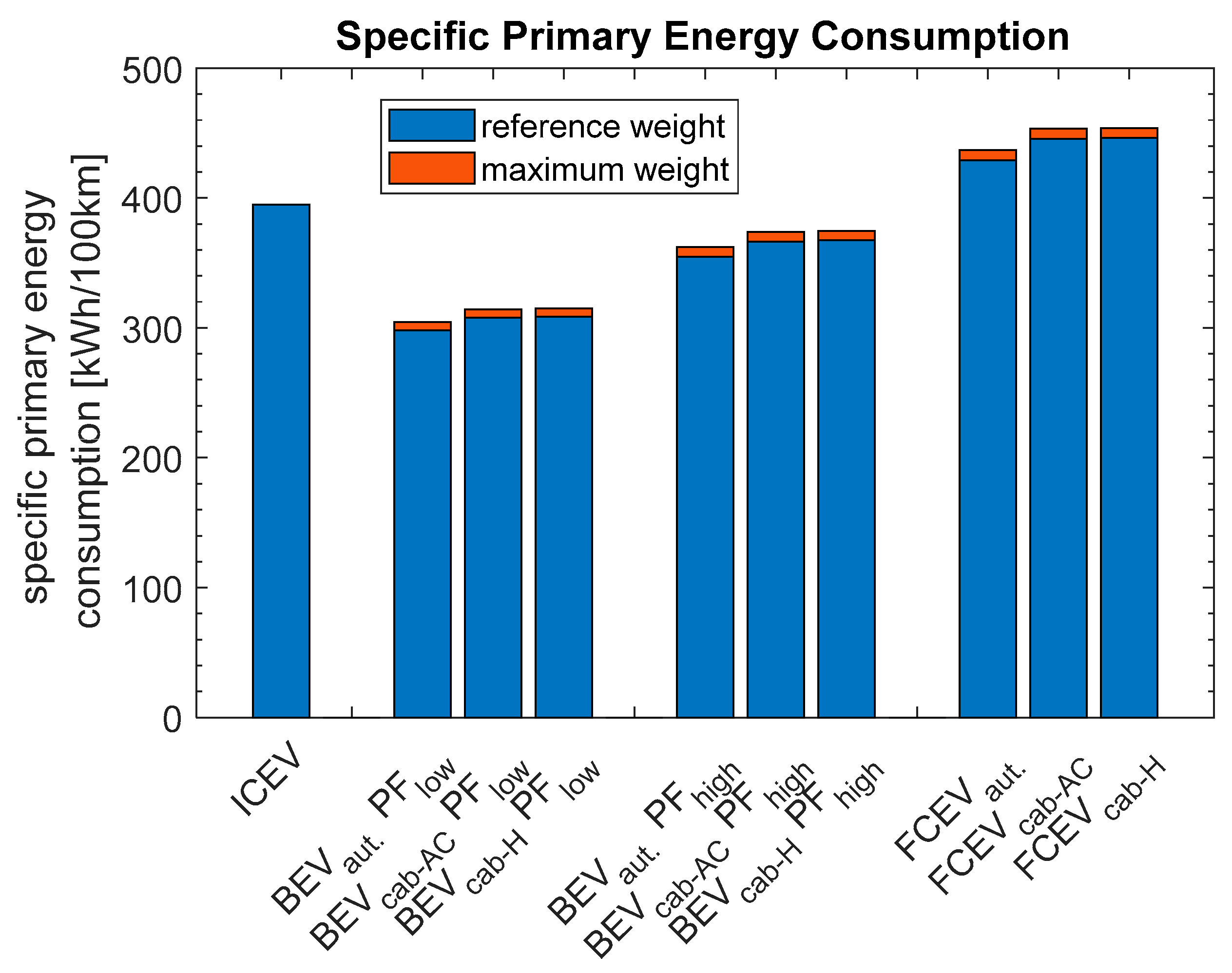
In Figure 5, the specific primary energy consumption for the different powertrain topologies (ICEV, BEV, and FCEV) is shown. It is distinguished between the reference weight (40 tons for all vehicles) and the maximum weight, which is 2 tons higher for the electrified vehicles. For the BEV, it is also distinguished between the high and low primary energy factors for electricity.

It becomes clear that the ICEV has the highest specific primary energy consumption, followed by the FCEV and then the BEV. The variation in the primary energy factor for the BEV leads to high sensitivity. While the primary energy factor for diesel will remain the same in the future, the factors for electricity and hydrogen will decrease in the coming years because of the upcoming use of renewable energy sources to generate electricity and the combination of renewable energy electricity and electrolysis to generate hydrogen. Consequently, it is expected that, for electrified powertrains, the primary energy consumption will also decrease the coming years. Autonomous vehicles can reduce energy consumption by up to 10 kWh/100 km compared with vehicles with a cabin.

The most important benefit factor for the user is the achievable payload, which differs for the different powertrain variants. To take this into account, the specific primary energy consumption is divided by the payload to obtain the energy value needed per ton of payload. The results are shown in Figure 6. For this consideration, the maximum weight yields lower energy consumption quotients because the resulting payload is higher.

As before, the ICEV has the highest energy consumption, followed by the FCEV and BEV. However, it is clear that the gap between the BEV and FCEV is becoming smaller. For the BEVs with a higher PF, the energy consumption is almost the same because of the benefit of a higher payload for the FCEVs.

A closer look at the results shows that the characteristics of the different parts of the FIGE cycle (urban, rural, and motorway) are very different. In Figure 7, the charged and discharged energy shares for the battery in the FIGE cycle (one-third of the cycle each) for the BEV are visualized. In case of the BEV, charged energy means recuperated energy from electrical braking, whereas discharged energy means energy for traction and auxiliaries.

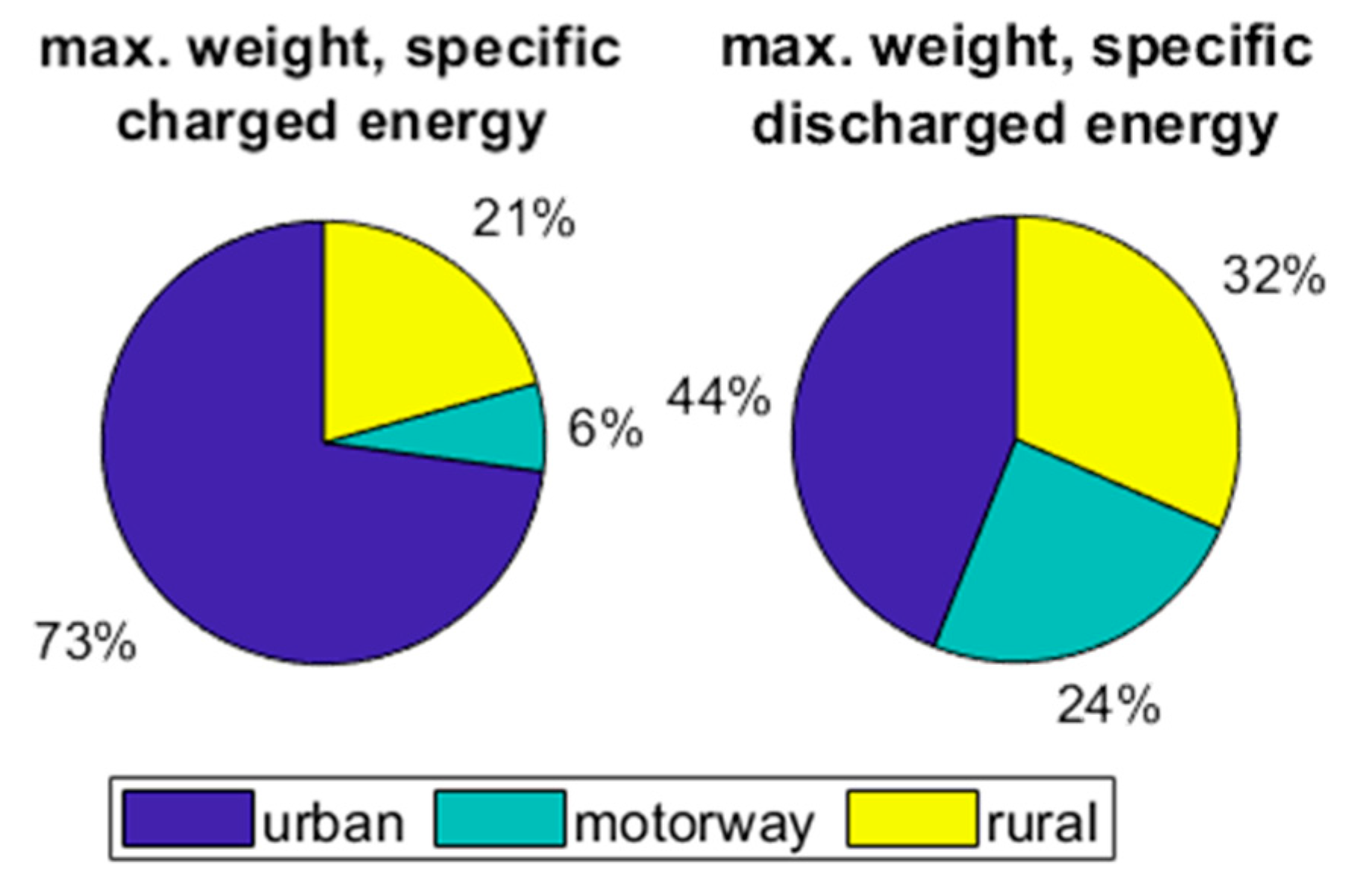
It becomes clear that more energy can be recuperated in the urban and rural part than on motorways. This is because of the higher incidence of acceleration and deceleration operations. On the other hand, the motorway and rural part are responsible for 79% of the energy demand owing to the higher velocity. It should be mentioned that, in total, the charged energy is around 22% of the charged energy for the whole FIGE cycle, so 22% of the energy needed could be recuperated by an electrified powertrain. If the energy consumption is referred to as 100 km as a basis, the shares shift as seen in Figure 8.

Still, the charged energy share for the urban part is the greatest. Looking at the discharged energy, it can be seen that the urban part has the highest share. This is because of the high incidence of accelerations and the lower mileage, so more energy is needed to overcome the same distance in urban areas than in rural areas or on the motorway. Moreover, the power of the auxiliaries is dependent on the time and not on the mileage. If the vehicle is in standstill or a low velocity in urban areas, the auxiliaries need the same power as on the motorway with a high velocity, so, per 100 km, the specific energy consumption for the auxiliaries is higher in the urban part.

The specific primary energy consumptions in the different parts of the FIGE cycle are additionally compared for each powertrain architecture in Figure 9. For the BEV and FCEV, the cabin vehicle with the cooling scenario is used.

The greatest difference between the three parts is given for the ICEVs. In the urban part, the primary energy consumption is more than twice as much as in the rural part and more than four times higher than in the urban part. The main reasons are that the ICEV is not able to recuperate energy with electrical braking and, as shown in Figure 7 and Figure 8, especially in the urban part, the vehicle could recuperate energy. The overall efficiency of the ICEV is also low in urban areas, ranging from 5% (empty vehicle) to 16% (full vehicle) in the simulations. It is noticeable that, for the urban part, the ICEV has the same specific energy consumption as the BEV with a low PF and less specific energy consumption than the BEV with a high PF and the FCEV.

3.2. Daycycle

The results in the daycycle differ from those in the FIGE cycle, as the daycycle mainly consists of motorway parts. Analogous to Figure 5, the specific primary energy consumption for the different powertrain topologies is shown in Figure 10. It is also distinguished between the reference weight and the maximum weight. The primary energy consumption for the FCEVs is the highest, followed by the ICEV and then the BEV. Compared with the results in the FIGE cycle, the high percentage of highway passages in the daily cycle gives the ICEV the opportunity to not have the highest energy consumption. However, regarding the results of the BEV with both PFs, it becomes obvious that the results are sensitive to the way in which the electricity/hydrogen is generated/produced. As the PF of diesel will not change in the future, the PF of electricity and hydrogen does change. It can also be concluded that the primary energy consumption of electrified powertrains will decrease with succeeding expansion of renewable energy sources. Autonomous vehicles have a lower specific primary energy consumption of 11 kWh/100 km for the BEV and 17 kWh/100 km for the FCEV.

Considering the payload, the results change. Analogous to Figure 6, in Figure 11, the specific primary energy consumption per ton of payload for the daycycle is shown. Again, the maximum weight yields lower values for the electrified powertrains compared with the reference weight.

As the payload for the FCEV is the highest and the payload for the BEV is the lowest for the three vehicles, the specific primary energy consumption for the FCEV, the BEV with a high PF, and the ICEV is now in the same range. With a low PF, the BEV has still the lowest values.

The CO₂ emissions are regarded in the above-mentioned two scenarios. The results for the first scenario for the daycycle are shown in Figure 12.

The CO₂ emissions for the ICEV are the highest. With the current hydrogen made by steam reforming, the FCEV has 2.5 times higher CO₂ emissions than the BEV. It should be noted that the CO₂ emission factor for electricity is decreasing every year at the moment, and differs significantly among different countries of the EU. For the second scenario, the CO₂ emissions for the daycycle are shown in Figure 13.

It is obvious that, in this scenario, the CO₂ emissions of the ICEV are about 31 times higher than those of the BEV and 16 times higher than those of the FCEV in the daily cycle.

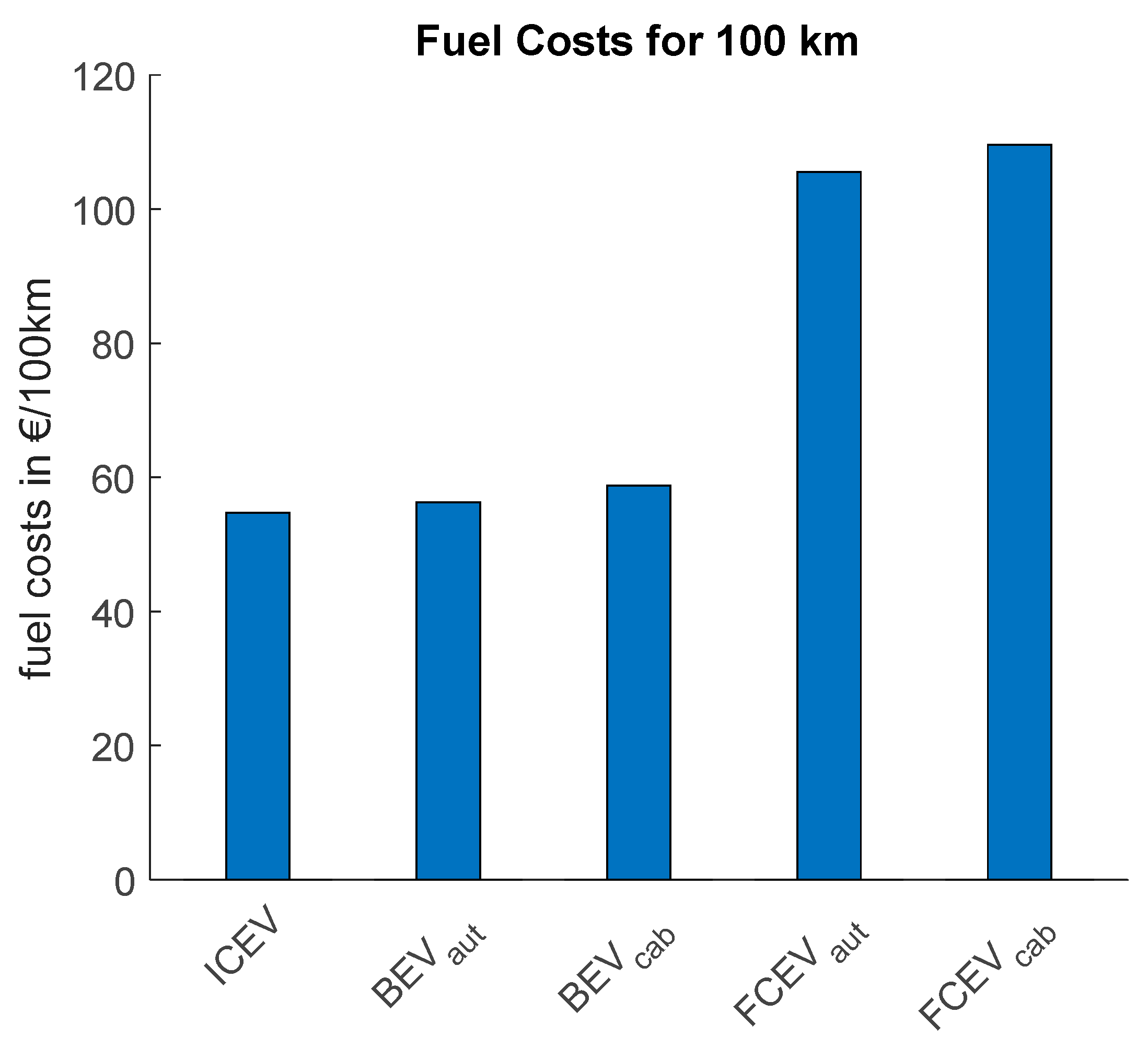
In Figure 14, the fuel costs for a 100 km distance based on the daycycle are visualized for the different powertrain topologies.

The ICEV has the lowest fuel costs, followed directly by the BEV. It should be noted that the basis for electricity is the standard electricity price. Buying electricity at public charging points is more expensive. The FCEV has the highest fuel costs owing to the high hydrogen price at the moment. To achieve competitive conditions for the FCEV in terms of fuel costs, the price of hydrogen must be at least halved. In [14], the price of green hydrogen at the pump in 2035 for several European countries was estimated to be between 5.5 €/kg (Poland) and 8.1 €/kg (Germany). This price is made up of the production costs of green hydrogen and the costs for the fueling station. This study also assumed an increasing diesel price in the future.

3.3. Autonomous Driving

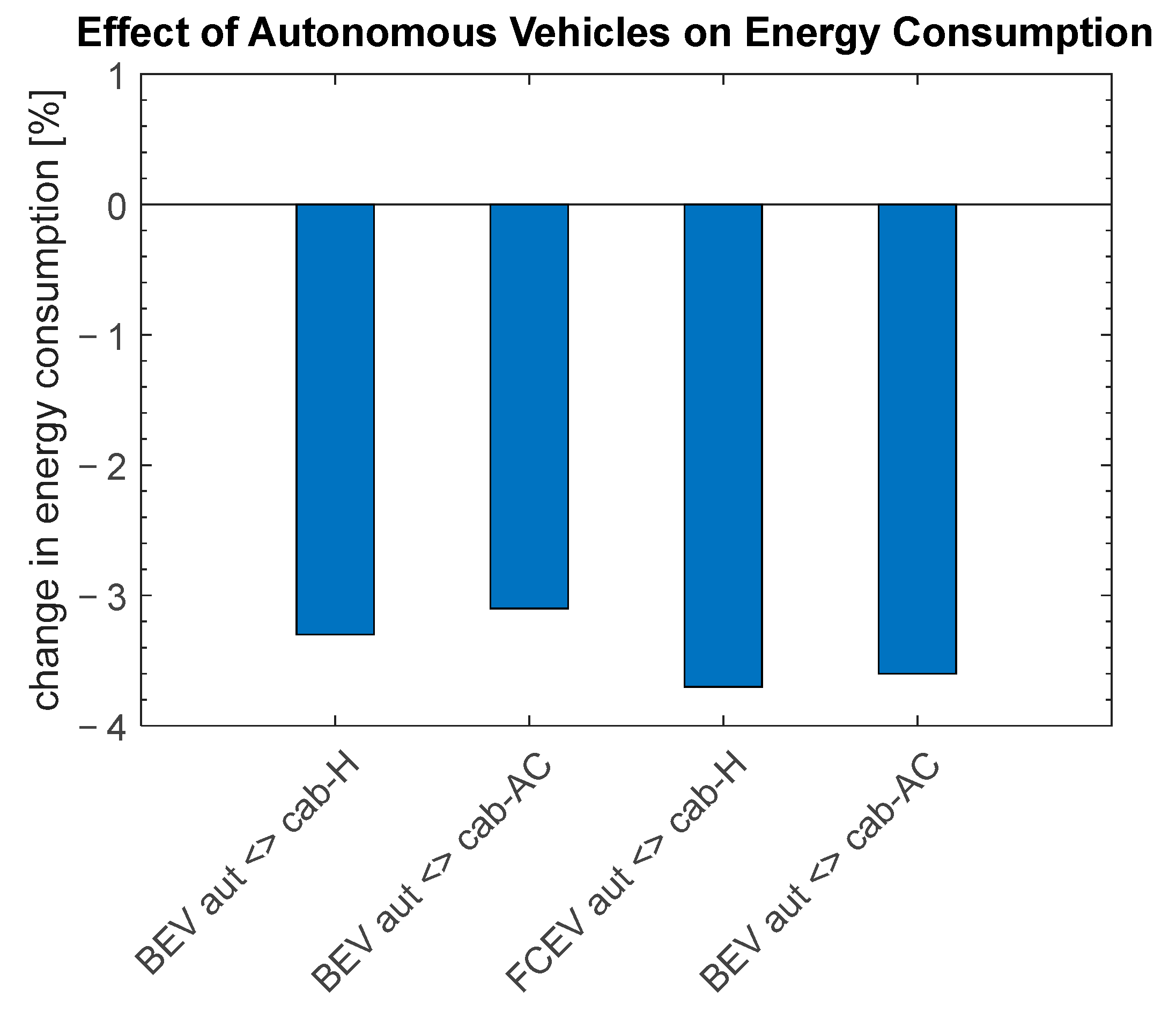
A key question of this article is whether autonomous driving has an increasing or decreasing effect on energy consumption. In Figure 5 and Figure 10, it is already visible that autonomous driving can reduce the energy consumption in the FIGE cycle and the daycycle. In Figure 15, the primary energy consumption in the daycycle of the autonomous vehicle is directly compared with the cabin vehicles in both climatic scenarios on a percentage basis.

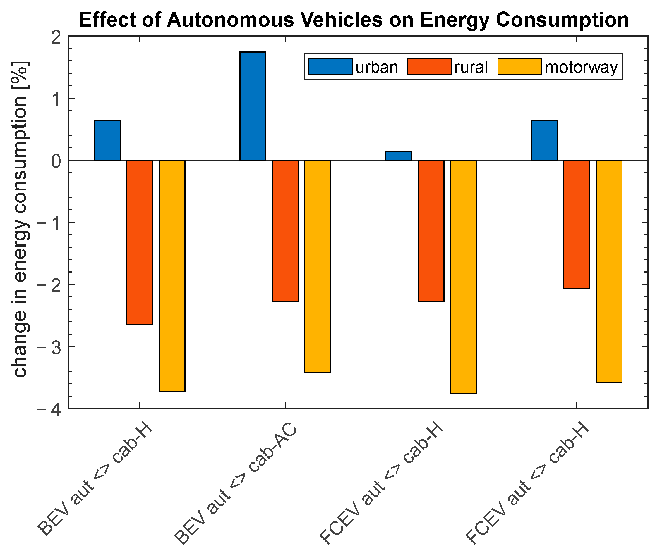
It is obvious that the autonomous vehicles can reduce the energy consumption by up to 3.7% in the daycycle. In Figure 16, the effect of autonomous driving on the primary energy consumption is shown for the different parts of the FIGE cycle. Here, the autonomous vehicle is directly compared to the cabin vehicles in both climatic scenarios on a percentage basis.

For the rural and motorway parts, the energy consumption for the autonomous vehicle is still lower than for the cabin vehicles. However, for the urban part, the autonomous vehicle needs more energy than the cabin vehicle. This yields the assumption that the energy reduction is mainly caused by the lower air drag coefficient of autonomous vehicles. The air drag coefficient determines the air resistance as a function of the squared longitudinal velocity. Hence, the higher velocities in the rural and motorway part yield higher energy reductions when lowering the air drag coefficient. This assumption was proven by simulations. Therefore, an autonomous FCEV with a reference weight was simulated with an air drag coefficient of 0.6 instead of 0.52 for both the FIGE cycle and the daily cycle. For the FIGE cycle, the primary energy consumption was 316.6 kWh/100 km instead of 307.3 kWh/100 km. This value is 1.9 kWh/100 km higher than for the cooling scenario and 1.0 kWh/100 km higher than for the heating scenario. For the daycycle, the new simulation resulted in 306.8 kWh/100 km, which is 1.6 kWh/100 km and 1.2 kWh/100 km higher than the cooling and heating scenarios, respectively. This shows that the assumption was correct, and the main energy reduction potential for this use case of autonomous vehicles comes from the improvement in the air drag coefficient, based on the above-made assumptions.

4. Discussion

As assumed from [13], using BEVs and FCEVs can help reduce primary energy consumption from heavy-duty vehicles, whereas BEVs are supposed to have the lowest primary energy consumption. However, this depends heavily on the way in which electricity or hydrogen is generated, which could be seen in this paper by using different primary energy factors. This also depends on how the BEVs or FCEVs are used in certain applications and scenarios. The impacts of different scenarios and road types on the energy consumption and the efficiencies are examined in this paper in detail using detailed models and different scenarios and road types. Another new finding is that FCEVs have the highest payload, but, because hydrogen production is currently non-renewable, primary energy consumption is even higher than for ICEVs in some scenarios, especially in the daycycle or on motorways. BEVs have the disadvantage of a lower payload; this is also included in this method by relating primary energy consumption to payload. Considering this as a result, the specific primary energy consumption of FCEVs and BEVs is already in a similar range in some cases.

The CO₂ emissions of the BEV and FCEV are lower than those of the ICEV, whereas the BEV has the lowest CO₂ emissions. This was also observed in [9]. However, as more and more electricity is generated from renewable sources, CO₂ emissions as well as primary energy consumption fall in the short term.

If hydrogen is produced by electrolysis with renewable electricity in the future, the primary energy consumption and CO₂ emissions for the FCEV will drop significantly. It turns out that ICEVs have lower efficiency due to the lack of recuperation capability, especially in urban areas. The ICEV instead has the lowest fuel cost, directly followed by the BEVs. Hydrogen is still expensive, as is driving FCEVs. Halving the fuel price for hydrogen could achieve the same fuel cost. In [14], it was found that the fuel price must be reduced to almost one-third to break-even. However, this study also includes a TCO analysis, which was not conducted in this paper. Even if using FCEVs is still expensive, they can foster sustainable development.

A method could be introduced that consists of modular models. They can easily be adapted to other technologies. The models can also be easily adapted to other scenarios. It is possible to investigate the energy efficiencies of different powertrain options and scenarios in detail. Moreover, a model for the auxiliaries was added.

Using this model, it was possible to evaluate that autonomous driving can reduce the energy consumption and, as a consequence, CO₂ emissions. Despite the original assumption, it turns out that the main reduction potential is the reduction in the air drag due to optimizations of the vehicle front and not omitting the cabin’s auxiliaries. In pure urban scenarios, autonomous driving yields even higher energy consumptions. However, autonomous vehicles also have additional exterior design options to further improve the energy consumption, which has already been evaluated in [18].

This study does not consider different driving behaviors of autonomous vehicles compared with conventional vehicles. Therefore, for example, for autonomous vehicles, it is not necessary to make a break, but the velocity can be reduced to reach the destination at the same time. For proper operation of autonomous vehicles, great efforts are being made to integrate sensors that collect and process environment information. Reducing the energy consumption of the sensors and related computational modules can improve the energy efficiency of autonomous vehicles. Works to improve the algorithms needed and to reduce computing complexity have already been performed in [41,42,43,44].

An additional aim of this study is to investigate a base operational scenario for the LHRT, using the FIGE cycle to evaluate the method. Additionally, a new cycle was introduced. This method can be applied to new real-world scenarios in the next step, such as hub-to-hub traffic.