Electrical Power Generation Forecasting from Renewable Energy Systems Using Artificial Intelligence Techniques

Abstract

Renewable energy (RE) sources, such as wind, geothermal, bioenergy, and solar, have gained interest in developed regions. The rapid expansion of the economies in the Middle East requires massive increases in electricity production capacity, and currently fossil fuel reserves meet most of the power station demand. There is a considerable measure of unpredictability surrounding the locations of the concerned regions where RE can be used to generate electricity. This makes forecasting difficult for the investor to estimate future electricity production that could be generated in each area over the course of a specific period. Energy production forecasting with complex time-series data is a challenge. However, artificial neural networks (ANNs) are well suited for handling nonlinearity effectively. This research aims to investigate the various ANN models capable of providing reliable predictions for sustainable sources of power such as wind and solar. In addition to the ANN models, a state-of-the-art ensemble learning approach is used to improve the accuracy of predictions further. The proposed strategies can forecast RE generation accurately over short and long time frames, relying on historical data for precise predictions. This work proposes a new hybrid ensemble framework that strategically combines multiple complementary machine learning (ML) models to improve RE forecasting accuracy. The ensemble learning (EL) methodology outperforms long short-term memory (LSTM), light gradient boosting machine (LightGBM), and sequenced-GRU in predicting wind power (MAE: 0.782, MAPE: 0.702, RMSE: 0.833) and solar power (MAE: 1.082, MAPE: 0.921, RMSE: 1.055). It achieved an impressive R² value of 0.9821, indicating its superior accuracy.

1. Introduction

The demand for renewable energy (RE) has surged due to fossil fuel pollution. The current primary concerns revolve around addressing increasing energy demands, ensuring stable power distribution, and minimizing emissions from non-renewable resources [1]. Optimizing sources of RE could significantly reduce greenhouse gas emissions and environmental degradation. The expanding industry has led to increased job opportunities in creating and implementing future RE solutions. The wide availability of sustainable energy contributes to lower energy costs, benefiting underdeveloped countries. Additionally, the environmentally friendly nature of REs, such wind and solar, has made them increasingly popular. Geothermal, hyperpower, solar, wind, bioenergy, and other RE sources have gained significant interest [2,3]. Kumar et al. (2010) [4] found that sustainable sources of energy are inexpensive, reliable, and environmentally friendly. Baseer et al. (2020) [5] also discussed the limitations of non-renewable additives like solar panels and windmills in strengthening sustainable energy sources. To improve efficiency, Baseer et al. (2022) [6] proposed using a Vulture-based convolution neural network (VbCNN) with maximum power point tracking (MPPT). This resolves technical issues and increases power extraction from sustainable energy sources. The Middle East’s RE capacity is growing rapidly. By 2020, it reached 24 GW per station and is projected to hit 60 GW by 2027. A Global Tracker analysis estimates renewable installations in Arab nations could exceed 92% of overall 2030 targets, as evident in statistical data (Figure 1) from BP (2021) [7]. Solar and wind power generation can be inconsistent. Thus, power forecasting is key to reliable renewable energy distribution. Baseer et al. (2021) [8] proposed interface and observation (I & O) with MPPT techniques using the Normalized Reasoning Herd Monkey (NRHM) method. This obtained grid and load current harmonics of 3.7% and 1.70. Markovics et al. (2022) [9] compared application-ready ML models from a high-level program library. Their research helps researchers and practitioners select accurate models for operational PV forecasting. Gao et al. (2023) [10] proposed a network framework integrating nonlinear auto-regressive neural networks with exogenous input (NARX), LSTM neural networks, and LightGBM models for sequential short-term photovoltaic (PV) power forecasting. They utilized combined modal decomposition to construct the NARX-LSTM-LightGBM model.

Power generation prediction is critical for modern electricity grids as RE use increases. Since the early 1900s, RE forecasting has emerged across disciplines to estimate future contributions. Badal et al. (2019) [12] highlight RE prediction methods to gather site data over time. With RE’s growing grid impact, forecasting generation is a key research area. RE sources like hydro, solar, biofuel, and wind are sustainable alternatives to depleting non-renewables. Their longevity makes them significant as fossil fuels decline. Unlike conventional power, electricity from renewables is sustainable, clean, and has negligible environmental impact. Because of the implications, it is crucial for grid operators and investors to estimate the amount of electricity that renewables will produce in the next minutes and hours, sometimes days and months [13]. Thus, estimating renewable electricity production over various time horizons is crucial for grid operators and investors.

Motivation

Most RE comes from solar, geothermal, wind, biofuels, and hydro sources. As a 1992 International Energy Agency (IEA) report [14] indicates, RE provides advantages like reduced emissions, new jobs, and economic benefits. Governments and scholars are increasingly interested in cleaner energy. RE can boost economic activity by improving reliability, utilizing domestic resources, and reducing fuel imports. However, factors like rising energy demands from development and urbanization must be considered when allocating renewables. Solar and wind have gained particular interest for their inherent qualities, availability, and eco-friendly attributes.

The inconsistent energy output from renewables like solar and wind poses challenges for their broad adoption. Predictive models for renewable energy fall into two categories: timeframe predictions and existing prediction mechanisms. Due to their abundance and eco-friendliness, wind and solar energy are prioritized to meet Renewable Performance Benchmarks and reduce emissions. Accurate forecasting is vital, and many researchers are striving for precise and reliable predictions.

Researchers have recently focused on innovative approaches, including machine learning techniques, to address challenges in achieving precise and reliable predictions for wind and solar power production [15,16]. Accurate forecasting of electric power from renewable sources is vital to overcome limitations in renewable energy. This study explores the use of hybrid prediction models and a third generation ANN-based forecasting technique for estimating future wind power and solar irradiance.

The following are the eventual goals of these planned studies:

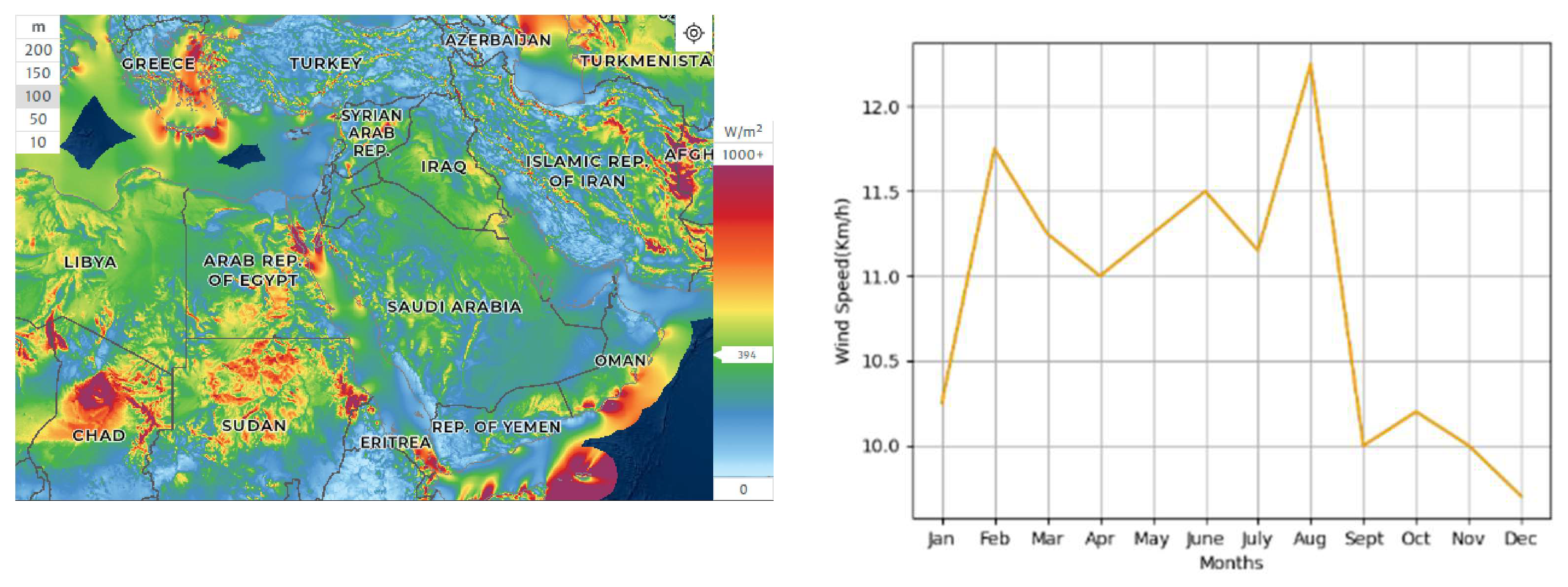
• The goal is to enhance the efficient operation of renewable energy systems, especially in the Middle East region.
• The target is to mitigate problems associated with decentralized energy sources (such as wind and solar) and to facilitate the efficient operation of an RE system in the Middle East region.
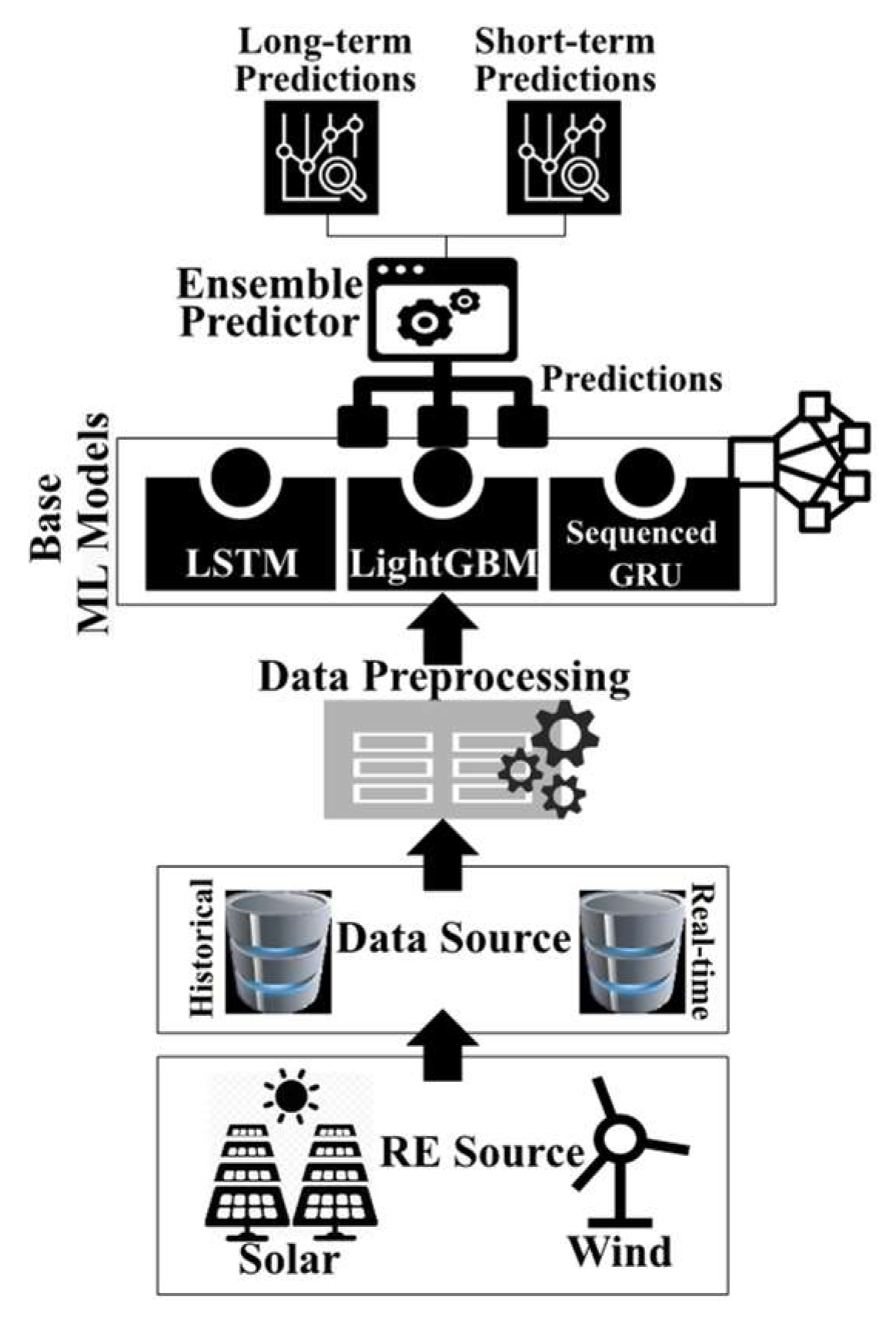
• The solution is to propose new forecasting approaches that use an ensemble mechanism.
• Making long-term and short-term predictions on RE generation in the Middle East region based on historical data.
• Further, the research contributions are highlighted as follows:
• This research introduces a novel approach using various ANN models to accurately forecast energy production from renewable sources like wind and solar.
• An advanced ensemble learning technique is incorporated, enhancing prediction accuracy beyond traditional models.
• The proposed methodology outperforms existing models in predicting both wind and solar power, showcasing superior metrics such as an optimal R² value of 0.9821.

The article is organized as follows: Section 2 presents relevant research, Section 3 outlines the issue statement, datasets, and ML approach using the suggested EL model, Section 4 presents the findings and effectiveness evaluation of the proposed EL model using experimental data, and Section 5 concludes the investigation.

2. Related Work

Accurate predictions are essential for various energy system functions to achieve both short-term and long-term goals. Figure 2 illustrates different forecasting methodologies, with machine learning techniques being widely used in various renewable energy applications. Recently, wind and solar power generation forecasting has improved significantly with the introduction of stochastic short-term prediction models.

Deterministic techniques are favored for their precise decision-making capabilities and the ability to select specific instances or measure the dispersion of the prospective estimation method. Juban et al. (2007) [17] proposed a unique non-parametric distributing strategy, known as “full predictive pattern”, which estimates core intensity using a blended intermittent continuous approach. Shu et al. (2015) [18] conducted research on predicting approaches for wind velocity and power, as well as solar radiation.

According to Foley et al. (2012) [19], wind power production from a single rotor can be predicted in advance ranging from 1 h to 12 days using a sequence-to-sequence neural network system. Olaofe et al. (2012) [20] employed various feed-forward neural network models to make multi-step predictions for longer-term periods, ranging from 30 to 360 min at 30 min intervals. Similarly, Cadenas-Barrera et al. (2013) [21] used a 2-layer feed-forward neural network method for renewable energy predictions.

López et al. (2018) [22] utilized principal component analysis to reduce the number of attributes used in LSTM-based estimates for numerical weather prediction. Xiong et al. (2021) [23] developed LSTM-based models for predicting renewable power. They integrated time-series attributes and observable traits to capture the best time-oriented physical characteristics. Liu et al. (2018) [24] used LSTM in a unique multiphase prediction approach for wind velocity, combining solitary spectral analysis, finite difference feature decomposition, LSTM, and ELM (extreme learning machine) models. Chen et al. (2018) [25] introduced a new LSTM architecture for estimating renewable power, utilizing the echo phase sector as connectivity hidden units.

In order to predict energy demand and interpret the statistical significance of available attributes, Sun et al. (2015) [26] employed a least-squares-SVM model optimized using the Bat refinement methodology. Bonanno et al. (2015) [27] utilized an RNN trained on wavelets for wind speed prediction, employing a dimension reduction method. Chang et al. (2016) [28] suggested a statistical approach using ARIMA to convert non-stationary wind records into stable trend lines. Brusca et al. (2017) [29] proposed a spiking driven NN approach for wind energy forecasting.

The study by Catalão et al. (2011) [30] introduced a unique 3-tiered feed-forward ANN approach optimized with the Levenberg-Marquardt method to predict RE in Portugal. Jursa & Rohrig (2008) [31] aimed to develop a novel procedure for short-term renewable energy estimation by integrating adaptive optimizer techniques. Particle-swarm optimization and dynamic optimization were evaluated, and ANN and a nearby search algorithm were utilized as prediction tools. A recent study by et al. (2022) [32] proposed an integrated approach using satellite data, radiative transfer modelling, and machine learning to predict solar irradiance over the Arabian Peninsula. Their methodology leveraged geosynchronous satellite data on cloud properties as input into a radiative transfer model for estimating surface solar irradiance.

Using ANN with optimization via particle swarms has increased the confidence interval to 9.6%. Combining the results from the closest neighbor lookup and NN models has reduced the confidence interval by around 10.75%. The review of RE forecasting research shows that diversification/heterogeneity is crucial in creating an effective prediction model. LSTM and standard ML models are used to implement heterogeneity and evaluate the outcomes. A two-step forecasting model is used to make more accurate predictions. The information about various studies on renewable energy forecasting using machine learning techniques is summarized in

Table 1. Summary of renewable energy prediction studies.

Study Reference	Location/Coordinates	Datasets Used	Methods/Techniques	Advantages
Juban et.al. (2007) [17]	Portugal	Not specified	Proposed unique non-parametric distributing strategy, “full predictive pattern”, using blended intermittent continuous approach	Can be used for various prediction types like periodic forecasts, parametric forecasts, spot estimates
Shu et al. (2015) [18]	Hong Kong	Wind velocity, power, solar radiation	Covariance, fuzzy analysis, convolutional neural networks, autoregressive additive neural networks, support vector machines, RBFNN, multi-stage ANN, non-linear multiple regression	Evaluated using RMSE and MAPE
Foley et al. (2012) [19]	Not specified	Wind power data	Sequence-to-sequence neural network	Can predict wind power 1 h to 12 days ahead
Olaofe et al. (2012) [20]	Not specified	Wind power data	Feed-forward neural networks	Multi-step predictions from 30 to 360 min
Cadenas-Barrera et al. (2013) [21]	Not specified	Renewable energy data	2-layer feed-forward neural network	Renewable energy prediction
López et al. (2018) [22]	Not specified	Numerical weather prediction data	LSTM, PCA, backpropagation neural networks, support vector machines	LSTM showed higher precision
Xiong et al. (2021) [23]	Not specified	Renewable power data	LSTM models with time series and observable features	Captures best time-oriented physical characteristics
Liu et al. (2018) [24]	Not specified	Wind velocity data	LSTM, spectral analysis, finite difference feature decomposition, ELM	Unique multiphase prediction approach
Chen et al. (2018) [25]	Not specified	Renewable power data	Novel LSTM architecture with echo state connectivity	Renewable power estimation
Sun et al. (2015) [26]	Not specified	Energy demand data, available attributes	Least squares SVM with bat optimization	Predict energy demand, interpret statistical significance of attributes
Bonanno et al. (2015) [27]	Not specified	Wind speed data	RNN trained on wavelets with dimension reduction	Wind speed prediction
Chang et al. (2016) [28]	Not specified	Wind data	ARIMA statistical approach	Converts non-stationary wind data to stable trends
Brusca et al. (2017) [29]	Not specified	Wind data	Spiking neural networks	Wind energy forecasting
Catalão et al. (2011) [30]	Portugal	Renewable energy data	3-tier feedforward ANN with Levenberg-Marquardt optimization	MAPE 7.26%, outperformed persistence and linear models
Jursa & Rohrig (2008) [31]	Not specified	Renewable energy data	ANN, particle swarm optimization, dynamic optimization	Explored variable selection and optimization for better forecasting
Al-Yahyai et al. (2010) [33]	Middle East	Historical wind speed data from weather stations across Middle East countries. Also used NWP model output data.	Reviewed the application of NWP models like WRF, MM5, and HRM for wind resource assessment across the Middle East. Evaluated model performance by comparing outputs to observational data.	Reviewed NWP models for wind energy estimation across the Middle East.

.

Furthermore, wind and solar energy systems face the following challenges:

• Issues with grid safety and power failures
• Issues with system reliability
• Dispatching and scheduler issues
• Essentiality of supplemental services
• Concerns regarding maintaining a stable electricity supply
• The challenge of administration and regulation
• The destruction of expensive electricity infrastructure
• Distressing financial conditions

Accurate prediction of wind and solar irradiance is crucial to overcome constraints that arise from integrating decentralized energy sources, especially renewables like wind and solar, into the energy grid. These sources have variable and intermittent characteristics that can impact their productivity. The study aims to develop methods for forecasting power generation using solar irradiance and wind energy.

3. Methodology

This section explores potential suggested concepts for enhancing the effectiveness of RE (solar and wind power) forecasting methods.

3.1. Problem Statement

According to the main objectives of this investigation, the issue of forecasting RE production (via wind and solar power) can be specified as follows. For an applicable time series of past records from datasets and real-time information, the issue of predicting energy output through solar and wind power can be described as,

$${\widehat{\mathbb{P}}}_s\left(t\right)=f\left[\rho (t-1)\cdots \rho (t-n)\right]$$

(1)

$${\widehat{\mathbb{P}}}_w\left(t\right)=f\left[ɸ(t-1)\cdots ɸ(t-n)\right]$$

(2)

where, ${\widehat{\mathbb{P}}}_s\left(t\right)$ and ${\widehat{\mathbb{P}}}_w\left(t\right)$ represents the prediction status of power generation via solar and wind sources at time t, respectively. ‘n’ denotes varying significant parameters, ${\mathbb{P}}_s\left(t\right)$ and ${\mathbb{P}}_w\left(t\right)$ indicate the actual energy produced via solar and wind sources at time t, respectively, and $\rho (t-n)$ signifies the potentiality of power produced in the past. Figure 3 illustrates the prediction model developed to analyze the forecast trends.

3.2. Dataset

The key element in RE forecasting is the collection and analysis of information. Preprocessing of the entire dataset is essential, involving tasks like normalization, removing irrelevant information, data segmentation, and studying relationships among different data attributes to gain insights. For this research, two datasets were used to train and evaluate the proposed model: [34,35]. Based on the references, some of the key features used to predict wind and solar energy production are:

For solar:

• Solar irradiance (W/m²)
• Air temperature (°C)
• Relative humidity (%)
• Atmospheric pressure (Pascals)
• Rainfall (mm)
• Location coordinates (latitude, longitude, elevation)

For wind:

• Wind speed (m/s)
• Wind direction (degrees)
• Air temperature (°C)
• Air pressure (Pascals)

The data for these parameters come from meteorological stations. The time granularity ranges from 10 min to hourly measurements. These weather and atmospheric data points serve as input features to machine learning models that are trained to predict the potential wind and solar energy generation. The models learn the relationships between the inputs and the actual renewable energy produced to make forecasts. Significant input variables of the datasets are listed in Figure 4.

Solar power is a promising renewable energy source, capable of harnessing solar radiation for thermal and electrical use [36]. It is environmentally friendly, producing zero greenhouse emissions compared to fossil fuels. However, estimating solar irradiance is complex due to various meteorological factors [37]. Machine learning techniques are often used for monthly, weekly, and hourly irradiance predictions due to inherent uncertainty [38].

Wind energy’s primary application is converting the kinetic energy of air into electricity onshore or offshore [39]. Wind power depends on solar irradiance, wind speed, and other conditions. Forecasting is essential due to wind power intermittency and uncertainty [40]. Wind power prediction can be categorized based on time-horizons [41], and techniques range from physical to statistical or machine learning approaches [42]. Accurate wind power prediction is challenging due to wind speed intermittency. Dynamic ANN-based techniques, considering multiple variables, are preferred for improved long/short-term forecasting accuracy) [43].

Normalizing the data, getting rid of any incomplete entries, and flagging any outliers are all part of the preprocessing phase. Data resizing is conducted at the first stage of normalization to transform the actual data descriptor from values ranging from [0, 1] to [1, 1] intervals. Scaling the information to an appropriate extent is essential for further processing since various configurations (like coefficients) make this assumption. The estimation for this normalization process is given in Equation (3):

$$D^s=\raisebox{1ex}{$\left[D-min\left(D\right)\right]$}\!\left/ \!\raisebox{-1ex}{$M\left(D\right)-m\left(D\right)$}\right.$$

(3)

The length of the data samples, represented by M(D) for the longest and m(D) for the shortest, can be irregular due to insufficient or incomplete training data caused by anomalous data collection techniques. For example, night-time solar radiation measurements provide no useful information for forecasting solar energy effectiveness. Therefore, it is necessary to remove anomalies from the data. Any subsamples can be evaluated using feature selection to eliminate inconsequential or inappropriate data points. Feature filtering narrows down a large set of potential features to a more manageable subset by removing redundant alternatives. With the reduced feature set, a model can be trained more efficiently, improve predictive performance, gain deeper data insights, and retain essential information. This study’s methodological framework addresses problems with the feature vector space. Even reliable datasets may have issues like redundant or repetitive features, noise, and missing data.

The methodological framework of this study addresses data irregularities in the feature space caused by insufficient or incomplete training datasets. To eliminate anomalies, a feature selection approach is employed, using the Relief algorithm proposed by Kira and Rendell (1992) [44]. This algorithm ranks and selects the most important features by considering their significance, relationships, and context. By choosing crucial characteristics through analytical techniques, the Relief algorithm creates a final training set with relevant attributes.

3.3. Primary Base Models

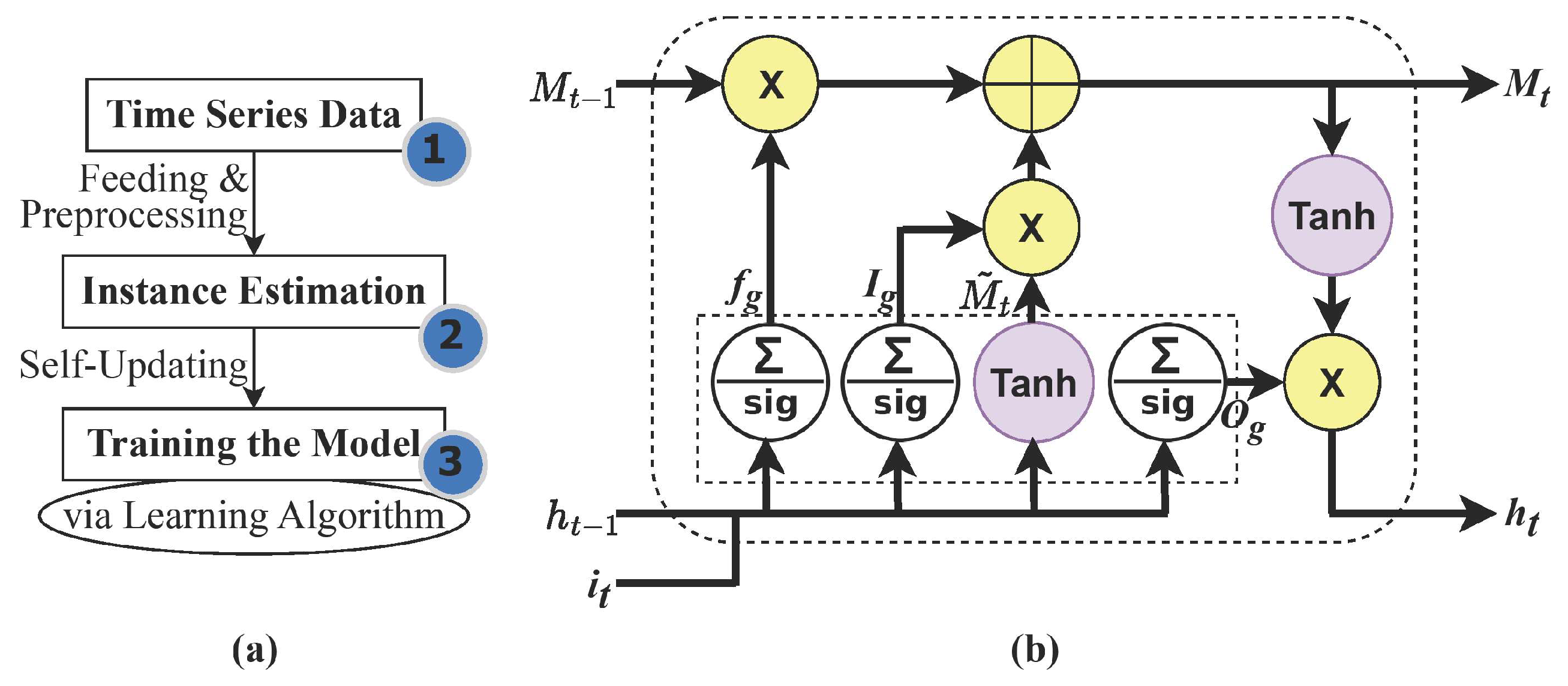
Effective modeling methodologies are essential for managing the operational aspects of RE in decentralized smart grids. Machine learning-based predictive models have proven to be valuable tools for RE generation forecasting. This study focuses on the preliminary prediction stage, utilizing major base models such as LSTM, LightGBM, and sequenced-GRU, to forecast energy production from solar and wind sources. In subsequent stages, an ensemble learning approach is employed. The suggested strategy for forecasting solar and wind power generation is summarized in Figure 5.

3.3.1. LSTM

The RNN provides the conceptual basis of the LSTM by Li et al. (2019) [45]. The ability to remember data that have been propagated through networks over a long duration is the most distinguishing feature and capability of the LSTM approach. A correlation of the previous knowledge will be produced as the forecast outcome. The LSTM paradigm utilizes 3 distinct gated operators [46,47]. They involve:

Forget Gate: signified as a decision-maker to preserve the data or not.

Input Gate: responsible for activating the fed input source from the preceding block.

Output Gate: a decision gate specifies the prediction estimate passed on to the next memory array. Deep neural networks often use this function because its output is constrained between zero and one. The corresponding formula is as follows:

$$Sig\left(x\right)=\raisebox{1ex}{$1$}\!\left/ \!\raisebox{-1ex}{$\left(1+e^{-x}\right)$}\right.$$

(4)

As a replacement for the older likelihood regression, whose outcome was restricted to the range from (−1) to (1), the tanh (hyperbolic tangent) operation was developed. This function’s trend line is symmetrical and imparts a non-linearity property to the network elements. The following is the formulation for the tanh activity mechanism:

$$\tanh \left(x\right)=\raisebox{1ex}{$\left[\left(e^x\right)-\left(e^{-x}\right)\right]$}\!\left/ \!\raisebox{-1ex}{$\left[\left(e^x\right)+\left(e^{-x}\right)\right]$}\right.$$

(5)

Figure 6a illustrates the three basic operational processes of the LSTM model: feeding and preprocessing of time-series data, and self-updating through continuous learning and training procedures. Figure 6b shows that the LSTM model requires two input patterns for training: the present time-series input, I_t and the earlier hidden state, h_t−1, and the cell provides the present output of h_t. M_t is the memory cell component and the important fact in the block is that it allows the information to travel along the entire chain with some minor linear interactions, i.e., no change in the cell state to hold the integrity of the data in the future [46]. The output h_t is calculated by the activation of cell state with the logical operation and nonlinear transformation of input. The equations from (6) to (9) that represent input–output association in the LSTM model are expressed as follows [48]:

$$f_g=\varsigma \left[\left(x_t·w_{fx}\right)+(h_{\left(t-1\right)}·w_{fh})+e_f\right]$$

(6)

$$I_g=\varsigma \left[\left(x_t·w_{Ix}\right)+(h_{\left(t-1\right)}·w_{Ih})+e_I\right]$$

(7)

$$M_g=tanh\left[\left(x_t·w_{Mx}\right)+(h_{\left(t-1\right)}·w_{Mh})+e_M\right]$$

(8)

$$O_g=\varsigma \left[\left(x_t·w_{Ox}\right)+(h_{\left(t-1\right)}·w_{Oh})+e_O\right]$$

(9)

where I_g, F_g, and O_g represent the input, forget, and output gates, respectively. The weighted vectors are indicated by w_Ix, w_fx, w_Mx, w_Ox, w_Ih, w_fh, w_Mh, and w_Oh, and the biases of each gate are denoted as e_f, e_I, e_M, and e_O. The homogeneity and conventional back-propagation mechanism are used to adjust and revisions to those parametric values as part of the typical NN learning routine. The message stream is regulated through a value ranging from zero to one the as output of the sigmoid process (ς). After the input state is amplified to produce the ${\widehat{M}}_t$ vector via the hyperbolic tangent (tanh), it is then appended to the previous state. Further, the information is passed to another layer of tanh. Finally, it is multiplied using the sigmoidal process to derive the output, h_t. The processes of I_g, F_g, and M_t−1 each contribute a significant role in the determination of the following and newer state parametric value, M_t. Following the acquisition of the new M_t, the resulting outcome, h_t, can be calculated via formulations as expressed in Equations (10) and (11):

$$M_t=\left[\left(f_g\times M_{t-1}\right)+\left(I_g\times {\widehat{M}}_t\right)\right]$$

(10)

$$h_t=\left[O_t\times tanh\left(M_t\right)\right]$$

(11)

From the above Equations (10) and (11), the product of the components is denoted by (×). The hidden layer’s fundamental goal is to train and refine the process of extracting useful data/facts while forgetting and eventually discarding irrelevant data. Sometimes, increasing hidden layers in LSTM may improve the model’s non-linear adaptation capabilities and its potential for training.

3.3.2. LightGBM

The fundamental principle of LightGBM is to progressively integrate L weaker trees (regression) into robust classification trees from Pan et al. (2020) [49]. A simple computation procedure is depicted in Equation (12):

$$O_f\left(y\right)={\sum }_{n=1}^N\left[{\mathbb{o}}_f\left(y\right)\right]$$

(12)

where 𝕠_f(y) represents the result of the n^th regression tree (weak), while O_f(y) reflects the ultimate outcome.

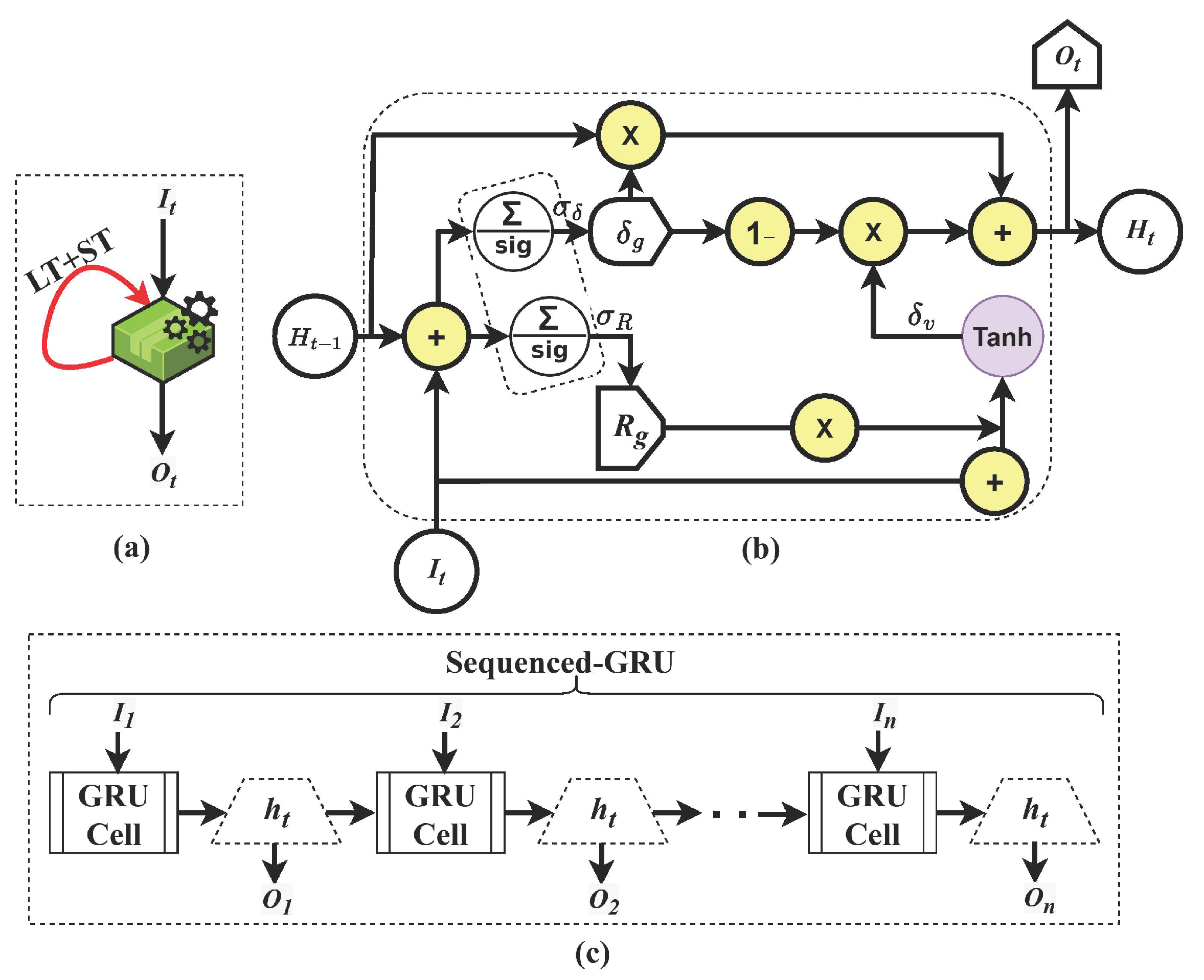
3.3.3. Sequenced-GRU

Sequential cells of the GRU perform calculations to generate the internal state (hidden state), allowing the GRU to retain relationships or memories for extended periods of time. Exactly one of a GRU’s hidden states is carried over from one sampling interval to the next. Figure 7a depicts the regulating processes through gates and operations performed through a hidden state and passing through input values to enable the internal state that contains both the short-term and long-term dependencies. Both the reset gate (R_g) and the update gate (δ_g) make up the whole of the sequential cells of GRU. In Figure 7b, the sequential processes are symbolized, where “×”, “−1”, and “+” signify the sequential operations, and σ_R, σ_δ symbols indicate the sigmoid features used in the update and reset gates, respectively. Figure 7c depicts the sequential process of multiple GRU cells with multiple hidden states, which expands on this model’s ability to handle multi-variate inputted data.

For each cycle, the result is calculated as a function of the vectors I_t of inputs and the resulting vector H_(t−1) preceding the result. The continuity equations from (13) to (16) explain the sequence of non-linear procedures that a feed undergoes to generate an appropriate outcome.

$$R\left(t\right)={\sigma }_g\left[\left(I_t·{\omega }_R\right)+\left({\eta }_R·H(t-1)\right)+\left(e_R\right)\right]$$

(13)

$$\delta \left(t\right)={\delta }_g\left[\left(I_t·{\omega }_{\delta }\right)+\left({\eta }_{\delta }·H(t-1)\right)+\left(e_{\delta }\right)\right]$$

(14)

$$H\left(t\right)=\left[\left(\delta \left(t\right)·H\left(t\right)\right)+\left(1-\delta \left(t\right)\right)·H(t-1)\right]$$

(15)

$$H\left(t\right)=Tanh\left[\left(I_t·{\omega }_H\right)+\left({\eta }_H·H(t-1)\right)+\left(e_H\right)\right]$$

(16)

where R(t) represents the reset vector; δ_v denotes update vector; ω, η, depict the vectors of configurable matrices; σ signifies the sigmoid transfer component; and Tanh indicates the highly non-linear transfer functions (hyperbolic tangent).

3.3.4. Ensemble Learning (EL) Method

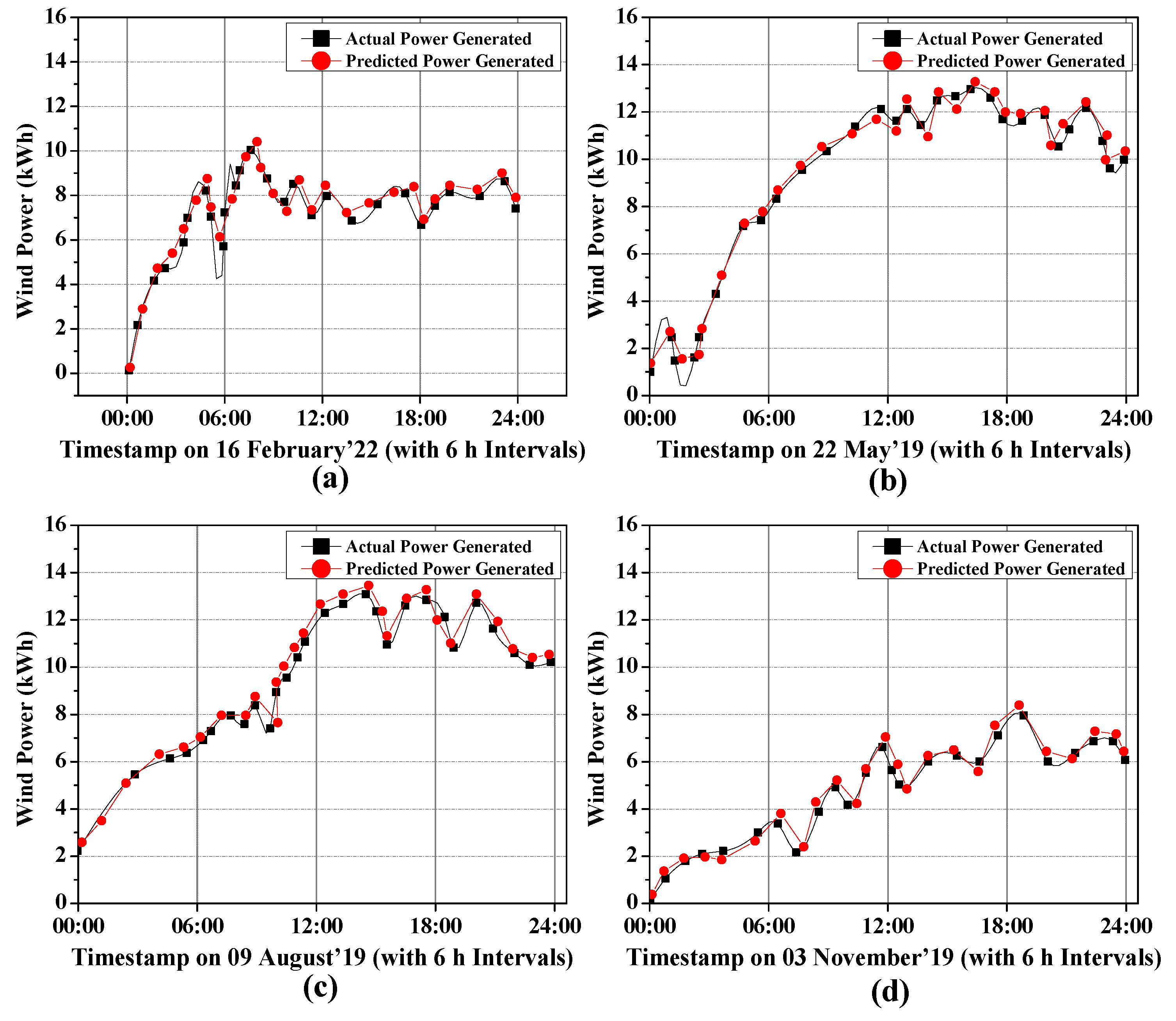
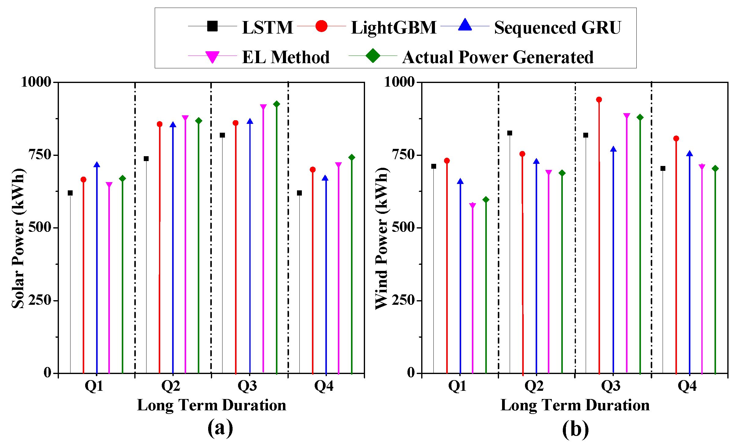
Using multiple forecasting models together to enhance prediction accuracy is a promising subject of research. We propose an EL-based hybrid model that combines ML and other base predictors for predicting solar and wind power output. Various ensemble strategies are employed to obtain the final power generation forecast by combining projections from different modeling techniques. This approach can improve the system’s performance by introducing diversity among the merged models. Ensemble techniques are classified as structural and data-based, as shown in Figure 8.

In this systematic research, we assess the proposed EL method using two alternative ensemble approaches. The following are the considered ensemble techniques:

Simple Averaging (SA): The overall solar power prediction is derived using the most common and intuitive method called the “simple averaging method”, which is an arithmetically aggregating of the individual estimates produced by several base models. The computation role implied in the prediction of solar power generation via SA is depicted in Equation (17):

$$F_{⟨S|W⟩}=\raisebox{1ex}{$\left[{\widehat{F}}_{⟨S|W⟩}^{LightGBM}+{\widehat{F}}_{⟨S|W⟩}^{LSTM}+{\widehat{F}}_{⟨S|W⟩}^{Sequenced\_GRU}\right]$}\!\left/ \!\raisebox{-1ex}{$k$}\right.$$

(17)

In Equation (17), $F_{⟨S|W⟩}$ represents the overall prediction of solar and wind power; k denotes the count of considered base predictors (k = 3); and $\widehat{F}$ signifies the prediction outcome of individual base predictors.

Stacking Ensemble (SE): SE is an EL approach that utilizes meta-learning to integrate multiple individual ML algorithms. Each meta-learner technique is trained using the results of all base predictors and a common dataset. The key findings from the underlying models are used to enhance the meta-learner through sufficient training. This procedure enables the use of a wide variety of learners, each with its unique set of assumptions and procedures. Two crucial distinctions between stacking and other methods (boosting or bagging) are that SE considers non-homogeneous weak predictors (ML algorithms) for learning and uses a meta-learner to integrate the base predictors. The strength of stacking lies in its ability to combine several high-performing methods for a specific prediction task, resulting in superior estimates compared to other predictive techniques.

4. Model Evaluation

Ultimately, this study’s goal is to test and validate the efficacy of the suggested approach by conducting many empirical runs to predict a day-ahead RE (wind and solar) power delivery. Python v3.7 (via Keras Application Programming Interfaces) (Team, n.d.) [50] and the TensorFlow platform v2 (Install TensorFlow 2, n.d.) [51] were used to create the suggested models. The predictor algorithms were adapted with the use of the effective RMSProp optimization procedure [52]. The settings were examined in the context of the analytical method as described in the following: weight updating in 15 batches, with 500 epochs of execution. In addition,

Table 2. Essential hyperparameters.

Parameters	Range
	LSTM	LightGBM	Sequenced GRU
Hidden Layer/State Count	2	2	1/It
Sequence Length	15	11	11
Batch Size	15	13	13
Activation Function	2	1	1
Max. Tree Depth	-	10	-
Subsamples	-	0.5	-
Optimizer	RMSProp
Learning Rate	0.0001
Training Set Ratio	80
Testing Set Ratio	20
Epoch Count	500

represents the essential hyperparameters of each predictor algorithm.

The training process involves evaluating the expected outcome deviation and tuning the parametric weight values in each stage until the deviation is small enough. Mean-bias-error (MBE), MAPE, RMSE, and R² (coefficient of determination) are some of the major unpredictability measures employed to determine the efficacy of the modeling approaches which were used in establishing the optimal prediction of RE generation and validating error. The higher the accuracy of a prediction, the maximum lesser observable values of RMSE, MAPE, and MAE will be considered optimal for any forecasting model.

The RMSE is characterized as the difference (bias) between the assessed value (${\mathbf{ʠ}}_{\mathit{v}}$) and the predicted values (${\mathbf{ϻ}}_{\mathit{v}}$) divided by the overall observation count (X). The computation part of RMSE is expressed in Equation (18):

$$RMSE=\sqrt{\raisebox{1ex}{$1$}\!\left/ \!\raisebox{-1ex}{$X$}\right.}·\sqrt{{\sum }_{v=1}^X{\left[\left({ʠ}_v\right)-\left({ϻ}_v\right)\right]}^2}$$

(18)

MAPE, as well as MAE, also represent measurements of forecasting efficiency, wherein MAE is referred to as an estimation of the mean bias between the values obtained and the actual measurements. MAPE expresses the proportion of forecasting precision proposed by de Myttenaere et al. (2016) [53]. The computing formulation of both MAPE and MAE is expressed in Equations (19) and (20), respectively:

$$MAPE=\raisebox{1ex}{$1$}\!\left/ \!\raisebox{-1ex}{$X$}\right.·{\sum }_{v=1}^X\left(\raisebox{1ex}{$\left|\left({ʠ}_v\right)-\left({ϻ}_v\right)\right|$}\!\left/ \!\raisebox{-1ex}{${ʠ}_v$}\right.\right)\times 100$$

(19)

$$MAE=\raisebox{1ex}{$1$}\!\left/ \!\raisebox{-1ex}{$X$}\right.·{\sum }_{v=1}^X\left|\left({ʠ}_v\right)-\left({ϻ}_v\right)\right|$$

(20)

R², the predictability coefficient, states the unpredictability assessment with a quantitative measure (limited from 0 to 1). If the observable values approach one or nearer, it tends to show that the predicted values were substantially matched to the experimental measurements. Equation (21) exhibits the formulation R² as follows:

$$R^2=1-\left[\frac{{\sum }_{v=1}^X{\left[\left({ʠ}_v\right)-\left({ϻ}_v\right)\right]}^2}{{\sum }_{v=1}^X{\left[\left({\overline{ʠ}}_v\right)-\left({\overline{ϻ}}_v\right)\right]}^2}\right]$$

(21)

The time scale for short-term prediction ranges from one to six hours ahead. Moreover, it is a significant element in load management, scheduling, and congestion control processes. The accessible datasets have been divided into four quarters, with an 80:20 (training and testing) split between short- and long-term projections, as shown in the

Table 3. Testing and training data segregation for short- and long-term predictions.

Quarters	Long Term	Short Term (6 h Interval)
Q1	January–22 March ⸸	Wednesday–February ’22 ⸸
Q2	April–19 June ⁕	Wednesday–May ’19 ⁕
Q3	July–19 September ⁕	Friday–August ’19 ⁕
Q4	October–19 December ⁕	Sunday–November ’19 ⁕

^⁕ [34].^⸸ [35].

.

With reliable short-term forecasting of wind power generation, energy distribution operators may predict and prepare for wind power variations, reducing the negative effects of intermittent wind renewables. The speed of the wind is the primary determinant of the proportion of power a windmill rotor can generate. Whenever these rotors spin at a faster rate under stronger winds, the amount of energy generated will be higher. Additionally, wind speed dramatically impacts the effectiveness at which a turbine blade transforms renewable power into electricity. Figure 9 represents the average annual wind speed map across the Middle East, along with a monthly average wind speed graph. From February through August, the wind speed graph shows relatively high values, which might result in the turbine producing more electricity than usual.

The above-mentioned recommended approach was used to carry out the experimental studies on the chosen dataset. We use the sample sets and the resulting base models to examine the proposed forecasting approach further to conduct training. The models increased their forecasting abilities by learning the patterns and trends of energy generation. Figure 10a–d display empirical performance details that suggest the prediction models deliver more consistent and accurate results while equated to other base models’ forecasting outcomes and illustrate the short-term electricity production on four distinct timeframes (4 days with 6 h intervals). Here, we use the past records of generated wind power to construct a timestamp at regular intervals (every 6 h). A 6 h ahead forecast of wind and solar generation can assist in power system operations like scheduling, dispatch, and trading. This procedure heads off reliability issues from renewable variability.

In most cases, the suggested model’s precision will decrease if such training is insufficient or not validated (preprocessed). The training was halted whenever the prediction error remained unchanged after 150 epochs to prevent over-fitting. The recorded wind speed is around 11.24–12.25 Km/h for the period May to August in the concerned region, so it stands to reason that wind power production would be highest during these times. The findings in Figure 10 confirm what was already shown in Figure 9, that wind power production is significantly reliant on wind speed and other meteorological parameters. After four days of observation, it is noticeable that the measurement predicted one day (24 h) in advance is more appropriate. Following the initial six hours, the erroneous rate settled into a narrow range of 10–20% during the four days. Over all projected days, the forecasting system showed reduced error relative to the proposed model.

In regions featuring substantial solar coverage, variations in renewable power production happen, caused by short-term phenomena (such as passing skies) that could have significant effects. This is especially the case with photovoltaic-based solar farms, where modules/panels are clustered strategically. This is why much work has gone into predicting solar power production using different techniques. Figure 11 visually represents how well the EL model can forecast short-term solar power production. Furthermore, it has been shown that the confidence interval is much more prominent when considering the unpredictability of solar energy. Figure 12a–d illustrate measurements and evaluations that confirm the EL model’s excellence and progress in terms of their respective forecasting uses.

Additionally, we show that the EL model outperforms the competition in terms of both moment-in-time forecasting and interval prediction. Unfortunately, there are insufficient essential data to determine whether solar power follows a monthly or yearly pattern. Therefore, in order to refine the model’s architecture, a mix of factors such as the date, time of day, and precipitation is provided as input to train the model. It seems logical that the peak output of power would occur between the months of May and October when the region’s average temperature is between 40° to 42° Celsius. Apart from the last six hours, the erroneous prediction rate is found to be below 10%. However, due to the irradiance uncertainties (below the horizon), the erroneous range is slightly higher than other interval periods.

Figure 13 shows the forecasting results of the wind and solar power generation compared with the real data over 24-hr ahead time horizon. Results of all four models are analyzed in contrast to the actual results. The outcome of the proposed model appropriately predicts the power generation which matches with the results of the actual outcome. Out of other three models, the sequenced-GRU performs better than the LightGBM and standard LSTM. The sequenced-GRU has some commonalities with those characteristics, which has features that are comparable to those of the LSTM NN but has a lower learning rate in order to optimize the training period. LSTM comprises an input, a forget, and an output gate, but in sequenced-GRU, both the input and forget gates are combined to speed up the training. The proposed EL model outperforms LSTM, LightGBM, and sequenced-GRU due to its operational excellence in both convergence and parameterization adjustments. However, the LightGBM model follows the leaf-based segregation in the tree, which might result in overfitting since the models tend to generate more complicated trees. Because of this, LightGBM is sensitive to problems with oversampling and may quickly overfit sparse samples as well. Figure 13a shows the outcome of all four models’ 24-h ahead wind power forecasts. When analyzed with actual output, the proposed EL model registers the most minor error margin ratio of 2.86%, whereas LSTM, LightGBM, and sequenced-GRU attain values of 3.24%, 4.12%, and 3.17%, respectively. However, wind power generation is highly influenced by nature and seasons, with few operational factors (radius of blade, air density, wind velocity), that directly impact production and forecasting potential.

Similarly, Figure 13b depicts the graphical comparisons of all four models’ 24-h ahead predictions of solar power generation with actual generative outcomes. The EL model records a minimized error margin of 1.92%, whereas LSTM, LightGBM, and sequenced-GRU attain values of 3.67%, 3.52%, and 2.28%, respectively. Concerns about solar power production are primarily attributable to the ambient weather parameters and their accompanying intricacy and seasonality. However, due to the uncertainty of irradiance, solar power forecasting remains a challenging issue despite these advancements.

Effective solar and wind electricity generation prediction relying on precise weather forecasts provides considerable advantages to grid management over longer durations (e.g., months or seasonal periods), particularly when preparing for severe weather occurrences. However, when employing the same prediction model, the predictions’ precision drops as the estimated time horizon becomes longer. Therefore, ensuring a satisfactory degree of prediction accuracy necessitates the determination of a sufficient temporal horizon when building prediction models. Figure 14a exhibits the long-term power generation predictions of all considered models for both solar and wind. It signifies that the forecasting of the EL model in all four quarters appropriately matches the actual outcome. The error margin ratio of LSTM, LightGBM, sequenced-GRU, and EL models in all quarters for long-term wind power prediction is 4.23%, 3.15%, 2.89%, and 1.23%, respectively. Similarly, Figure 14b shows the error margin ratio of long-term solar predictions in all four quarters as 5.56%, 3.57%, 2.72%, and 1.73%, respectively.

The RMSE, MAE, and MAPE losses were used to assess the approaches’ effectiveness. Forecasting accuracy on a set of training data is evaluated across four models. Their relative scores are displayed in

Table 4. Evaluation of short- and long-term forecasting using different performance indices.

Methods	Short Term			Long Term
	MAE	RMSE	MAPE	MAE	RMSE	MAPE
LSTM	1.345	2.324	3.411	3.123	4.576	3.421
LightGBM	2.321	3.215	2.187	3.578	3.123	2.452
Sequenced GRU	0.971	1.546	1.089	2.107	1.792	1.834
EL Method	0.782	0.833	0.702	1.081	0.921	1.055

using measures such as mean absolute error; root mean squared error, mean absolute percent error, and the correlation coefficient (R²). In procedures, the lowest error margin represents the optimal result. When calculating the MAE, the total of the absolute variations between the observed and projected values is used. The MAPE measures precision as the dissimilarity between the observed and expected outcomes. As a practical matter, it may be generally said that the smaller the measurement of the RMSE, the superior the estimate is deemed to be. The produced model’s applicability is shown by the number of errors during the training phase, whereas the number of errors during the testing dataset demonstrates the generalization skills of a given approach. With an ideal learning rate and enhanced processing of larger values of weather conditions (like wind velocity) and uncertain irradiance, the EL model seems more effective at short-term and long-term power prediction of wind and solar than previous models. The presented indicators make it evident that the conventional LSTM approach has the worst results and the worst predicting error among the five ML methods.

For the four models, the R² scores range from 0.9215 to 0.9812. The EL model has the greatest R-value, whereas the other algorithms shown in Figure 15 have lower R² values. Sequenced-GRU is preferable for predicting solar irradiance since its R-value is higher (0.9644) and the gap between the testing and training R-values is smaller. LSTM layers are extremely memory-intensive, to the point that they are typically limited in their ability to use the platform’s processing resources. The shortcomings of LightGBM involve no premature halting, poor precision, and shorter training.

5. Conclusions

Predicting RE sources, such as solar and wind, is getting more important as their use spreads throughout the globe. This is certainly relevant when considering a sophisticated utility grid and incorporating these energies into the primary electrical system. The solution is to propose new forecasting approaches that use an ensemble mechanism to make long-term and short-term predictions on RE generation in the Middle East based on historical data. With the goal of maximizing precision (accuracy) and minimizing error, ensemble-based hybrid forecasting methods have been proposed. A unique and analytical EL-based model is the intended outcome of this proposed research. The reliability and efficiency of RE hourly (24 h ahead of time) prediction models have greatly improved. The EL methodology is more accurate than LSTM, LightGBM, and sequenced-GRU for predicting wind power and solar power. It also registered an optimal R² value of 0.9821. An ensemble of ineffective learners is employed to boost the ML model’s accuracy via the EL technique. When their findings are integrated, superior models are produced. In addition, LightGBM is not resilient and is technically unfeasible; thus, even minor modifications to the training sample might result in drastically altered tree topologies and, ultimately, unexpected forecasts for the equivalent testing set. Our proposed method has been shown to be reasonably precise at calculating the likelihood of wind and solar power that may be generated on a given day as well as extended terms corresponding to the fed parameters (wind speed, irradiance, and other weather parameters), which is incredibly useful for the reasons already stated.

Future Work

By exploring more ML approaches, improving such algorithms for real-time predictions, and making different forecast intervals, the machine learning service described in the article can be extended to other domains such as fraud detection, recommendation systems, and predictive maintenance, which suggests that there may be potential for future research in these areas [54]. Transformer-based models [55], deep learning methodologies, and combining different RE into speed estimates are all things that could be studied further in the future.

References

1. Renewable Global Status Report REN21. Available online: https://www.ren21.net/reports/global-status-report/ (accessed on 13 June 2019).
2. Han, J.; Choi, C.; Park, W.; Lee, I.; Kim, S. Smart home energy management system including renewable energy based on ZigBee and PLC. IEEE Trans. Consum. Electron. 2014, 60, 198–202. [Google Scholar] [CrossRef]
3. Kazmierkowski, M.P.; Jasinski, M.; Wrona, G. DSP-Based Control of Grid-Connected Power Converters Operating Under Grid Distortions. IEEE Trans. Ind. Inform. 2011, 7, 204–211. [Google Scholar] [CrossRef]
4. Kumar, A.; Kumar, K.; Kaushik, N.; Sharma, S.; Mishra, S. Renewable energy in India: Current status and future potentials. Renew. Sustain. Energy Rev. 2010, 14, 2434–2442. [Google Scholar] [CrossRef]
5. Baseer, M.A.; Praveen, R.P.; Zubair, M.; Khalil, A.G.A.; Saduni, I.A. Performance and Optimization of Commercial Solar PV and PTC Plants. Int. J. Recent Technol. Eng. 2020, 8, 1703–1714. [Google Scholar] [CrossRef]
6. Baseer, M.A.; Almunif, A.; Alsaduni, I.; Zubair, M.; Tazeen, N. An adaptive power point tracker in wind photovoltaic system using an optimized deep learning framework. Energy Sources Part A: Recovery Util. Environ. Eff. 2022, 44, 4846–4861. [Google Scholar] [CrossRef]
7. BP. Statistical Review of World Energy. BP Global. 2021. Available online: https://www.bp.com/en/global/corporate/energy-economics/statistical-review-of-world-energy.html (accessed on 26 June 2023).
8. Baseer, M.A.; Alsaduni, I.; Zubair, M. Novel hybrid optimization maximum power point tracking and normalized intelligent control techniques for smart grid linked solar photovoltaic system. Energy Technol. 2021, 9, 2000980. [Google Scholar] [CrossRef]
9. Markovics, D.; Mayer, M.J. Comparison of machine learning methods for photovoltaic power forecasting based on numerical weather prediction. Renew. Sustain. Energy Rev. 2022, 161, 112364. [Google Scholar] [CrossRef]
10. Gao, H.; Qiu, S.; Fang, J.; Ma, N.; Wang, J.; Cheng, K.; Wang, H.; Zhu, Y.; Hu, D.; Liu, H.; et al. Short-Term Prediction of PV Power Based on Combined Modal Decomposition and NARX-LSTM-LightGBM. Sustainability 2023, 15, 8266. [Google Scholar] [CrossRef]
11. Ritchie, H.; Roser, M.; Rosado, P. Energy. 2022. Available online: https://ourworldindata.org/energy (accessed on 1 January 2022).
12. Badal, F.R.; Das, P.; Sarker, S.K.; Das, S.K. A survey on control issues in renewable energy integration and microgrid. Prot. Control. Mod. Power Syst. 2019, 4, 8. [Google Scholar] [CrossRef]
13. Advanced Energy Economy Institute. Integrating Renewable Energy into the Electricity Grid. Available online: https://info.aee.net/hubfs/EPA/AEEI-Renewables-Grid-Integration-Case-Studies.pdf (accessed on 25 August 2023).
14. Trends 2018 in Photovoltaic Applications Survey Report of Selected IEA Countries Between. 1992. Available online: https://iea-pvps.org/wp-content/uploads/2020/01/2018_iea-pvps_report_2018.pdf (accessed on 1 January 2018).
15. Tang, N.; Mao, S.; Wang, Y.; Nelms, R.M. Solar Power Generation Forecasting With a LASSO-Based Approach. IEEE Internet Things J. 2018, 5, 1090–1099. [Google Scholar] [CrossRef]
16. Wang, Y.; Liao, W.; Chang, Y. Gated Recurrent Unit Network-Based Short-Term Photovoltaic Forecasting. Energies 2018, 11, 2163. [Google Scholar] [CrossRef]
17. Juban, J.; Siebert, N.; Kariniotakis, G.N. Probabilistic Short-term Wind Power Forecasting for the Optimal Management of Wind Generation. In Proceedings of the 2007 IEEE Lausanne Power Tech, Lausanne, Switzerland, 1–5 July 2007. [Google Scholar] [CrossRef]
18. Shu, Z.R.; Li, Q.S.; Chan, P.W. Investigation of offshore wind energy potential in Hong Kong based on Weibull distribution function. Appl. Energy 2015, 156, 362–373. [Google Scholar] [CrossRef]
19. Foley, A.M.; Leahy, P.G.; Marvuglia, A.; McKeogh, E.J. Current methods and advances in forecasting of wind power generation. Renew. Energy 2012, 37, 1–8. [Google Scholar] [CrossRef]
20. Olaofe, Z.O.; Folly, K.A. Wind power estimation using recurrent neural network technique. In Proceedings of the IEEE Power and Energy Society Conference and Exposition in Africa: Intelligent Grid Integration of Renewable Energy Resources (PowerAfrica), Johannesburg, South Africa, 9–13 July 2012. [Google Scholar] [CrossRef]
21. Cardenas-Barrera, J.L.; Meng, J.; Castillo-Guerra, E.; Chang, L. A Neural Network Approach to Multi-step-ahead, Short-Term Wind Speed Forecasting. In Proceedings of the 2013 12th International Conference on Machine Learning and Applications, Miami, FL, USA, 4–7 December 2013. [Google Scholar] [CrossRef]
22. López, E.; Valle, C.; Allende, H.; Gil, E.; Madsen, H. Wind Power Forecasting Based on Echo State Networks and Long Short-Term Memory. Energies 2018, 11, 526. [Google Scholar] [CrossRef]
23. Xiong, B.; Meng, X.; Wang, R.; Wang, X.; Wang, Z. Combined Model for Short-term Wind Power Prediction Based on Deep Neural Network and Long Short-Term Memory. J. Phys. Conf. Ser. 2021, 1757, 012095. [Google Scholar] [CrossRef]
24. Liu, H.; Mi, X.; Li, Y. Smart multi-step deep learning model for wind speed forecasting based on variational mode decomposition, singular spectrum analysis, LSTM network and ELM. Energy Convers. Manag. 2018, 159, 54–64. [Google Scholar] [CrossRef]
25. Chen, J.; Zeng, G.-Q.; Zhou, W.; Du, W.; Lu, K.-D. Wind speed forecasting using nonlinear-learning ensemble of deep learning time series prediction and extremal optimization. Energy Convers. Manag. 2018, 165, 681–695. [Google Scholar] [CrossRef]
26. Sun, W.; Liu, M.; Liang, Y. Wind Speed Forecasting Based on FEEMD and LSSVM Optimized by the Bat Algorithm. Energies 2015, 8, 6585–6607. [Google Scholar] [CrossRef]
27. Bonanno, F.; Capizzi, G.; Sciuto, G.L.; Napoli, C. Wavelet recurrent neural network with semi-parametric input data preprocessing for micro-wind power forecasting in integrated generation Systems. In Proceedings of the 2015 International Conference on Clean Electrical Power (ICCEP), Taormina, Italy, 16–18 June 2015. [Google Scholar] [CrossRef]
28. Chang, G.W.; Lu, H.J.; Hsu, L.Y.; Chen, Y.Y. A hybrid model for forecasting wind speed and wind power generation. In Proceedings of the 2016 IEEE Power and Energy Society General Meeting (PESGM), Boston, MA, USA, 17–21 July 2016. [Google Scholar] [CrossRef]
29. Brusca, S.; Capizzi, G.; Lo Sciuto, G.; Susi, G. A new design methodology to predict wind farm energy production by means of a spiking neural network–based system. Int. J. Numer. Model. Electron. Netw. Devices Fields 2017, 32, e2267. [Google Scholar] [CrossRef]
30. Catalão, J.P.S.; Pousinho, H.M.I.; Mendes, V.M.F. Short-term wind power forecasting in Portugal by neural networks and wavelet transform. Renew. Energy 2011, 36, 1245–1251. [Google Scholar] [CrossRef]
31. Jursa, R.; Rohrig, K. Short-term wind power forecasting using evolutionary algorithms for the automated specification of artificial intelligence models. Int. J. Forecast. 2008, 24, 694–709. [Google Scholar] [CrossRef]
32. Alwadei, S.; Farahat, A.; Ahmed, M.; Kambezidis, H.D. Prediction of Solar Irradiance over the Arabian Peninsula: Satellite Data, Radiative Transfer Model, and Machine Learning Integration Approach. Appl. Sci. 2022, 12, 717. [Google Scholar] [CrossRef]
33. Al-Yahyai, S.; Charabi, Y.; Gastli, A. Review of the use of numerical weather prediction (NWP) models for wind energy assessment. Renew. Sustain. Energy Rev. 2010, 14, 3192–3198. [Google Scholar] [CrossRef]
34. IEA. Energy Production in the Middle East, 2019—Charts—Data & Statistics. 2019. Available online: https://www.iea.org/data-and-statistics/charts/energy-production-in-the-middle-east-2019 (accessed on 1 January 2019).
35. Wind & Solar Energy Data. 2022. Available online: https://datasource.kapsarc.org/explore/dataset/wind-solar-energy-data (accessed on 24 August 2022).
36. Arevalo, J.C.; Santos, F.; Rivera, S. Uncertainty cost functions for solar photovoltaic generation, wind energy generation, and plug-in electric vehicles: Mathematical expected value and verification by Monte Carlo simulation. Int. J. Power Energy Convers. 2019, 10, 171. [Google Scholar] [CrossRef]
37. Hejazi, M.-A.A.; Bamaga, O.A.; Al-Beirutty, M.H.; Gzara, L.; Abulkhair, H. Effect of intermittent operation on performance of a solar-powered membrane distillation system. Sep. Purif. Technol. 2019, 220, 300–308. [Google Scholar] [CrossRef]
38. Rocha, P.A.C.; Fernandes, J.L.; Modolo, A.B.; Lima, R.J.P.; da Silva, M.E.V.; Bezerra, C.A.D. Estimation of daily, weekly and monthly global solar radiation using ANNs and a long data set: A case study of Fortaleza, in Brazilian Northeast region. Int. J. Energy Environ. Eng. 2019, 10, 319–334. [Google Scholar] [CrossRef]
39. Shoaib, M.; Siddiqui, I.; Rehman, S.; Khan, S.; Alhems, L.M. Assessment of wind energy potential using wind energy conversion system. J. Clean. Prod. 2019, 216, 346–360. [Google Scholar] [CrossRef]
40. Imtiaz, S.; Altaf, M.W.; Riaz, A.; Naz, M.N.; Bhatti, M.K.; Hassan, R.G. Intermittent Wind Energy Assisted Micro-Grid Stability Enhancement Using Security Index Currents. In Proceedings of the 2019 15th International Conference on Emerging Technologies (ICET), Peshawar, Pakistan, 2–3 December 2019. [Google Scholar] [CrossRef]
41. Soman, S.S.; Zareipour, H.; Malik, O.; Mandal, P. A Review of Wind Power and Wind Speed Forecasting Methods with Different Time Horizons. In Proceedings of the 2010 North American Power Symposium, Arlington, TX, USA, 26–28 September 2010. [Google Scholar] [CrossRef]
42. More, A.; Deo, M.C. Forecasting wind with neural networks. Mar. Struct. 2003, 16, 35–49. [Google Scholar] [CrossRef]
43. Liu, H.; Chen, C.; Lv, X.; Wu, X.; Liu, M. Deterministic wind energy forecasting: A review of intelligent predictors and auxiliary methods. Energy Convers. Manag. 2019, 195, 328–345. [Google Scholar] [CrossRef]
44. Kira, K.; Rendell, L.A. A Practical Approach to Feature Selection. In Machine Learning Proceedings; Elsevier: Amsterdam, The Netherlands, 1992; pp. 249–256. [Google Scholar] [CrossRef]
45. Li, G.; Wang, H.; Zhang, S.; Xin, J.; Liu, H. Recurrent Neural Networks Based Photovoltaic Power Forecasting Approach. Energies 2019, 12, 2538. [Google Scholar] [CrossRef]
46. Olah, C. Understanding LSTM Networks—Colah’s Blog. Available online: https://colah.github.io/posts/2015-08-Understanding-LSTMs/ (accessed on 27 August 2015).
47. Dong, D.; Sheng, Z.; Yang, T. Wind power prediction based on recurrent neural network with long short-term memory units. In Proceedings of the 2018 International Conference on Renewable Energy and Power Engineering (REPE), Toronto, ON, Canada, 24–26 November 2018; pp. 34–38. [Google Scholar]
48. Jia, Y.; Wu, Z.; Xu, Y.; Ke, D.; Su, K. Long Short-Term Memory Projection Recurrent Neural Network Architectures for Piano’s Continuous Note Recognition. J. Robot. 2017, 2017, 2061827. [Google Scholar] [CrossRef]
49. Pan, Z.; Fang, S.; Wang, H. LightGBM Technique and Differential Evolution Algorithm-Based Multi-Objective Optimization Design of DS-APMM. IEEE Trans. Energy Convers. 2021, 36, 441–455. [Google Scholar] [CrossRef]
50. Available online: https://pypi.org/project/Keras-Applications/ (accessed on 30 May 2019).
51. Available online: https://www.tensorflow.org/install (accessed on 24 March 2023).
52. Zhang, A.; Lipton, Z.C.; Li, M.; Smola, A.J. Dive into Deep Learning. Available online: https://d2l.ai/chapter_optimization/rmsprop.html (accessed on 9 September 2022).
53. de Myttenaere, A.; Golden, B.; Le Grand, B.; Rossi, F. Mean Absolute Percentage Error for regression models. Neurocomputing 2016, 192, 38–48. [Google Scholar] [CrossRef]
54. Jain, M. Machine Learning Service for Real-Time Prediction. Towards Data Science. Available online: https://towardsdatascience.com/machine-learning-service-for-real-time-prediction-9f18d585a5e0 (accessed on 26 April 2021).
55. Lin, T.; Wang, Y.; Liu, X.; Qiu, X. A survey of transformers. J. Artif. Intell. Res. 2022, 3, 111–132. [Google Scholar] [CrossRef]
Figure 1. Renewable energy production in the Middle East [11].
Energies 16 06414 g001
Figure 2. Various types of forecasting techniques.
Energies 16 06414 g002
Figure 3. Prediction model.
Energies 16 06414 g003
Figure 4. Input variables to train the models.
Energies 16 06414 g004
Figure 5. Overview of proposed model.
Energies 16 06414 g005
Figure 6. (a) Procedure of LSTM, (b) generalized structure of LSTM.
Energies 16 06414 g006
Figure 7. (a) Generalized process of GRU, (b) GRU cell structure, and (c) sequenced process of GRU model.
Energies 16 06414 g007
Figure 8. Diversification of the EL approach.
Energies 16 06414 g008
Figure 9. Average wind speed (annual) in the Middle East [34,35].
Energies 16 06414 g009
Figure 10. Prediction accuracy estimation of short-term wind energy generation via EL model.
Energies 16 06414 g010
Figure 11. Annual average sun irradiance and power production in the Middle East.
Energies 16 06414 g011
Figure 12. Prediction accuracy estimation of short-term solar energy generation via EL model.
Energies 16 06414 g012
Figure 13. 24 h-ahead forecasting estimation for (a) wind and (b) solar power.
Energies 16 06414 g013
Figure 14. Prediction accuracy estimation of long-term (a) solar and (b) wind energy generation.
Energies 16 06414 g014
Figure 15. R2 scores of the EL model’s prediction capability.
Energies 16 06414 g015