A Prognosis Method for Condenser Fouling Based on Differential Modeling

Abstract

Fouling in heat exchanger tubes is a common problem in the operation of condensers. The deposition of fouling can affect the thermal efficiency and safety of the condenser. Therefore, it is necessary to predict the impact of fouling on time and carry out scientific treatment. Firstly, fault prognosis methods require a significant amount of historical fault data, which is often lacking in practical applications. This paper proposes a method based on dynamically adjusting parameters of the fouling thermal resistance empirical equation to establish a fouling thermal resistance digital twin model. It is combined with simulation tools to rapidly generate a large amount of fault data for the research of prognosis methods. Secondly, in the research of fault prognosis methods, prognosis accuracy relies on establishing a reliable and accurate model that describes the behavior of faults. The uncertainty in the modeling process significantly affects the results. Classic modeling methods do not effectively quantify uncertainty. Therefore, this paper proposes a method that applies differential modeling to predict fouling faults in condensers, automatically obtaining uncertain parameters while establishing a reliable model. By calculating the performance evaluation indicator, the accuracy error indicator of the differential modeling-based prognosis method is further reduced to 0.35. The results demonstrate that this method can provide effective reference opinions for handling fouling faults in condensers.

1. Introduction

During the operation of a condenser, various impurities in the circulating water inevitably result in fouling within the condenser’s heat exchange tubes over time [1]. The accumulation of fouling significantly decreases the heat exchange efficiency of the condenser [2], leading to an increase in exhaust pressure and exhaust temperature of the steam turbine and reducing the output power. Additionally, fouling increases the flow resistance within the tubes, resulting in higher total energy consumption for the condenser. Moreover, the removal of fouling requires the use of auxiliary equipment, cleaning agents, and labor, along with the need for periodic shutdowns for cleaning. These additional operational and maintenance expenses, coupled with a shortened normal operation cycle, lead to economic losses. Furthermore, the accumulation of fouling in specific areas of the heat exchange tubes can lead to overheating, local corrosion, or even tube perforation. These issues pose a significant risk to the safe operation of the condenser [3]. Therefore, it is of utmost significance to accurately predict the fouling effect and address it scientifically and timely for condenser energy savings, reducing consumption, improving economic efficiency, and ensuring its safe operation [4].

In engineering practice, to mitigate the risk of equipment failure and implement appropriate maintenance measures, the application of fault prognosis technology has emerged as a prominent research area within the field of reliability [5]. By utilizing such technology, proactive measures can be taken to identify potential faults and address them before they lead to equipment failure. The fault prognosis is employed to anticipate equipment failures. These methods can be broadly classified into two categories [6]: physical model-based prognosis methods and data-driven prognosis methods. Physical model-based prognosis methods utilize mathematical formulations that embody physical laws to simulate the progression of failure in the target system over time. Nevertheless, this approach demands a high level of precision in physical modeling, making it challenging to establish an accurate mathematical model for the dynamic and stochastic nature of condenser fouling processes. Data-driven prognosis methods are frequently employed to address the aforementioned challenges [7]. These methods do not rely on prior knowledge (such as mathematical models and expert experience) of the target system but instead utilize sensor data to monitor the fault progression and estimate the future state evolution trend, as well as the remaining useful life (RUL) of the system. Soualhi M. et al. [8] proposed an adaptive prognosis approach for heat exchanger fouling prediction that combined long- and short-term predictors. The method utilized the long short-term memory model to capture the long-term dynamic evolution of fouling. Four nonlinear autoregressive exogenous models were employed to predict fouling levels over discrete short-term horizons. The accuracy of fouling prognostics was enhanced by integrating short-term predictors to update the predictions of the long-term models through a fusion mechanism. Zachary Welz et al. [9] applied a developed lifecycle prognostic approach to a heat exchanger fouling test bed under accelerated degradation conditions. Hanchi H. et al. [10] proposed an adaptive neurofuzzy inference system for fouling prediction. This model incorporated not only the operating time, but also the rate of humidity condensation in the compressor. The model parameters effectively memorized the variation records of fouling symptoms concerning the ratio of humidity to condensation. The obtained results demonstrated a better fit between the predicted and observed fouling factors. YF Jin et al. [11] proposed a hybrid framework based on long short-term memory neural networks and a thermodynamic model. The thermodynamic model was used to obtain the expected parameters in the healthy state, calculated by comparing the expected value with the actual measured value, and then combined with the prognosis model to predict the next washing cycle. GH Zhou et al. [12] designed a fouling factor prediction model combining the K-mean algorithm and the Chebyshev neural network. The curve of fouling factor development over time was divided into three stages: the starting stage, the adhesion stage, and the aging stage. Results showed that the modified Chebyshev neural networks can effectively predict the law of condenser fouling factor development.

Data-driven fault prognosis methods often rely on a substantial amount of historical fault datasets. However, in practical applications, acquiring typical data for certain key equipment can be costly. Furthermore, even if such data is obtained, there may be significant uncertainties and incomplete information associated with it. The digital twin can solve such problems using emulation tools [13]. These tools simulate the behavior and characteristics of the physical equipment or system being modeled. By utilizing these emulation tools, virtual test data can be generated to compensate for the lack of real-world data. This capability enables data-driven fault prognosis methods to overcome limitations, such as the high cost or incomplete nature of acquiring historical data, thereby facilitating more accurate and robust prognoses. Hence, the study of fault prognosis methods for complex systems driven by the digital twin has emerged as a prominent and trending topic in current research on system health management. The digital twin is an important technology to realize intelligent manufacturing [14]. As a new technology in the field of information-physical system integration, the physical entity is reconstructed in the information space. Through the dynamic digital model, the digital twin constantly updates with the change in the physical entity, simulating and describing its state and attributes synchronously [15]. The concept of the digital twin was first introduced by Professor Grieves from the University of Michigan [16]. Initially, it found significant application in the aerospace field. A digital twin involves creating an information model within the virtual space of a computer that is a complete replica of the physical entity. The information model makes it possible to simulate, analyze, and optimize the physical entity [17]. In recent years, digital twin technology has experienced rapid development in both theory and application. This progress can be attributed to advancements in reliability modeling, model-based system engineering, product modeling, simulation, and other digital expression technologies. These innovations have enabled more comprehensive and effective implementation of the digital twin in various fields and industries. As a result, digital twin technology continues to evolve [18], offering immense potential for enhancing system performance, optimizing operations, and enabling data-driven decision-making. A digital twin possesses several key characteristics that effectively address challenges related to real-time data acquisition, analysis, and prediction. These characteristics include high-fidelity modeling of physical entities, real-time and efficient data acquisition and analysis of operational processes, and the fusion of models and data. The digital twin provides a solution to the problem of limited or difficult-to-collect real-time data, as well as the insufficiency of data volume for accurate predictions. By leveraging these characteristics, the digital twin enables more comprehensive and accurate prognoses, facilitating better decision-making and problem-solving [19].

In addressing the issue of insufficient fault data for data-driven fault prognosis methods, this paper leverages the characteristics of the digital twin to swiftly generate a substantial amount of reliable fault data. Specifically, based on the empirical equation for fouling growth that reflects the basic trend of fouling thermal resistance changes, and in combination with measurement data, a fouling thermal resistance digital twin model is established by using the particle swarm optimization (PSO) algorithm for parameter optimization. Subsequently, fouling faults are injected into the condenser simulation loop, and fault data related to fouling are obtained through simulation tools to compensate for the lack of fouling fault data. In the research of prognosis methods, the performance of prognosis, is to some extent, related to the model describing the fault behavior of the research object. Establishing a reliable model is beneficial for obtaining accurate prediction results. However, the uncertainties in the modeling process significantly affect the accuracy and precision of the prognosis results. In the typical state space model, there are uncertain parameters in both the state transition equation and the state observation equation. Classical modeling methods do not take uncertainties into account or subjectively set uncertain parameters, lacking a theoretical basis [20,21]. The appropriate selection of uncertainties can further improve modeling. Therefore, this paper proposes a method that applies differential modeling to predict fouling faults in condensers. By effectively quantifying the uncertainty factors in the fault process, this approach enhances the accuracy of the prediction results, providing rational maintenance recommendations for the safe operation of condensers.

2. Digital Twin of Fouling Thermal Resistance

2.1. Empirical Equation for Fouling Thermal Resistance

One of the most important features of the digital twin is the ability to perform online state correction based on real-time measurement data [22]. In this paper, an optimization algorithm is utilized to adjust the parameters of the empirical equation for fouling thermal resistance based on real-time measurement data. This approach aims to establish a digital twin model for fouling thermal resistance, enabling continuous updates to the model based on changes in the actual values.

Due to the presence of unclear mechanisms in the formation process of fouling, it is challenging to conduct rigorous theoretical analyses to propose a universally applicable and precise fouling theoretical model. Considering the current status of fouling research and the practical needs of heat exchange equipment design and operation, some simplified methods are proposed under certain assumptions based on the physical and chemical analysis of the main mechanisms involved in fouling formation and combined with experimental data. The main simplified assumptions are as follows [23]:

• Each type of fouling exists independently, and the influence of fouling roughness can be neglected.
• The characteristic parameters of the fouling deposit layer are the same and uniformly distributed in all directions.
• Changes in the fluid’s physical properties during the fouling formation process can be neglected.
• The initial state of the heat exchange surface can be neglected.

Research and observations indicate that the variation of fouling thermal resistance over time can be mainly categorized into four types: linear, power-law, rate reduction, and progressive, as illustrated in Figure 1. In the figure, the vertical axis represents thermal resistance values, and the horizontal axis represents time. The curves are primarily used to depict the variation trends of different types of fouling thermal resistance over time, and the values in the figure do not represent the corresponding actual thermal resistance values of fouling. In practical measurements, the relationship between the fouling thermal resistance on the inner wall of the condenser cooling tubes and time is generally of a progressive type, as shown by the blue curve in Figure 1 [24]. Hence, the progressive empirical equation can be chosen to accurately represent the fundamental trend of fouling thermal resistance growth in condensers. The local fluctuations in the curve are due to the existence of two mechanisms of action during the fouling accumulation: the deposition of fouling substances on the heat transfer surface (leading to an increase in thermal resistance) and the fluid flow exerting a scouring effect (causing some of the accumulated dirt to be stripped off from the heat exchange surface, thereby reducing the thermal resistance). The actual variation of fouling thermal resistance over time is the result of the combined effects of deposition and scouring. Based on the conclusions of Kern and Seaton, this process can be described as follows:

$$\frac{d{m}_f}{d\tau }=m_d-m_r$$

(1)

where m_f represents the mass of fouling on the unit heat transfer surface, $m_d$ and $m_r$ represent the deposition rate and denudation rate of fouling, and $\tau$ represents the time.

Under the aforementioned assumptions, it can be derived from the definition of thermal resistance combined with Equation (1):

$$\frac{d{R}_f}{d\tau }=\frac{m_d-m_r}{\rho \lambda }$$

(2)

where $R_f$ represents the fouling thermal resistance, $\rho$ represents the fouling density, and $\lambda$ represents the fouling thermal conductivity coefficient.

For condensers, their tube diameter and arrangement are determined during the design phase and do not change during operation. Therefore, under unchanged operation modes and stable water quality conditions, the fouling deposition rate is mainly influenced by the cooling water flow rate. Regarding denudation studies, Kern and Seaton, among others, suggested that the denudation rate is directly proportional to the fouling mass on the wall surface. Under the mentioned conditions, the variation of fouling thermal resistance in the condenser over time can be described as follows [25]:

$$R_f=\frac{\alpha }{\beta \rho \lambda v}\left(1-\exp \left(-\beta v^2\tau \right)\right)$$

(3)

where $\alpha$, $\beta$, and $v$ are coefficients that are related to the structure of the condenser, cooling water quality, cooling water flow rate, and the operational mode of the cooling system. Due to the difficulty in measuring some of the parameters mentioned above during actual condenser operation, the coefficients can be simplified by letting A = $\alpha /\beta \rho \lambda v$, B = $\beta v^2$. Then, Equation (3) can be simplified as:

$$R_f=f(\tau )=A(1-\exp (-B\tau ))$$

(4)

After simplification, the number of parameters in the empirical equation has been reduced. Based on the actual measurement values of fouling thermal resistance, suitable parameters A and B can be identified, and an accurate variation law of fouling thermal resistance over time can be obtained through the above equation calculation.

2.2. Parameter Update

First, initialize the model. By incorporating historical data from condenser operations, the least square method is employed to develop an initial model for fouling thermal resistance. Through this method, initial values for parameters A and B denoted as A₀ and B₀, are obtained. The objective of utilizing the least square method is to minimize the sum of squared errors between the calculated values and the actual values. This can be expressed as follows:

$$\widehat{\theta }=\arg {\min }_{\theta }{\displaystyle \sum _{i=1}^n(R_i-f(\tau ,\theta )}{)}^2$$

(5)

$$E(\theta )={\displaystyle \sum _{i=1}^n{(R_i-f(\tau ,\theta ))}^2}$$

(6)

where $\theta$ is parameter set {A, B}, and $E(\theta )$ is the loss function. By taking the derivative of the equation and setting it equal to zero, a system of equations is obtained. Solving this system of equations will yield the initial values of the parameters in the thermal resistance equation.

The equation $R_{f_0}=A_0(1-\exp (-B_0\tau ))$ can be derived from the initial values. If the parameters remain constant, the resulting fouling thermal resistance variation curve over time would be smooth, as shown by the blue curve in Figure 2 However, the actual variation is indicated by the red dots in Figure 2. The actual fouling thermal resistance data is from reference [24]. In the objective world, the physical entity is constantly undergoing changes and developments. The digital twin model needs to continuously adjust itself based on the changes in the physical entity, thus accurately reflecting and mapping the physical entity [26]. To ensure that the model evolves and updates automatically to align with the actual thermal resistance, and to enhance the accuracy of the thermal resistance equation in calculating real-time thermal resistance, the PSO can be utilized to update the parameters when the deviation between the calculated thermal resistance and measurement data exceeds a set threshold.

PSO is a population-based search algorithm that evolved from simulating the foraging behavior of bird flocks. It was initially proposed by Eberhart and Kennedy in 1995 [27]. Additionally, to balance the local search capability and global search capability in PSO, Shi, and Eberhart introduced the concept of inertia weight to the algorithm in 1998 [28]. PSO simulates the cooperative behavior observed in the foraging behavior of organisms in nature, utilizing collaboration and information sharing among individuals in a population to find optimal solutions. Due to its simple principles and mechanisms, which involve continuously evolving towards the global optimum by updating velocity and position without requiring gradient information, PSO has gained significant attention from researchers. It has been extensively explored, improved upon, and applied to numerous real-world problems. Based on the characteristics of PSO in obtaining optimal solutions, it can be applied to update parameters.

Due to the fluctuation of actual fouling thermal resistance, there may be deviations between the calculated values and the actual values. When the difference between the two exceeds the set threshold, it can be determined that the model accuracy does not meet the requirements, and calibration is needed. Updating parameters allows the model to better align with the changing trend of the actual thermal resistance, improving the overall accuracy. In terms of threshold setting, an excessively large threshold will reduce the sensitivity of the model to errors, resulting in a deviation of the final calculated results from the actual values and an inability to accurately track the changes in actual thermal resistance. On the other hand, a threshold that is too small will increase the number of parameter update operations, thereby increasing the computational workload for correction.

When the deviation between the calculated thermal resistance and the measurement data exceeds the threshold for the first time, a neighborhood range is defined, centered around the parameters A₀ and B₀ that are used to calculate the thermal resistance at this moment. This neighborhood range is denoted as [A₀ − φ, A₀ + φ], [B₀ − φ, B₀ + φ]. Where φ is a positive constant. When it comes to the selection of the parameter φ, according to the diversity principle of PSO, to search for better-quality solutions, it is required that particles in the swarm should be distributed in different areas of the search space during the initial stages of the search. Therefore, setting φ too small would result in the particles being too concentrated in a local search space, failing to satisfy the diversity principle. On the other hand, setting φ too large may prevent particles from finding suitable solutions within the given number of iterations, thereby affecting the accuracy of the computed results. Within this range, a set of initial particles is randomly generated, $X_j=\left(x_{1j},x_{2j}\right)$, $j=(1,2\cdots ,m)$, $x_{1j}$ corresponds to the parameter A of the jth particle, while $x_{2j}$ corresponds to the parameter B. Initialize particle velocity $V_j=\left(v_{1j},v_{2j}\right)$, $v_{1j}$, $v_{2j}$ respectively represent the velocities of the corresponding parameters for the jth particle. Then, the fitness of each particle is evaluated to determine the global best particle $gbest$ and individual historical best particle $pbes{t}_j$. During the iterative process that does not satisfy the stopping condition, the positions and velocities of particles are continuously updated:

$$V_{{}^j}^{k+1}=w_{pso}{V}_j^k+c_1{r}_1\left(pbes{t}_j^k-X_j^k\right)+c_2{r}_2\left(gbes{t}^k-X_j^k\right)$$

(7)

$$X_j^{k+1}=X_j^k+V_j^{k+1}$$

(8)

where $w_{pso}$ is the inertia weight, k is the iteration step, $r_1$ and $r_2$ are random numbers distributed between [0, 1], and $c_1$ and $c_2$ are the learning factors.

After each iteration update, the fitness value of each particle is evaluated, and the individual historical best position of each particle and the global best position are updated. When the stopping condition is met, the optimal particle, namely the optimal parameters $A_{best}$ and $B_{best}$, are obtained. Then, the calculation equation of fouling thermal resistance is $R_f=A_{best}\left(1-\exp \left(-B_{best}\tau \right)\right)$. When the deviation exceeds the threshold again, the parameters $A_{best}$ and $B_{best}$ obtained in the previous round of optimization are used as the center, and the above steps are repeated. The process of the above method is shown in Figure 3.

The evolution results of the digital twin of fouling thermal resistance are presented in Figure 4, where the blue line represents the calculated results of the digital twin, and the red dots represent the real-time measurement data. Each change in the blue lines in the figure represents a parameter update. The threshold for triggering parameter updates is set to the standard deviation of the calculated result error in Figure 4. Through the comparison of the two graphs, it is evident that continuously updating parameters A and B can effectively align the calculated values of the model with the actual changes.

The constructed simulation loop represents a specific ship’s condensate feedwater system. Its main equipment includes a condenser, deaerator, feedwater pump, condensate pump, and steam jetting aspirator. Figure 5 illustrates a portion of the structure of the condenser loop. The main thermal process of the condenser is the process of condensing the steam into water. The model consists of three parts: the shell side, the tube wall, and the tube side. In the simulation model, the condenser heat exchange system is divided into two subsystems: “tube side” and “shell side”.

The mathematical form of the shell side in the simulation model is as follows:

The following equation can be obtained from the law of conservation of mass and energy:

$${\rho }_s{V}_s\frac{d{h}_s}{dt}=G_{si}\left(h_{si}-h_s\right)+{\displaystyle \sum \left[G_{oi}\left(h_{oi}-h_s\right)\right]}$$

(9)

where ${\rho }_s$ is the saturated steam density, kg/m³, $G_{si}$, and $G_{oi}$ are the steam flow of the low-pressure turbine and other branches into the condenser, respectively, kg/s, $V_s$ is the volume of condenser steam space, m³, $h_s$ is the specific enthalpy of saturated steam in the condenser, $h_{si}$ is the specific enthalpy of exhaust steam entering the condenser of the low-pressure turbine, kJ/kg, and $h_{oi}$ is the specific enthalpy of steam-water mixture entering the condenser by other branches, kJ/kg.

According to the heat balance equation:

$$Q_c=K_c\Delta t_{c}A=G_c\left(h_s-h_w\right)$$

(10)

where $Q_c$ is the heat dissipation of steam during condensation, kW, $K_c$ is the heat transfer coefficient of the condenser, kJ/(m²·°C), $\Delta t_c$ is heat transfer temperature difference, °C, $G_c$ is the condensation amount of main steam after condensation, kg/s, $A_r$ is the heat transfer area, m², and $h_w$ is the saturation water enthalpy corresponding to the condenser steam space pressure, kJ/kg.

For the tube side, its mathematical form in the simulation model is as follows:

$$Q_c=K_c\Delta t_c{A}_r=G_x{c}_p\left(T_2-T_1\right)$$

(11)

where $c_p$ is the specific heat of condenser tube side cooling water, kJ/(kg·°C), $G_x$ is the circulating water flow rate in the cooling tube, kg/s, $T_1$ is the temperature of condenser tube side inlet cooling water, °C, and $T_2$ is the temperature of condenser tube side outlet cooling water, °C.

For the heat transfer process of a condenser, the total heat transfer coefficient can be expressed as the sum of the heat transfer coefficients of each series link in the entire heat transfer process, as follows:

$$K_c=\frac{1}{R_c}=\frac{1}{R_0+R_w+R_f+R_i}$$

(12)

where $R_c$ is the total thermal resistance, $R_g$ is the steam side convection heat resistance, $R_w$ is the thermal resistance of the heat exchange tube wall, $R_f$ is the fouling thermal resistance, and $R_i$ is the cooling water side convection heat resistance.

Data-driven prognosis methods require a sufficient amount of fault data. Due to the lack of condenser fouling fault data, the simulation tools can be combined with the established fouling thermal resistance digital twin model to generate test sample data, thus compensating for the shortage of fault data. Specifically, by incorporating the continuously updated fouling thermal resistance into the condenser simulation model, the fouling thermal resistance in the condenser will continuously change with the simulation time, affecting the total heat transfer coefficient during the condensation process. The fouling fault is set into the condenser loop to collect experimental data that represents the effect of fouling thermal resistance variation on the heat transfer performance of the condenser. (e.g., data on the cooling water inlet-outlet temperature difference over time).

3. Prognosis Theory and Methods

The classic Riemann sampling prognosis method is highly effective in monitoring diverse performance parameters and mathematically modeling their changing processes [29]. Subsequently, various prognosis methods are employed to forecast their future changes accurately and calculate the specific time of the occurrence of faults [30]. This section mainly introduces the theoretical background of the state-space model, the Particle Filtering algorithm (PF), and the differential modeling method.

In reality, most dynamic processes can be analyzed theoretically by a continuous time system [31]. In continuous time systems, the nonlinear dynamic process of state variables can be defined as follows:

$$\dot{x}=F\left(x,t\right)$$

(13)

where $x$ represents the state, t represents the time instant, $F\left(·\right)$ represents the linear or nonlinear evaluation function, and $\dot{x}$ represents the derivative of x on t.

However, applications such as state estimation and control are often realized by digital circuits in discrete operating environments, so the continuous time system can be converted to a discrete time system based on Riemann integral calculation. The result can be expressed as follows:

$$x(t+\Delta t)=x(t)+{\displaystyle {\int }_t^{t+\Delta t}F[x(t),t]dt}$$

(14)

where $x(t)$ is the state at time t, $\Delta t$ is the length of time, and [t, t + $\Delta t$] represents a small discrete time range, which is usually very short in length. Therefore, ${\displaystyle {\int }_t^{t+\Delta t}F[x(t),t]dt}$ can be approximated and simplified as a time varying function $f(·)$.

The state space model is commonly used to address various problems in fields such as statistics and signal processing. In the study of life prognosis, a considerable number of degradation processes can also be described using state-space models. Some common application areas include the crack growth process [32], the degradation process of bearings [33], the degradation process of lithium-ion batteries [34], and so on. Due to the variations in requirements across different application scenarios, the state space models also have different structural forms. The following provides the most general and common solutions.

The state space model comprises a state transition model and a state observation model. The state transition model can be expressed as follows:

$$x_{t+1}=f(x_t,t)+{\omega }_t$$

(15)

where $x_t$ is the corresponding state value at time t, $f(·)$ is used to describe state changes, and ${\omega }_t$ is the uncertain parameter of the state transition process. The state value at time t is dependent on the state value at the previous time, thus the aforementioned model can be considered as a first-order Markov process [21,35].

The state observation model can be expressed as follows:

$$y=h(x)+{\nu }_t$$

(16)

where y is the observed value of the state value x, ${\nu }_t$ is the uncertain parameter in the observation process. In practical applications, the state value often has a one-to-one correspondence with its observed value [36], thus the state observation model can be simplified as follows:

$$y=x+{\nu }_t$$

(17)

There are lots of uncertainties in the degradation process. To obtain better results, appropriate treatment of the abovementioned uncertain parameters is necessary.

As for the prognosis part, the Bayesian estimation method is an efficient recursive estimation technique that enables real-time and dynamic state estimation and prognosis with good robustness. Common Bayesian estimation methods include the particle filter algorithm, the Kalman filter algorithm, and related derivative methods [37,38,39]. In the Bayesian recursive estimation process, Equation (15) is utilized to predict the next state value and obtain the corresponding prior estimate. Subsequently, with the acquisition of new observations, the prior estimate is updated using Equation (17) to derive the corresponding posterior estimate. Specifically, at time t − 1, the posterior probability distribution function (pdf) of the state value is denoted as $p(x_{t-1}^e|y_{1:t-1})$. Then, by applying the state transition equation, the prior pdf $p(x_t^e|y_{1:t-1})$ of the state at time t can be derived, where $y_{1:t-1}=\{y_1,y_2,\cdots ,y_{t-1}\}$. Thereafter, after obtaining the observations $y_t$ at time t, the posterior pdf $p(x_t^e|y_{1:t})$ at time t is updated, and the mathematical equation can be expressed as:

$$p(x_t^e|y_{1:t-1})={\displaystyle \int p(x_t^e|x_{t-1}^e)}p(x_{t-1}^e|y_{1:t-1})d{x}_{t-1}^e$$

(18)

$$p(x_t^e|y_{1:t})=\frac{p(y_t|x_t^e)p(x_t^e|y_{1:t-1})}{p(y_t|y_{1:t-1})}$$

(19)

where $p(x_t^e|x_{t-1}^e)$ represents the likelihood function of the state transition process, determined by Equation (15), $p(y_t|x_t^e)$ represents the likelihood function of the observation process, determined by Equation (17), $p(y_t|y_{1:t-1})$ represents the normalization factor, which is calculated as follows:

$$p(y_t|y_{1:t-1})={\displaystyle \int p(y_t|x_t^e)p(x_t^e|y_{1:t-1})}d{x}_t^e$$

(20)

In practice, analytical solutions for Equations (18) and (19) are often not available. The Particle Filter algorithm employs Monte Carlo methods to approximate the probability distribution using a set of particles ${\{x_t^i,w_t^i\}}_{i=1}^N$. The basic idea of Monte Carlo can be expressed as follows: when solving a problem that involves the probability of a certain random event occurrence or the expected value of a certain random variable, the probability of the event occurrence is approximated by the frequency of the event occurrence through “experimental” methods. Alternatively, the numerical characteristics of the random variable are obtained to estimate its expected value [40]. The posterior pdf $p(x_t^e|y_{1:t})$ can be expressed as follows:

$$p(x_t^e|y_{1:t})\approx {\displaystyle \sum _{i=1}^N{w}_t^i\delta (x_t-x_t^i)}$$

(21)

where $x_t^i$ represents the particle, $w_t^i$ represents the weight of the corresponding particle, N represents the total number of particles, and $\delta (\cdot )$ is the Dirac delta function.

Since the posterior probability distribution is often multivariate, high-dimensional, nonanalytical, and difficult to sample directly, the importance sampling method is adopted, which is easy to implement. The weight calculation of particles is shown in Equation (22).

$$w_t^i\propto \frac{p(x_t^i|y_{1:t})}{\pi (x_t^i|y_{1:t})}$$

(22)

where $\pi (x_t^i|y_{1:t})$ represents the importance distribution used. When using the probability distribution of state transition as the importance distribution, the weight calculation of particles can be simplified as follows:

$${\tilde{w}}_t^i=w_{t-1}^{i}p(y_t|x_t^i)$$

(23)

From the above equation, it can be observed that the weight magnitude represents the probability of obtaining the corresponding observation value $y_t$ when the state value $x_t$ is taken as $x_t^i$. In other words, particles with higher weights are more likely to generate the observed value. Throughout the entire process, prognosis information is incorporated into the particle distribution, while observation information is incorporated into the corresponding particle weights.

Normalize the weights thereafter:

$$w_t^i=\frac{{\tilde{w}}_t^i}{{\displaystyle {\sum }_{j=1}^N{\tilde{w}}_t^i}}$$

(24)

During the recursive iteration process, it is common for the weight distribution to become increasingly skewed over time. As the iteration progresses, a small number of particles tend to have significantly higher weights, while the weights of other particles become negligible. This phenomenon is known as particle degradation. To address this phenomenon, resampling can be used as a solution. Additionally, to avoid the diversity loss of particles after resampling, which may result in an insufficient representation of the posterior probability distribution, the following resampling method is implemented. Randomly select a number u from the interval [0, 1] and sequentially sum the weights of the particles. In the resampling process, when the cumulative sum of weights of the first M − 1 particles is less than the generated random number u(${\displaystyle {\sum }_{i=1}^{M-1}{w}_t^i}<u$, $M\in [0,N]$), and the cumulative sum of weights of the M particles is greater than or equal to u(${\displaystyle {\sum }_{i=1}^M{w}_t^i}>u$, $M\in [0,N]$), the Mth particle is selected as the new particle after resampling. This ensures that particles with higher weights have a higher chance of being selected, while particles with lower weights have a lower chance of being selected. The resampling process is repeated N times to obtain the new particle set ${\left\{{\dot{x}}_t^j\right\}}_{j=1}^N$. After resampling, the weights of the particles are updated to $w_t^i=1/N$.

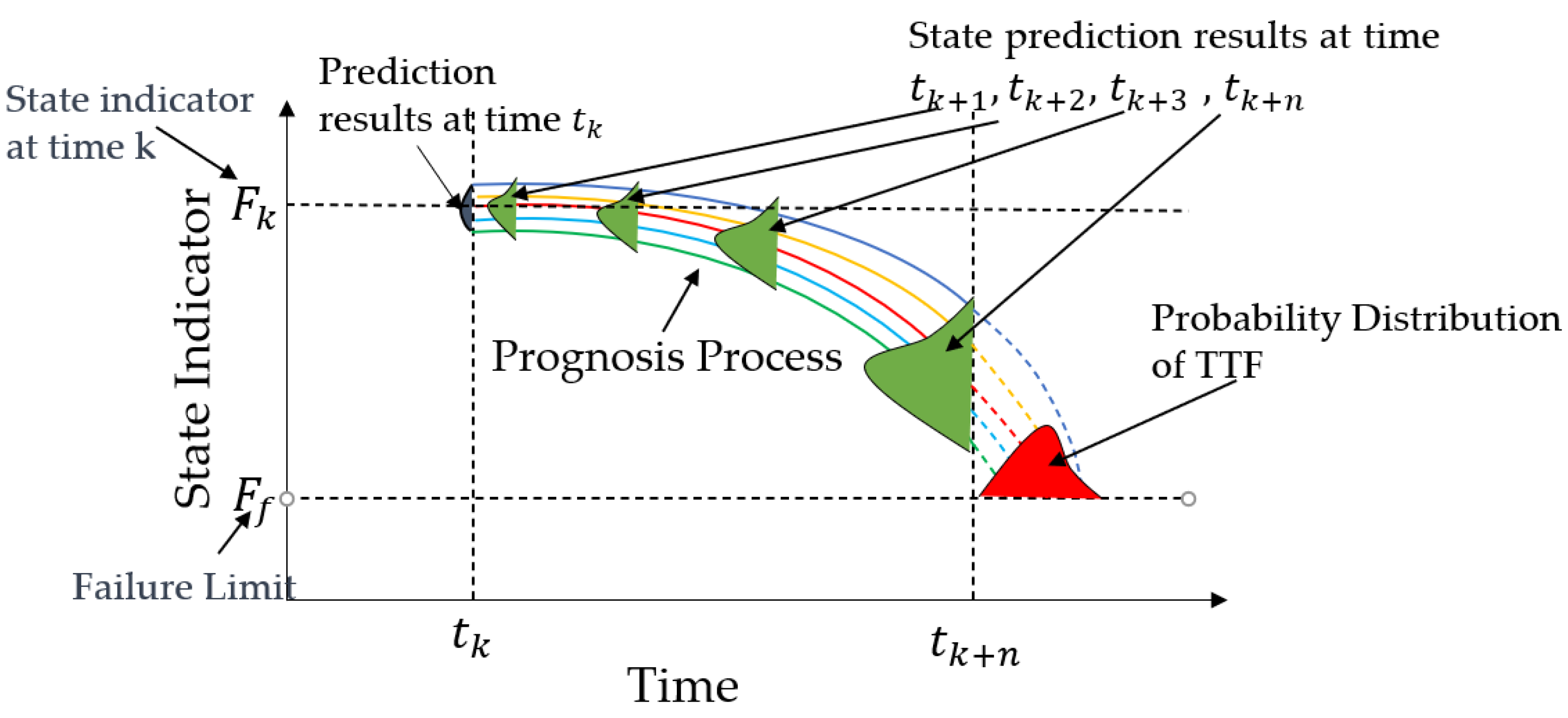
The purpose of life prognosis is to obtain the future development of the degradation process and then calculate the expected time to failure (TTF) for the state indicators to reach the failure threshold. In the prognosis, the estimation results at the current time are used as the initial values. During the prognosis stage, a multistep prognosis approach is used to recursively obtain the predicted values of state indicators at any future time, and the prognosis process continues until the predicted value of the state indicator exceeds the preset failure limit. Afterward, based on the prognosis results, the final TTF probability distribution can be obtained. As shown in Figure 6, the green probability distribution presents the state prognosis results at times t_k+1, t_k+2, and t_k+3, and the red region represents the corresponding TTF probability distribution. The calculation process for a multistep prognosis can be expressed as follows:

$$p(x_{t+m}^e|y_{1:t})=p(x_t^e|y_{1:t})p(x_{t+1}^e|x_t^e)d{x}_t^{e}p(x_{t+2}^e|x_{t+1}^e)d{x}_{t+1}^e\cdots p(x_{t+m}^e|x_{t+m-1}^e)d{x}_{t+m-1}^e$$

(25)

where $p(x_{t+m}^e|y_{1:t})$ represents the probability distribution of the state after the next m steps, $p(x_{t+1}^e|x_t^e)$, $p(x_{t+2}^e|x_{t+1}^e)$, and $p(x_{t+p}^e|x_{t+p-1}^e)$ represent the state transition process of the prognosis process. Afterward, the distribution of TTF is calculated based on the preset failure limit. The calculation process can be represented as follows:

$$p_f(t)=p(f|x_t>F_f)={\displaystyle \sum _{i=1}^N\mathrm{Pr}(f|}{x}_t^i>F_f)w_t^i$$

(26)

where $p_f(t)$ represents the failure probability at time t, $F_f$ represents the failure threshold.

In multistep prognosis, the future observed values are not available in advance, making it impossible to perform posterior updates on the predicted values. As the prognosis progresses, the uncertain parameters in the model accumulate during the iteration process, which can impact the effectiveness of the prognosis results. The above analysis indicates that uncertain parameters have a significant impact on prognosis results, but the classic modeling method lacks theoretical descriptions of uncertainties, failing to provide appropriate values for uncertain parameters. Manual adjustments of parameter values are necessary to obtain acceptable results. Therefore, to address this issue, a differential modeling method can be utilized to accurately model the heat transfer process of condenser fouling, effectively quantify the uncertain parameters in the process, and maximize the effectiveness of the prognosis results.

Describe the change in state between any two adjacent moments using the Differential law:

$$\frac{x_{t+1}-x_t}{(t+1)-t}=g^{\prime }(x_t,t)+{\omega }_t$$

(27)

where g′(·) is the differential equation, and ${\omega }_t$ represents the differential uncertainty present in the process. Transforming it into the state transition equation, the resulting state space model based on differential modeling is as follows:

$$x_{t+1}=g^{\prime }(x_t,t)+x_t+{\omega }_t$$

(28)

$$y_t=x_t+{\nu }_t$$

(29)

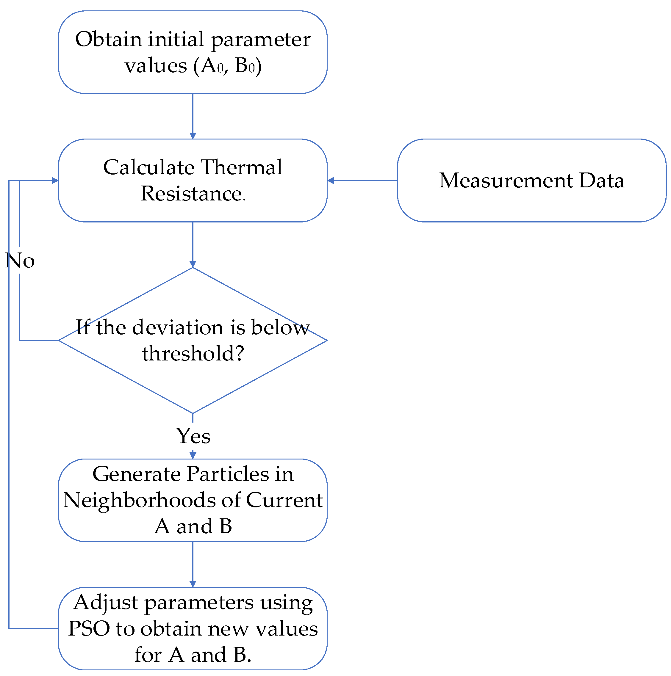
The above equation utilizes the differential law to describe the actual dynamic process. After performing the differential operation on the original fault data, fitting the obtained differential feature allows for the determination of model parameters corresponding to g′(·) and uncertainty parameters corresponding to ${\omega }_t$. The steps for model establishment and obtaining parameter values are as follows:

• Data smoothing: Due to the influence of internal components, circuit elements, and external factors such as human or environmental interference, actual equipment often exhibits noise when using sensors to collect performance parameters. The presence of random noise makes it difficult to directly and accurately identify valid differential laws through differential operations. Therefore, at the beginning of establishing the differential model, it is necessary to smooth the data to eliminate the random noise present in the raw data and obtain a smoothed dataset that still retains the primary characteristic information from the original data.
• Extracting and quantifying state observation uncertainty: Subtract the smoothed data from the original data to obtain the removed random noise and treat it as the uncertainty of the state observation process. According to its distribution, it is possible to quantify ${\nu }_t$ and determine the specific values.
• Extracting dynamic differential features: The dataset obtained after smoothing, which retains the main information of the original data, can be utilized to construct a differential model. Performing a differential operation on the values corresponding to any two adjacent moments with a fixed interval, and then fitting the obtained differential data to construct the corresponding differential model g′(·).
• Extracting and quantifying the uncertainty in the state transition: Using a similar method as mentioned above, extract the uncertainty in the state transition process. Subtract the results of the differential model from the actual differential data, and determine the value of ${\omega }_t$ based on the distribution of the differences.
• Establishing a state transition model: Based on the obtained differential model g′(·), substitute it into Equation (28) to establish the corresponding state-space model. Afterward, the state space model can be combined with the Particle Filtering algorithm to predict the future state and RUL of the system.

4. Case Study

In the previous section, the theoretical aspects involved were explained. The following is a specific case to illustrate the above content.

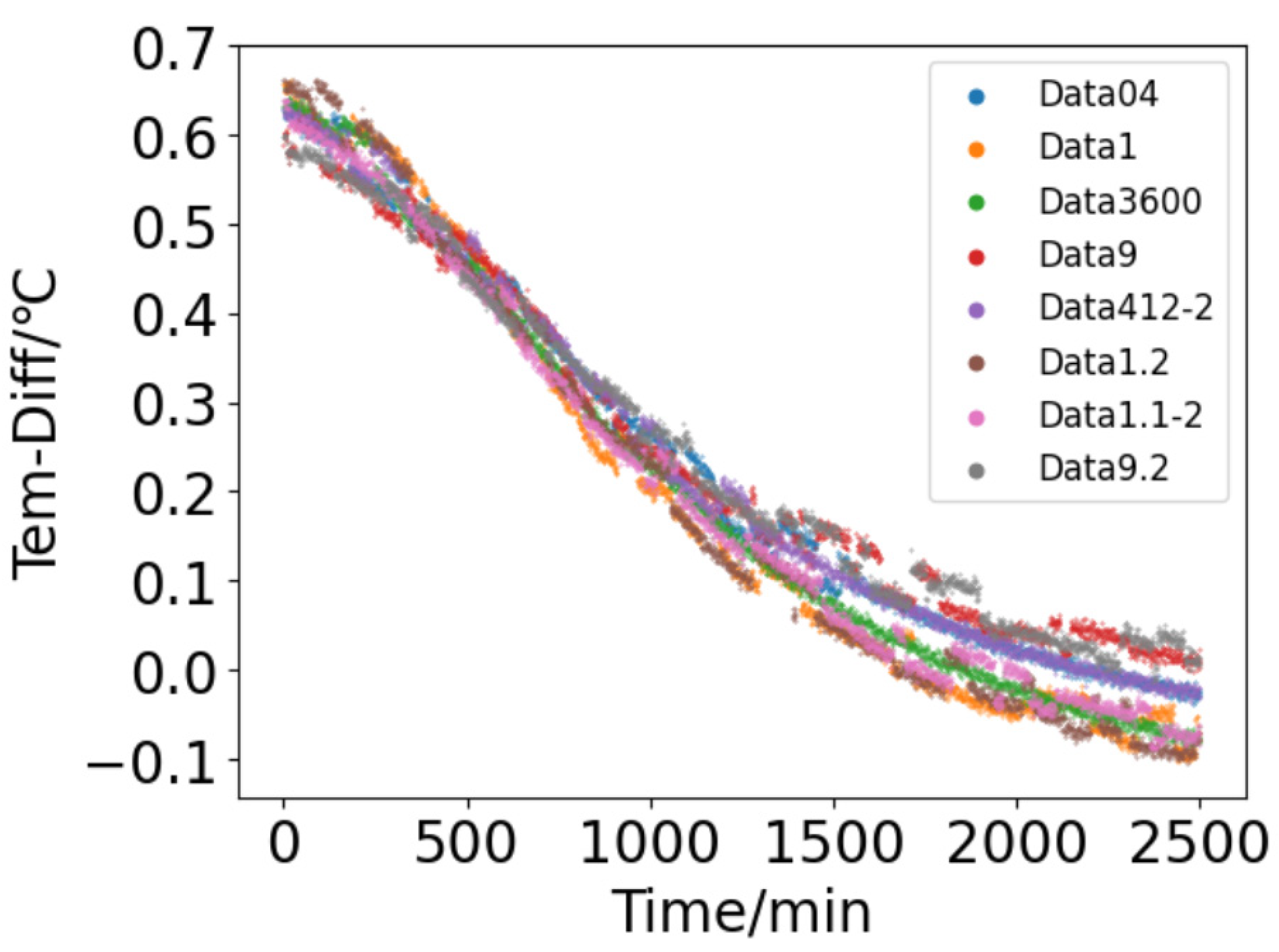
Based on the methods mentioned in Section 2, the inlet and outlet temperatures of cooling water under the fouling fault can be obtained through simulation tools. The established simulation model has a condenser inlet temperature of 48.5 °C, a cooling water inlet temperature of 28 °C, and a cooling water flow rate of 129 kg/s. Under the condition of not changing the trends of fouling thermal resistance, adjust the size of thermal resistance in a certain proportion to simulate different fault scenarios and obtain multiple sets of fault data. To simulate the temperature data collected by the actual temperature sensor, noise is added to the calculated temperature data from the simulation model. The resulting data is shown in Figure 7. The vertical axis represents the temperature difference between the inlet and outlet, measured in degrees Celsius (°C). (The data has been normalized.) The horizontal axis represents time, and the curve represents the changes of multiple sets of temperature difference data over time. The figure contains 8 sets of fault data under different conditions, labeled as DATA04, Data1, Data3600, Data9, Data412-2, Data1.2, Data1.1-2, and Data9.2.

For the heat exchange process of a condenser, the efficiency of the heat exchanger is defined as [41]:

$$\epsilon =\frac{{(t\prime -t″)}_{\max }}{t_1\prime -t_2\prime }$$

(30)

The denominator represents the maximum temperature difference between the fluids in the heat exchanger, while the numerator represents the larger of the actual temperature differences between the cold or hot fluids in the heat exchanger.

In the heat exchange process of the condenser mentioned above, the temperature difference of the cooling water plays a crucial role in determining the heat exchange efficiency. Specifically, the numerator of the heat exchange efficiency equation represents the temperature difference between the inlet and outlet of the cooling water. When the temperatures of the inlet steam and the inlet cooling water remain relatively constant, the heat exchange efficiency is directly influenced by the temperature difference between the inlet and outlet of the cooling water. As the temperature difference decreases, the heat exchange efficiency also decreases proportionally. To establish a failure limit for the condenser, a certain value $F_f$ can be set as a threshold for the temperature difference. When the temperature difference is below $F_f$, the heat exchange efficiency also decreases to a certain extent, indicating a potential failure condition. The deposition of fouling will reduce the temperature difference between the inlet and outlet of the cooling water, which will reduce the heat transfer efficiency. Therefore, the change in temperature difference between the inlet and outlet of the cooling water can, to some extent, characterize the impact of fouling on the heat transfer process of the condenser.

4.1. Classic Modeling Method

For the classic modeling method, using a portion of the acquired fault data as the training set, the classic curve fitting method is employed to model the data. The mathematical form of the polynomial model can be expressed as follows:

$$\Delta T=a_0+a_{1}t+a_2{t}^2+a_3{t}^3+a_4{t}^4$$

(31)

where $\Delta T$ is the temperature difference between the inlet and outlet of the cooling water, and a = [a₀, a₁, a₂, a₃, a₄] are the coefficients of the model. Four datasets (Data04, Data3600, Data9, and Data1) from the fault data were selected as the training set, and the fitting results are presented in Figure 8. The axes in Figure 8 have the same meaning as in Figure 7, and the black solid line represents the results obtained from the fitted model calculation. From the figure, it can be observed that the polynomial model fits the actual values very well, indicating that the fitted model effectively describes the changing process of the temperature difference between the inlet and outlet of cooling water.

Equation (15) represents the recursive relationship between states, so it is necessary to perform certain transformations on Equation (31). Firstly, for the temperature difference $\Delta T_{t+1}$ at time t + 1, it can be expressed as follows:

$$\Delta T_{t+1}=a_0+a_1(t+1)+a_2{(t+1)}^2+a_3{(t+1)}^3+a_4{(t+1)}^4$$

(32)

After the mathematical transformation of Equations (31) and (32), the following recursive relation can be obtained:

$$\Delta T_{t+1}=\Delta T+a_1+a_2(2t+1)+a_3(3t^2+3t+1)+a_4(4t^3+6t^2+4t+1)$$

(33)

Then, incorporating the uncertain parameter in the model, the state space model based on the polynomial model can be expressed as follows:

$$x_{t+1}=x_t+a_1+a_2(2t+1)+a_3(3t^2+3t+1)+a_4(4t^3+6t^2+4t+1)+w_t$$

(34)

$$y_t=x_t+{\nu }_t$$

(35)

where $w_t\sim N\left(0,{\sigma }^2\left(w_t\right)\right)$ and ${\nu }_t\sim N\left(0,{\sigma }^2\left({\nu }_t\right)\right)$ are Gaussian noises with zero mean and standard deviations of $\sigma \left(w_t\right)$ and $\sigma \left({\nu }_t\right)$, respectively.

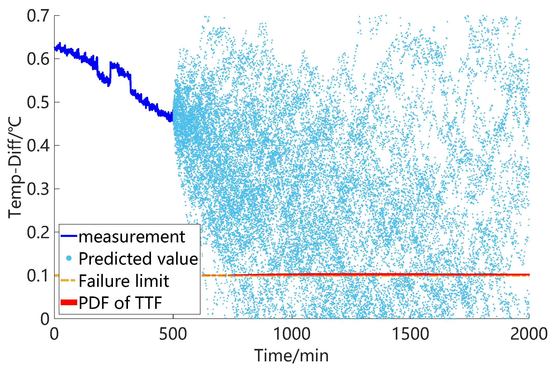
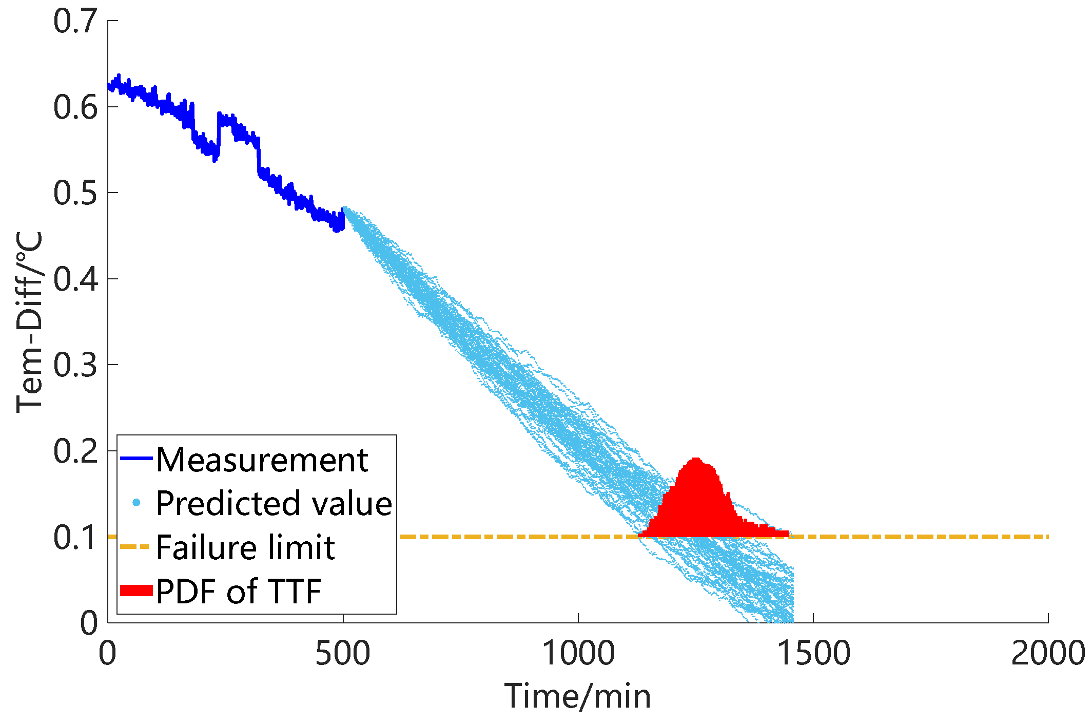
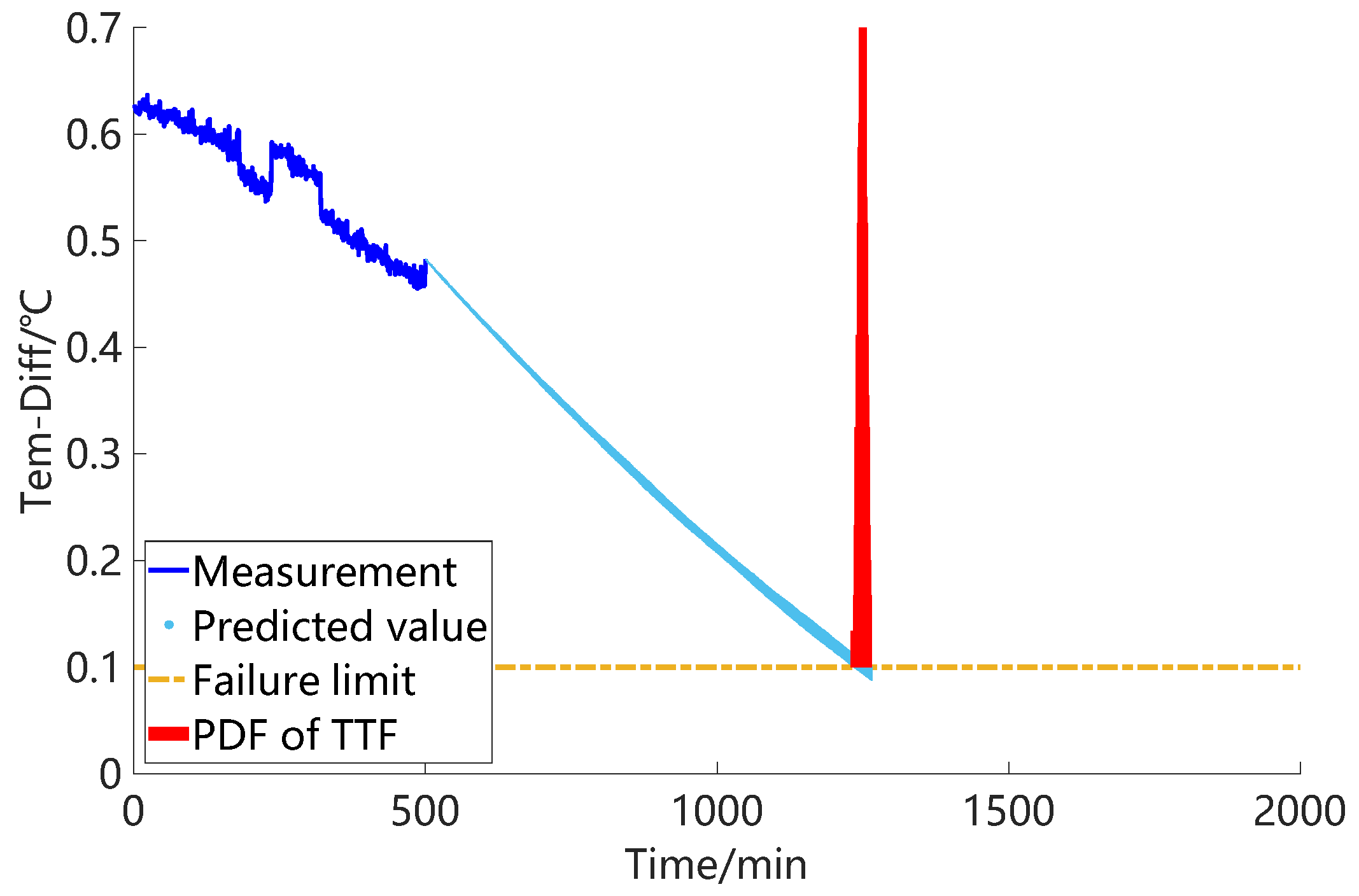
After establishing a suitable state space model, particle filter algorithms can be combined to predict the future development status of state indicators. Based on the significant impact of uncertain parameters on the prognosis results, it is necessary to make reasonable choices for their values. According to the modeling process mentioned above, it can be seen that the classic modeling method lacks a theoretical description and analysis of uncertain parameter values, and the parameter settings are often subjective. As shown in Figure 9, Figure 10 and Figure 11, the test results obtained by using different uncertain parameters for prognosis are shown. The model parameters (a= [a₀, a₁, a₂, a₃, a₄]) are kept constant, and the standard deviation of the difference between the curve fitting result and the actual data is 0.0359. Based on their order of magnitude, three levels of uncertain parameters are selected for testing: 0.01, 0.001, and 0.0001. The predicted results are presented in Figure 9, Figure 10 and Figure 11, respectively. The dark blue line in the figure represents the measurement data, the light blue dots represent the predicted results obtained after each particle filter, and the red area represents the probability distribution of TTF. Through the comparison of the three results, it can be observed that reducing the uncertain parameters has a significant impact on the prognosis results. As the uncertain parameters decrease, the predicted values of the state indicators become more concentrated, indicating higher confidence in the prognosis. Additionally, the confidence interval of the TTF probability distribution also decreases, indicating increased accuracy.

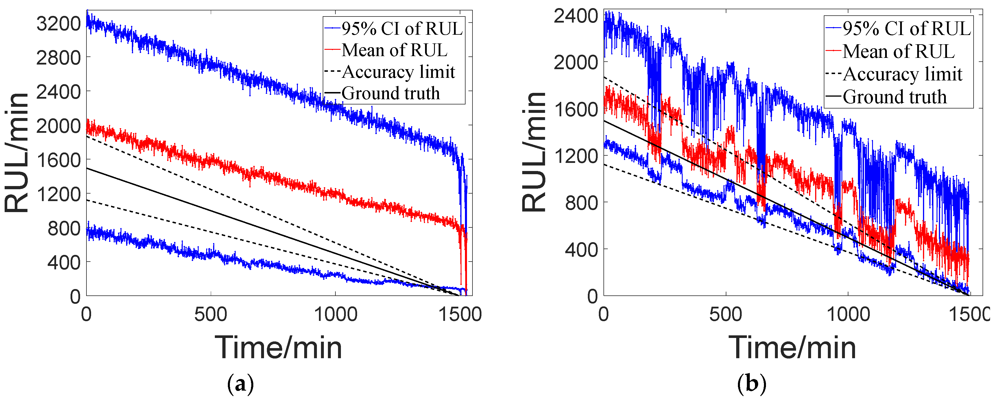
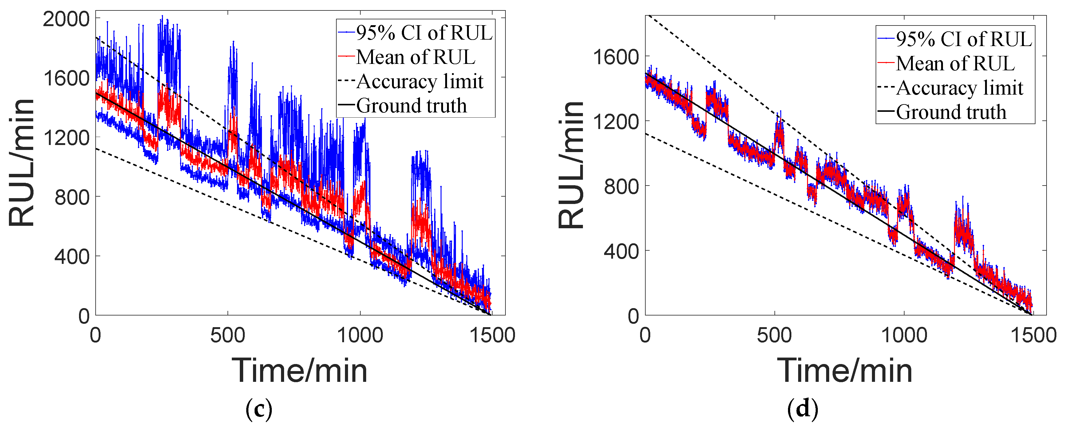
To provide a better reference for operation and maintenance, the corresponding RUL can be predicted and calculated. RUL refers to the duration from the predicted start time until the TTF is reached. In practical applications, prognoses are often initiated when the system’s performance has degraded significantly. This is conducted by setting an initial threshold to determine whether performance deterioration has occurred. This threshold determines the starting prediction time, denoted as T_s. However, for fouling faults in the condenser, the accumulation of fouling in the coolant occurs continuously once the condenser is in use. Therefore, in the case of condenser fouling faults, T_s can be set to 0, indicating that predictions can be made from the beginning of the system’s operation. The results of the corresponding RUL obtained through predictive operations throughout the entire cycle under various settings of uncertain parameters are depicted in Figure 12. In the figure, the solid black line represents the true values of the RUL. The black dashed line represents the upper and lower limits of the error (with α set to 0.25). The red line represents the mean of the prognosis results, while the blue line represents the range of the results. Based on the standard deviation (0.0359) of the above fitting results, the prognosis results obtained by setting uncertain parameters (0.01) of the same magnitude are poor, and satisfactory prognosis results cannot be achieved. As the uncertain parameters decrease, there is an improvement in the predictive performance of the RUL.

Two performance evaluation indicators, CMAPE (cumulative mean absolute percentage error) and CMPCIL (cumulative mean percentage 95% confidence interval length), are employed to assess the overall performance of the prognosis results throughout the entire cycle. CMAPE takes into account the temporal accuracy of the prognosis results, while CMPCIL considers the temporal precision of the prognosis results. The calculation methods for both are as follows:

$$CMAPE=\frac{1}{E-S+1}{\displaystyle \sum _{i=s}^E\frac{\left|r\prime (t_i)-r(t_i)\right|}{r\prime (t_i)}}$$

(36)

$$CMPCIL=\frac{1}{E-S+1}{\displaystyle \sum _{i=S}^E\frac{\sup (CI(t_i))-\inf ((CI(t_i))}{r\prime (t_i)}}$$

(37)

where $t_s$ is the starting time of the prognosis, $t_E$ is the end time of the prognosis, $r\prime (t_i)$ represents the RUL result obtained after executing the prognosis at time $t_i$, $r(t_i)$ represents the actual RUL result at time $t_i$, $\sup (CI(t_i))$ represents the upper limit of the confidence interval for the prognosis result at time $t_i$, $\inf ((CI(t_i))$ represents the lower limit of the confidence interval for the prognosis result at time $t_i$. The two evaluation indicators, CMAPE and CMPCIL, consider all prognosis results from the start to the end of the prognosis phase and are subjected to arithmetic averaging.

The performance testing was conducted on multiple datasets, and the calculated results for the indicators are shown in

Table 1. Calculation results of performance evaluation indicators for the prognosis method based on classic modeling.

Uncertain Parameter		0.01	0.001	0.0005	0.0001	0.00005
CMAPE	Data9.2	1.58	1.96	1.42	1.18	1.16
	Data412-2	4.07	1.50	0.51	0.39	0.39
	Data1.2	5.55	0.80	0.57	0.50	0.50
	Data1.1-2	4.35	0.51	0.25	0.22	0.22
average		3.89	1.19	0.69	0.57	0.57
CMPCIL	Data9.2	4.32	3.72	1.88	0.42	0.21
	Data412-2	8.94	4.03	0.91	0.13	0.07
	Data1.2	11.48	1.57	0.60	0.10	0.05
	Data1.1-2	9.44	1.74	0.48	0.09	0.04
average		8.55	2.77	0.97	0.19	0.09

. The table showcases the variation in prognosis performance as the values of ${\nu }_t$ and $w_t$ change. The test results from multiple datasets further indicate that setting uncertain parameters based on the standard deviation of the curve fitting results does not yield effective results. As the parameters decrease, CMAPE and CMPCIL show significant improvements, indicating a substantial enhancement in prognosis performance. However, when the parameters reach a sufficiently low value, further reducing the settings only leads to improvements in precision but marginal gains in the accuracy of the prognosis results. The aforementioned results indicate that, when using the prognosis method based on classic modeling, the setting of uncertain parameters has a significant impact on the prognosis results. But obtaining appropriate parameter values during the modeling process is not directly achievable, and it requires manual adjustment to obtain suitable values.

4.2. Differential Modeling Method

According to the performance test results, it is evident that the setting of uncertain parameters significantly affects the prognosis’s performance. Prognosis methods based on classic modeling can achieve acceptable results when uncertain parameters are appropriately configured. Indeed, the process of obtaining appropriate values for uncertain parameters often involves multiple manual adjustments and lacks a clear determination of the optimal values and quantification criteria for these parameters. The differential modeling method can effectively address such issues. Follow the differential modeling steps mentioned in the previous section to establish the differential model and quantify the uncertain parameters.

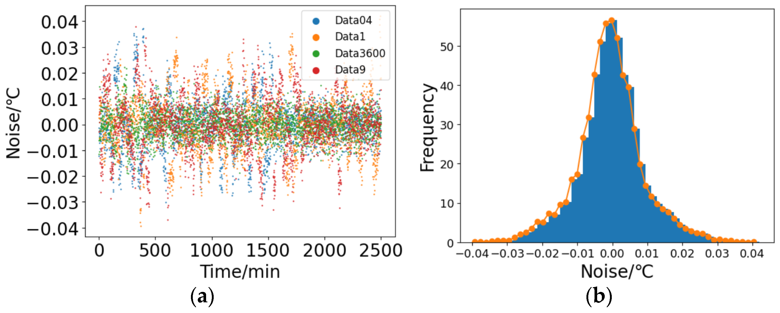
According to Step 1, the Savitzky–Golay algorithm is used to smooth the data. Random noise in the original data can be eliminated. The obtained random noise is shown in Figure 13a. The vertical axis in the figure represents the magnitude of the noise. Figure 13b shows the statistical distribution of the noise, and it can be seen that it resembles a Gaussian distribution. The “Frequency” axis represents the frequency of the noise in the statistical sense. Based on its distribution and the standard deviation calculated as 0.0094, $\sigma ({\nu }_t)$ can be set as this standard deviation. i.e., ${\nu }_t~N\left(0,{0.0094}^2\right)$. 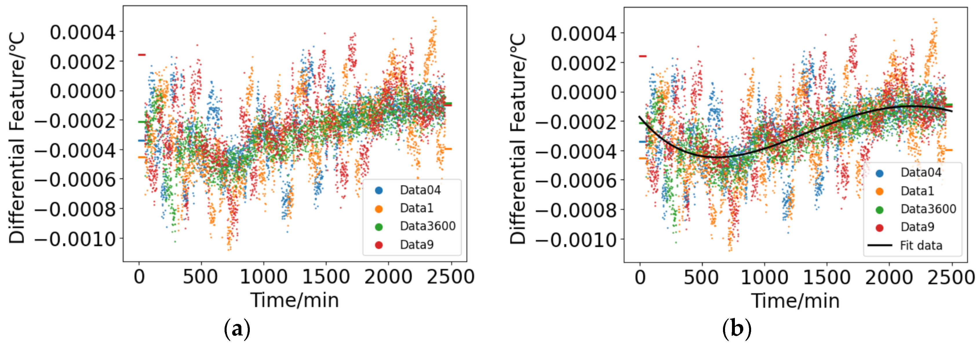According to Step 3, the differential operation is performed on the smoothed dataset, and the results are shown in Figure 14a. The vertical axis in the figure represents the magnitude of the differential feature. The distribution range of this is primarily within [0.0002, −0.001]. This range is smaller in magnitude compared to the noise depicted in Figure 13a, indicating that the differential feature is susceptible to being overwhelmed by random noise, making it challenging to directly extract it. From the figure, it can be seen that the differential feature exhibits a clear time-varying pattern. Therefore, it is possible to perform curve fitting on the differential data to construct a corresponding differential model. The results of this modeling process are illustrated in Figure 14b. The black curve in the figure represents the fitting results of the differential model.

The mathematical model obtained by fitting the differential feature using a 4-order polynomial model is as follows:

$$g\prime (x_t,t)=b_0+b_{1}t+b_2{t}^{{}_2}+b_3{t}^{{}_3}+b_4{t}^4$$

(38)

where b = [b₀, b₁, b₂, b₃, b₄] are the coefficients of the differential model.

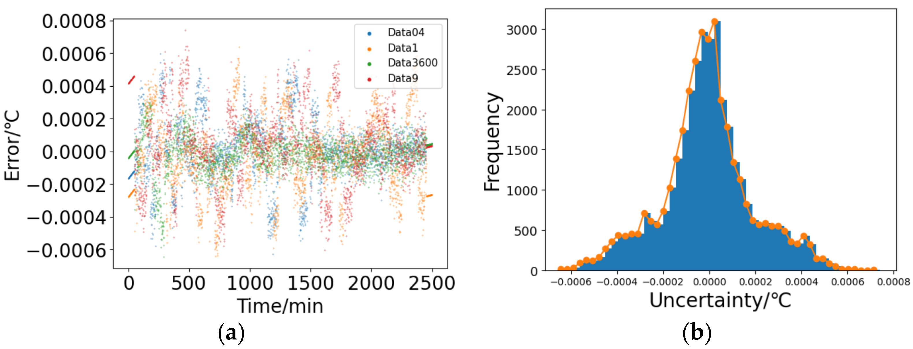
The results obtained by subtracting the fitted data from the original data in Figure 14b are depicted in Figure 15a. The vertical axis in the figure represents the magnitude of the error between the calculated results of the differential model and the actual differential feature. Figure 15b shows the statistical distribution of the error, where the “uncertainty” axis also represents “error/°C”. Similarly, based on its distribution, it closely resembles a Gaussian distribution. Therefore, it can be treated as the uncertainty in the state transition process, and its standard deviation is calculated to be $1.98\times {10}^{-4}$. i.e.,${\omega }_t~N\left(0,{\left(1.98\times {10}^{-4}\right)}^2\right)$. 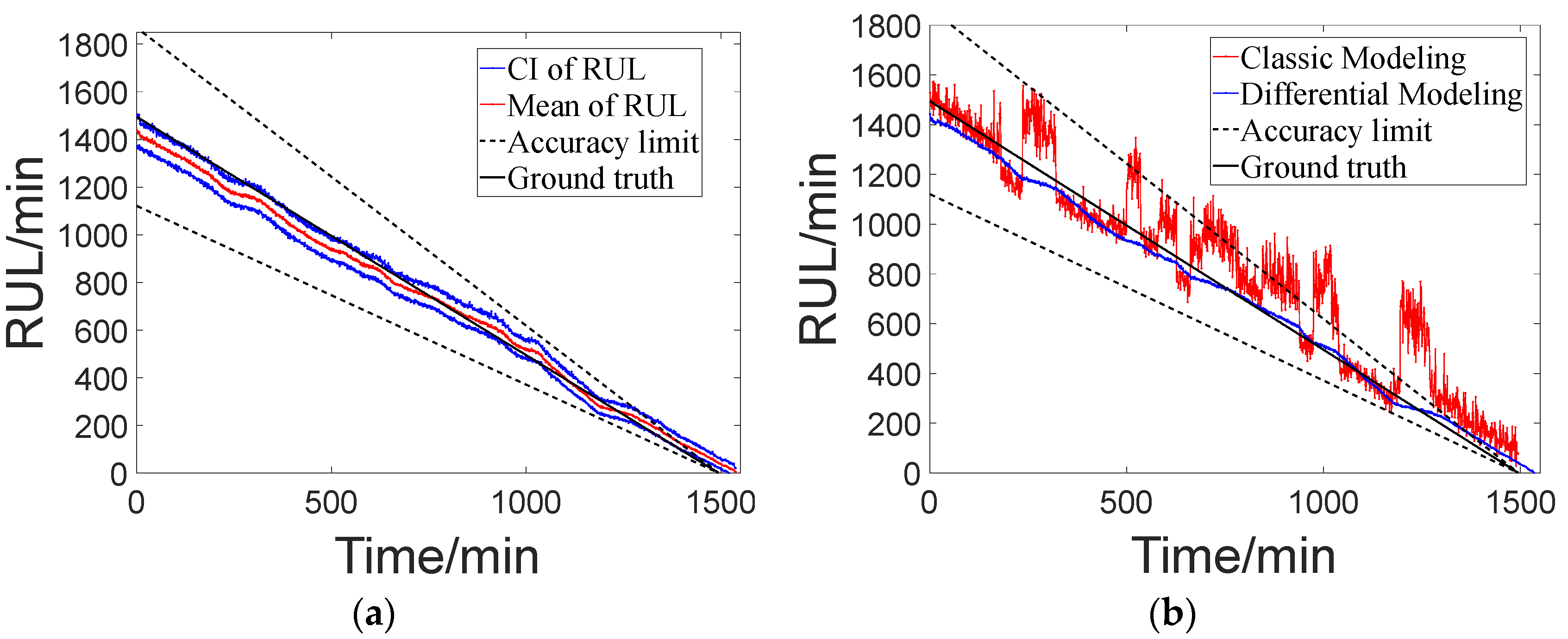Based on the fitted g′(·), the corresponding state transition model is established, and then combined with particle filtering for prognosis. The predicted RUL results are shown in Figure 16a.

Compared with the classic method, the prognosis method based on differential modeling can simultaneously obtain the specific settings of model parameters and uncertain parameters. Based on the comparison of the prognosis results in Figure 16b, the red line represents the prognosis results based on classic modeling with uncertain parameters of 0.0005, while the blue line represents the prognosis results based on differential modeling. The latter demonstrates an advantage in terms of stability in the prognosis results. In prognosis results based on classic modeling, when dealing with data that contains noise, the final results often exhibit significant random fluctuations. Similarly, performance testing was conducted on multiple test datasets, and the evaluation indicator calculation results obtained are shown in

Table 2. Calculation results of performance evaluation indicators for the prognosis method based on differential modeling.

Indicator	Data9.2	Data412-2	Data1.2	Data1.1-2	Average
CMAPE	0.40	0.19	0.73	0.09	0.35
CMPCIL	0.21	0.18	0.21	0.13	0.18

. The best CMAPE reached 0.09, with an average value of 0.35. Compared to the classic modeling method, the accuracy of the prognosis results was further improved, and the best CMPCIL reached 0.13, with an average value of 0.18. Based on this, it can be seen that the prognosis method based on differential modeling can achieve superior results in the prognosis of condenser fouling. It possesses excellent modeling capabilities and effective management of uncertainties, eliminating the need for manual adjustment and optimization of parameters to obtain acceptable prediction performance.

5. Conclusions

According to the features of the digital twin being able to perform online parameter correction based on real-time measurement data, this paper adopts an empirical equation of fouling thermal resistance to reflect the basic law of fouling growth over time and then uses measured data to calibrate the model parameters online. This approach enables the establishment of a digital twin model for predicting condenser fouling thermal resistance. Set the fouling fault into the simulation loop of the condenser and obtain the fault data of the condenser heat transfer process, thus addressing the issue of insufficient data. Subsequent research on fault prognosis methods is conducted using this fault dataset. This paper adopts both the classic modeling method and the differential modeling method. In the classic modeling method, the values of uncertain parameters are subjectively set. Therefore, by setting different uncertain parameters, the impact of uncertainty on the prediction results is analyzed. The results indicate that the setting of uncertain parameters has a significant impact on the accuracy and precision of the prognosis results. However, classic methods often focus only on obtaining high-quality model parameters without systematically studying the issue of uncertain parameters. Although optimizing parameter settings manually can effectively improve prognosis performance, there are limitations to the extent to which parameter optimization can enhance the accuracy of the prognosis results when the parameters are sufficiently small. Furthermore, this method is unable to provide the optimal values for uncertain parameters and their quantification criteria. On the contrary, the differential modeling method can directly obtain the values of uncertain parameters during the modeling process while establishing a reliable model. Through the quantitative analysis of prognosis results using performance evaluation indicators such as CMAPE and CMPCIL, it is evident that the differential method achieves a lower average CMAPE value of 0.35, surpassing the performance of the prognosis method based on classic modeling. This indicates that the differential modeling method can achieve better results without the need for manual adjustments. Based on the above analysis, it can be concluded that the differential modeling method exhibits excellent overall performance when used for the prognosis of condenser fouling.