Analysis of Flow and Heat Transfer Characteristics and Multi-Objective Optimization for Sinusoidal PCHE

Abstract

A Printed Circuit Heat Exchanger (PCHE) is a compact heat exchanger with high temperature and pressure resistance and is considered one of the best choices for the recuperators in the Supercritical Carbon dioxide (S-CO₂) Brayton cycle. The flow and heat transfer performance of sinusoidal channel PCHE were analyzed and a second-order regression model was established based on the response surface method to improve the performance of the continuous channel PCHE. It was found that reducing the channel diameter, increasing the channel amplitude, and reducing the channel pitch can increase the average value of the heat transfer coefficient and pressure drop per unit length. Moreover, sensitivity coefficient analysis was used to investigate the influence of various structural parameters on flow performance, heat transfer performance, and comprehensive performance. In addition, the structure of the sinusoidal channel PCHE was optimized using a multi-objective genetic algorithm, and three sets of Pareto optimal solutions were obtained. The corresponding optimal channel diameter D, channel amplitude A, and channel pitch Lp were in the range of 1.0–1.7 mm, 2.4–3.0 mm, and 15.1–17.0 mm, respectively, which can provide theoretical basis for the design of PCHE.

1. Introduction

With the increasingly prominent global energy crisis, efficient energy utilization has attracted much attention. The S-CO₂ Brayton cycle has become a hotspot for research in recent years owing to the advantages of high system cycle efficiency, compact structure and wide environmental adaptability [1,2,3,4,5]. The recuperators are the most significant heat transfer component in the S-CO₂ Brayton cycle, substantially affecting system cycle efficiency and compactness. It needs to operate under the conditions of high pressure and temperature [4]. PCHE, with a high temperature and pressure resistance and compact structure, is considered one of the best candidates for recuperators in the S-CO₂ Brayton cycle [5].

PCHE, as a new type of plate heat exchanger, is manufactured using chemical etching and diffusion welding techniques. Due to these techniques, PCHE can withstand pressures above 90 MPa and temperatures above 900 °C, with a unit volume-to-surface area ratio of up to 2500 m²/m³ and a heat transfer efficiency above 98% [6]. Straight and zigzag channels are the first developed and produced structures of PCHE. Chen et al. [7] made two small-sized straight channel PCHEs and experimentally verified their feasibility in ultra-high-temperature reactors. Meshram et al. [8] compared the temperature and pressure drop changes along the high-temperature recuperator and low-temperature recuperator of zigzag channel PCHE and straight channel PCHE by numerical simulation. The results showed that the performance of heat transfer for the zigzag channel was better than that of the straight channel, but the flow performance was worse than that of the straight channel. Finally, friction factor f of straight channel and zigzag channel and empirical formulas for Nusselt number Nu were proposed. Li et al. [9] performed a numerical simulation of zigzag channel PCHE and straight channel PCHE, indicating that the flow resistance of straight channel PCHE was much lower than that of zigzag channel PCHE.

Although zigzag channel PCHE exhibits excellent performance of heat transfer, its pressure drop is higher than other types of flow channel [10,11,12]. To reduce the pressure loss, many scholars have proposed non-continuous channels such as S-shaped, airfoil-shaped, and C-shaped channels to reduce the pressure drop of PCHE [13,14,15,16,17,18,19]. Although these structures can effectively reduce the pressure drop of PCHE, they are too complicated to manufacture and difficult to put into practical production [20]. Some scholars have also optimized the continuous channels. Baik et al. [21] optimized the sharp corners of zigzag-type PCHE into smooth corners with a radius of 1 mm. The results showed the rounded structure can reduce the pressure drop by 40% to 65%. Abed et al. [22] researched the flow and heat transfer in a rectangular cross-section serpentine-channel PCHE by combining experimental and numerical simulation methods. It was affirmed that it enhanced the heat transfer ability and increased the pressure loss compared with the straight channel, thus obtaining improved comprehensive performance. Wen et al. [23] studied the performance of heat transfer and the characteristics of flow for sinusoidal corrugated channel PCHEs and found that increasing the amplitude and reducing the pitch can improve the heat transfer rate. The maximum rate of heat transfer calculated in the corrugated channel model was 33.74% higher than that of the straight channel. Bennett et al. [24] used a non-geometric resolution III experimental design method without replication to study the sensitivity of 20 operating conditions and geometric parameters of zigzag channel PCHE to fluid heat transfer and flow performance. It should be noted that the heat transfer and flow performance of zigzag channel PCHE were more sensitive to the changes in channel bending angle, mass flow rate, curvature radius. Jin et al. [25] selected the pitch, bending angle, and bending radius of the zigzag channel with chamfers as design variables, with heat transfer coefficient and pressure drop as optimization targets. The non-dominated sorting genetic algorithm II was used to optimize the performance of the PCHE. The results showed that both the bending angle and bending radius obviously affected the performance of PCHEs. However, the effect of pitch on the performance of the PCHE was relatively small. Du et al. [26] adopted the channel width, channel depth and aspect ratio of the rectangular section straight channel PCHE as the design variables, and the temperature drop, pressure drop and heat transfer coefficient as the objective function for multi-objective optimization by the method of the numerical simulation. It was concluded that the structure is optimal with a width of 0.29 mm and a depth of 0.39 mm.

As discussed above, many scholars have optimized their structures to improve the heat transfer and flow characteristics of continuous channel PCHEs. However, there are many performance evaluation indicators, and most studies still need to provide the optimal geometric parameters. There needs to be more research on optimizing the structure of sinusoidal PCHEs. The lack of structural parameters for sinusoidal channels makes it difficult to qualitatively and quantitatively analyze and optimize the performance of PCHEs. Therefore, this work analyzes the mechanism of the heat transfer and flow and structural optimization of the sinusoidal PCHE.

2. Numerical Methodology

2.1. Physical Model and Boundary Conditions

The flow channels of PCHE are very small, and in practical engineering, the number of flow channels in a PCHE can reach millions. Modeling and simulating the entire PCHE would require an unacceptable amount of computational resources and time, so simplification of the PCHE is necessary. Since the PCHE is made by welding a metal plate with identical flow channels, its geometric structure is periodic. Therefore, selecting one flow channel as a heat transfer unit for simulation can reflect the overall flow and heat transfer performance of the PCHE.

Figure 1 shows the overall schematic diagram of the heat transfer unit of the sinusoidal channel PCHE. The inlet and outlet face of the cold and hot fluids parallel the yoz plane, and the channel extends in the x-axis direction. To ensure uniform flow velocity at the inlet and prevent backflow at the outlet, a length of 100 mm extends the inlet and outlet ends, and the total length of the channel in the x-axis direction is 440 mm.

Figure 2 shows the structural parameters of the channel. A and Lp represent the amplitude and pitch of the channel, respectively, where A is set to 2 mm, and Lp is set to 20 mm. The structure of the sinusoidal channel is periodic in the x-axis, with a length of one pitch for each cycle, and there are a total of 12 cycles. Figure 3 shows a cross-sectional view at location B-B, where the diameter of the cold channel D is 1.5 mm, the unit width W is 2.5 mm, and the unit height H is 3.2 mm. The structural parameters of the cold and hot channels are equal to the distance from the left and right outer walls.

Figure 3 shows a cross-sectional view of section B-B. Periodic walls are set on the top and bottom outer walls and the left and right outer walls in the solid domain. The inlet condition is set as mass flow inlet, and the outlet condition is set as pressure outlet. CO₂ is chosen as the operating fluid for both hot and cold streams. The working conditions selected for numerical simulation in [8] are as follows: the inlet temperature T_{in, c} of the cold stream is 500 K, and the outlet pressure P_{out, c} is 22.5 MPa; the inlet temperature T_{in, h} of the hot stream is 730 K, and the outlet pressure P_{out, h} is 9 MPa. The CO₂ thermophysical parameters are obtained through NIST 9.0 software and fitted using the coefficients listed in

Table 1. CO₂ physical properties polynomial fitting results.

Work Condition	Polynomials
500–730 K, 22.5 MPa	$\begin{array}{}\rho =1770.81-6.11T+8.06\times {10}^{-3}{T}^2-3.72\times {10}^{-6}{T}^3\\ c_p=6682.71-23.61T+0.034T^2-1.65\times {10}^{-5}{T}^3\\ \lambda =0.10-3.28\times {10}^{-4}T+5.64\times {10}^{-7}{T}^2-2.72\times {10}^{-10}{T}^3\\ \lambda =7.84\times {10}^{-5}-2.50\times {10}^{-7}T+4.06\times {10}^{-10}{T}^2-1.98\times {10}^{-13}{T}^3\end{array}$
500–730 K, 9 MPa	$\begin{array}{}\rho =489.07-1.50T+0.0019T^2-8.30\times {10}^{-7}{T}^3\\ c_p=2485.77-6.37T+0.0098T-4.79\times {10}^{-6}{T}^3\\ \lambda =0.0087-3.05\times {10}^{-5}T+7.13\times {10}^{-8}{T}^2-3.97\times {10}^{-11}{T}^3\\ \lambda =7.76\times {10}^{-6}-2.93\times {10}^{-8}T+1.81\times {10}^{-11}{T}^2-1.41\times {10}^{-14}{T}^3\end{array}$

. Inconel 617 alloy is the solid material which can be used under extreme temperature and pressure conditions [8]. In the subsequent simulation process, Inconel 617 alloy is treated as a constant material property, with a density of 8360 kg/m³, a specific heat capacity at constant pressure of 417 J/(kg⋅K), and a thermal conductivity of 21 W/(m⋅K). Based on the operating conditions of the S-CO₂ Brayton cycle high-temperature recuperator [11,12], the Reynold number at the inlet of the cold stream is selected to be 10,000, 20,000, 30,000, 40,000 and 50,000 for simulation.

In addition, the SIMPLE algorithm is used to couple and solve the velocity and pressure terms in the simulation. The PRESTO! format is used for the pressure term and the second-order upwind discretization format is used for the momentum equation, energy equation, turbulent kinetic energy equation, and specific dissipation rate equation. The simulation is considered converged as the residual of the energy equation is less than 10⁻⁶, the residuals of the other equations are less than 10⁻³, and the pressure drop change at the inlet and outlet of CO₂ is within 0.01%.

2.2. Grid Independence Verification and Model Validation

The meshing component in the ANSYS Workbench platform is used with a multi-region approach to generate a hexahedral mesh for the geometric model. For the boundary layer mesh, the first layer thickness is set to 0.005 mm with five layers, and the boundary layer growth rate is set to 1.2. The mesh near the wall needs to satisfy y+ less than 1. The mesh details are shown in Figure 4.

The mesh independence is verified by selecting the results of cold stream heat transfer coefficient h and unit pressure drop Δp as the number of mesh nodes changes. Figure 5 shows the variation in cold stream heat transfer coefficient h and unit pressure drop Δp with increased mesh nodes. As the number of mesh nodes increases from 1,154,175 to 1,520,620, from 1,520,620 to 1,910,230, from 1,910,230 to 2,374,084, and from 2,374,084 to 3,129,565, the variation rates of heat transfer coefficient are 2.14%, 1.24%, 0.52%, and 0.15%, respectively. The variation rates of unit pressure drop are 1.97%, 1.06%, 0.41%, and 0.18%, respectively. It can be seen that when the number of mesh nodes reaches 2,374,084, the changes in cold stream heat transfer coefficient and unit pressure drop are minimal. Increasing the number of mesh nodes beyond this point will not affect the simulation results. Therefore, the number of mesh nodes is controlled at around 2,374,084.

To validate the reliability of the numerical simulation, this section conducts a simulation verification of the experiment conducted by Ishizuka et al. [27]. The experiment tested the flow and heat transfer of zigzag-type PCHE using S-CO₂ as the working fluid. The periodic boundary conditions are imposed on the top, bottom, left and right walls. The experimental results and the numerical simulation results are shown in

Table 2. Comparison between numerical calculation and experimental data.

	Experimental Data	Simulation Results	Error (%)
∆p in cold flow channel (kPa)	24.1	23.2	3.7
∆p in hot flow channel (kPa)	70.7	63.8	9.8
∆T in cold flow channel (K)	140.3	135.5	3.4
∆T in hot flow channel (K)	169.6	165.1	2.7

. The maximum error between the numerical simulation results and the experimental results for pressure drop is 9.8%, and for temperature difference is 3.4%. The error between the numerical simulation results and the experimental results is within 10%, proving the method’s reliability.

Table 3. Validation results of the simulation by Meshran.

	Experimental Data	Simulation Results	Error (%)
∆p in cold flow channel (kPa)	15.8	16.1	1.9
∆p in hot flow channel (kPa)	45.9	46.6	1.5
∆T in cold flow channel (K)	140.8	142.2	1.0
∆T in hot flow channel (K)	171.4	173.5	1.3

shows the validation of the simulation conducted by Meshran et al. [8]. The maximum error between the numerical simulation results and the literature for pressure drop is 1.9%, and for temperature difference is 1.3%. The reliability of the method is further proved.

2.3. Governing Equations and Parameter Definition

When using ANSYS Fluent 2021 software for solving, three fundamental equations must be satisfied:

Continuity equation (mass conservation equation):

$$\frac{\partial \left(\rho u_j\right)}{\partial x_j}=0$$

(1)

Conservation of momentum equation:

$$\rho \frac{\partial \left(u_i{u}_j\right)}{\partial x_j}=-\frac{\partial p_i}{\partial x_i}+\mu \frac{\partial }{\partial x_j}(\frac{\partial u_i}{\partial x_j}+\frac{\partial u_j}{\partial x_i}-\frac{2}{3}{\delta }_{ij}\frac{\partial u_k}{\partial x_k})$$

(2)

Conservation of energy equation:

$$\frac{\partial }{\partial x_j}\left[u_j\left(\rho E+p\right)\right]=\frac{\partial }{\partial x_j}\left(\left(k_f+k_t\right)\frac{\partial T}{\partial x_j}\right)$$

(3)

where k_f is the thermal conductivity of fluid; kt is the turbulent thermal conductivity; δ_ij is the Kronecker delta; ν is the kinematic viscosity; μ is the dynamic viscosity.

Palko [28] has shown that the SST k-ω model can accurately compute flow field information of supercritical fluids when a sufficient number of mesh nodes are provided, and this turbulence model has been widely used in various simulation calculations.

The equations for the turbulent kinetic energy and specific dissipation rate in the SST k-ω model are given by:

$$\frac{\partial \left(\rho k{u}_i\right)}{\partial x_i}=\frac{\partial }{\partial x_j}\left({\Gamma }_k\frac{\partial k}{\partial x_j}\right)+G_k-Y_k+S_k$$

(4)

$$\frac{\partial \left(\rho w{u}_i\right)}{\partial x_i}=\frac{\partial }{\partial x_j}\left({\Gamma }_w\frac{\partial w}{\partial x_j}\right)+G_w-Y_w+D_w+S_w$$

(5)

where G_k and G_w are the generation terms for turbulent kinetic energy and specific dissipation rate, respectively; Y_k and Y_w are the dissipation terms for turbulent kinetic energy and specific dissipation rate, respectively; D_w is the cross-diffusion term; S_k and S_w are the source terms defined according to the actual problem; Γ_k and Γ_w are the effective diffusion coefficients.

The effective diffusion coefficients Γ_k and Γ_w are expressed by the following formula:

$${\Gamma }_k=\mu +\frac{{\mu }_t}{{\sigma }_k}$$

(6)

$${\Gamma }_{\omega }=\mu +\frac{{\mu }_t}{{\sigma }_{\omega }}$$

(7)

where μ_t is the turbulent viscosity; σ_k and σ_ω are constants in the turbulence model.

The formula for hydraulic diameter D_h calculation is:

$$D_{\mathrm{h}}=\frac{4S}{L_{\mathrm{h}}}$$

(8)

where S is the cross-sectional area of the channel, in m²; L_h is the perimeter of the cross-sectional area of the channel, in m.

The formula for calculating Reynolds number Re of the fluid is:

$$Re=\frac{u\rho D_h}{\mu }$$

(9)

where u is the inlet velocity of the fluid, in m/s; μ is the dynamic viscosity of the fluid, in kg/(m⋅s).

The formula for calculating the logarithmic mean temperature difference ΔT_m is:

$$\mathsf{\Delta }{T}_m=\frac{\left(T_{\mathrm{w}}-T_{\mathrm{in}}\right)-\left(T_{\mathrm{w}}-T_{\mathrm{out}}\right)}{ln\left(\frac{T_{\mathrm{w}}-T_{\mathrm{in}}}{T_{\mathrm{w}}-T_{\mathrm{out}}}\right)}$$

(10)

where T_w is the average temperature of the wall, in K; T_in is the inlet temperature of the fluid, in K; T_out is the outlet temperature of the fluid, in K.

The formula for calculating the heat transfer coefficient h is:

$$h=\frac{q}{\mathsf{\Delta }{T}_m}$$

(11)

where q is the heat flux density, in W/(m²·K).

The formula for calculating the Nusselt number Nu is:

$$Nu=\frac{h{D}_h}{\lambda }$$

(12)

The formula for calculating the friction factor f is:

$$f=\frac{\mathsf{\Delta }p{D}_h}{2\rho u^{2}L}$$

(13)

where Δp is the pressure drop between the inlet and outlet of the fluid, in Pa.

The formula for calculating the overall performance parameter PEC [29] is:

$$PEC=\frac{Nu}{f^{\frac{1}{3}}}$$

(14)

3. Results and Discussion

3.1. Effects of Structural Parameters on the Performance of PCHE

In this section, when evaluating the influence of channel diameter on the performance of the PCHE, the channel amplitude is kept at 2 mm, and the channel pitch is 20 mm. When evaluating the effect of channel amplitude on the performance of the PCHE, the channel diameter is kept at 1.5 mm, and the channel pitch is 20 mm. When evaluating the impact of channel pitch on the performance of the PCHE, the channel diameter is kept at 1.5 mm, and the channel amplitude is 2 mm.

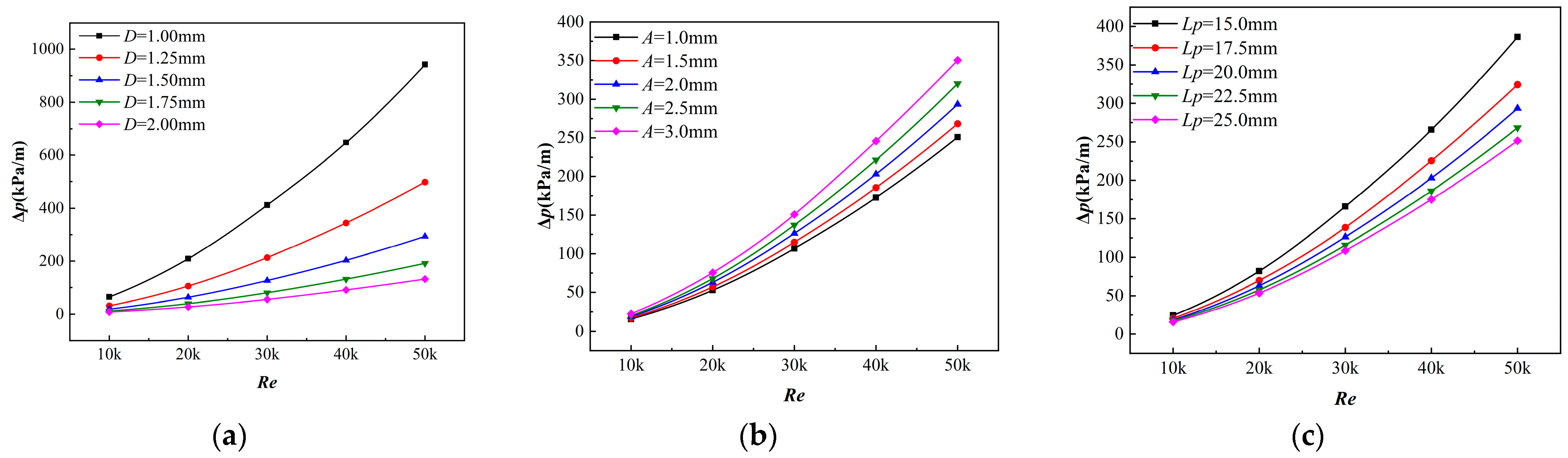
As shown in Figure 6 and Figure 7, with the increase in the Reynolds number, the influence of structural parameters on heat transfer coefficient and pressure drop gradually increases. Reducing the channel diameter, increasing the channel amplitude and decreasing the channel pitch of sinusoidal PCHE can increase the average value of heat transfer coefficient by up to 55.04%, 28.25%, and 16.56%, respectively, and increase the average value of unit pressure drop by up to 87.38%, 30.36%, and 35.08%, respectively. That indicates that the fluid in the channel with a smaller diameter has a higher velocity, higher turbulence kinetic energy, and more substantial heat transport capacity at the same inlet Reynolds number, which enhances the heat transfer performance but weakens the flow performance. The position sketch of the monitoring surface is shown in Figure 8. Plane 1, Plane 2 and Plane 3 are located at the fifth pitch, Plane 4 and Plane 5 are located at the sixth pitch. Axial velocity distribution under different channel amplitude in Figure 9. The larger amplitude of the channel is, the greater offset of the fluid velocity at the corner and the higher the degree of fluid disturbance is. Meanwhile, the flow separation phenomenon become more obvious, and the boundary layer is more significantly destroyed, which improves the heat transfer performance but weakens the flow performance. Axial velocity distribution under different channel pitch in Figure 10. For the channel with a smaller pitch, the frequency of fluid velocity offset is higher, the vortexes in the flow are more frequently destroyed and recombined, and the heat transfer rate is faster. However, the energy loss is more severe, which improves the heat transfer performance but weakens the flow performance.

As analyzed above, channels of different diameters have different velocities, which cause changes in flow and heat transfer performance. In order to understand the changes in flow and heat transfer performance of fluids under channels of different wave amplitudes and pitches more intuitively, the field synergy principle is used to explain the heat transfer improvement mechanism. According to the field synergy principle, the smaller the synergy angle, the better the synergy between velocity and temperature [30]. Forty-nine equidistant cross-sections are created along the direction of the cold fluid flow, with the first and last cross-sections corresponding to the inlet and outlet cross-sections of the cold fluid, respectively. The area-weighted average velocity and temperature synergy angle are used for calculation, with its formula given in Equation (15).

$$\alpha =arccos\frac{\left|\overline{U}\cdot \nabla \overline{T}\right|}{\left|\overline{U}\right|\cdot \left|\nabla \overline{T}\right|}$$

(15)

where $\overline{U}$ is the velocity vector, in m/s; $\nabla \overline{T}$ is the temperature gradient vector, in K.

As shown in Figure 11, the fluid velocity varies periodically along the flow channel, resulting in periodic changes in the synergy angle, which varies in a “W” shape. The smaller synergy angle is located at the peak or trough of the channel. Compared with channels with wave amplitudes of 1 mm and 2 mm, the velocity and temperature synergy angle in the channel with a wave amplitude of 3 mm decreased by 8.08% and 5.02%, respectively. Compared with channels with a pitch of 20 mm and 25 mm, the velocity and temperature synergy angle in the channel with a pitch of 15 mm decreased by 3.51% and 1.95%, respectively.

3.2. Sensitivity Analysis

The central composite face-centered design method in response surface analysis is used to design experiments for a three-factor, three-level scheme. The design results in a total of 15 experimental points. Each factor has three levels, with coded levels of −1, 0, and 1, respectively. The coding scheme and level values are shown in

Table 4. Coding scheme and value levels table.

Factor	Variable	Encoding and Proficiency Level
		−1	0	1
Diameter of the channel/mm	D	1.0	1.5	2.0
Amplitude of the channel/mm	A	1.0	2.0	3.0
Pitch of the channel/mm	Lp	15.0	20.0	25.0

.

Under the operating condition of the inlet Reynolds number of 30,000 for the hot and cold fluids, the ANSYS Fluent 2021 was used to simulate the 15 design points, and the corresponding objective function values were obtained. The specific experimental design scheme and results are shown in

Table 5. Experimental design points.

Cases	D (mm)	A (mm)	Lp (mm)	h (W/(m2∙K))	Δp (kPa/m)	PEC
1	1.0	1.0	15.0	7186.2	419.8	375.7
2	2.0	1.0	15.0	3657.1	55.9	374.9
3	1.0	3.0	15.0	10317.9	623.4	508.7
4	2.0	3.0	15.0	5523.8	108.6	492.5
5	1.0	1.0	25.0	6490.5	326.9	365.5
6	2.0	1.0	25.0	3254.3	39.9	370.7
7	1.0	3.0	25.0	8598.7	391.7	475.0
8	2.0	3.0	25.0	4222.4	54.7	452.3
9	1.0	2.0	20.0	8051.9	411.6	430.9
10	2.0	2.0	20.0	3972.0	55.0	417.7
11	1.5	1.0	20.0	4594.2	106.7	377.8
12	1.5	3.0	20.0	6177.5	150.9	478.3
13	1.5	2.0	15.0	6024.4	166. 0	444.1
14	1.5	2.0	25.0	5125.9	108.7	425.0
15	1.5	2.0	20.0	5365.8	126.3	427.1

.

Based on Table 4, the quadratic regression models for h, Δp, and PEC are expressed in Equations (16)–(18):

$$\begin{array}{c}h=16548.30-11326.30D+2653.62A-233.43Lp+2605.02DD\\ +43.94AA+3.97LpLp-601.30DA+35.54DLp-48.05ALp\end{array}$$

(16)

$$\begin{array}{c}\mathsf{\Delta }p=2057.42-1827.83D+179.58A-40.89Lp+433.95DD\\ +5.54AA+0.54LpLp-50.26DA+12.73DLp-4.41ALp\end{array}$$

(17)

$$\begin{array}{c}PEC=292.59+12.54D+100.37A+0.35Lp-10.83DA\\ -0.022DLp-1.49ALp\end{array}$$

(18)

In order to study the sensitivity of the three response factors (D, A, Lp) to the objective function, the value levels of the three response factors are uniformly ratioed, as shown in Equation (19). The ratioed response variable values can correspond to their original numerical values, and the specific correspondence can be referred to in

Table 6. Response factors and ratioed response variable values.

Cases	Factor	Encoding and Proficiency Level
		−1	0	1
1	D	1	1.5	2
2	Ratio-D	−1/3	0	1/3
3	A	1	2	3
4	Ratio-A	−0.5	0	0.5
5	Lp	15	20	25
6	Ratio-Lp	−0.25	0	0.25

.

$$Rati{o}_y=\frac{x-x_0}{x_0}$$

(19)

where x represents the numerical value of the response factor, and x₀ represents the value of the response factor at the 0 level.

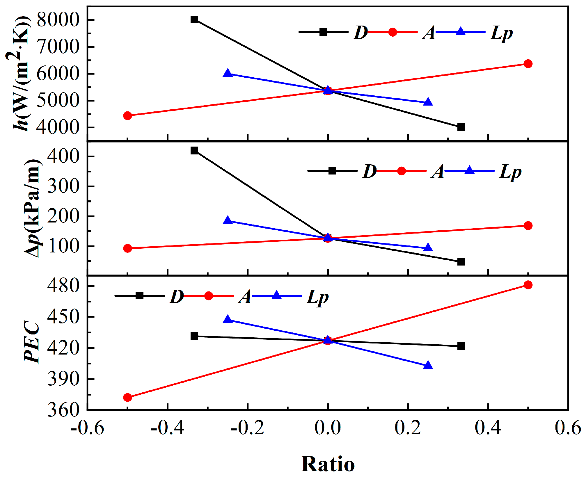
To study the sensitivity of each of the three objective functions to the response factors, the ratioed D, A, and Lp are used as the horizontal axis, and the three objective functions (h, Δp, and PEC) are used as the vertical axis, as shown in Figure 12. When studying the sensitivity of the objective function to a certain response factor, the other response factors should be kept at the 0 level, that is, D = 1.5 mm, A = 2 mm, Lp = 20 mm. The sensitivity of the response factor to the objective function depends on the slope of the line. If the slope is positive, the response factor is positively correlated with the objective function. If the slope is negative, the response factor is negatively correlated with the objective function. The larger the absolute value of the slope of the line, the higher the sensitivity of the response factor to the objective function.

From Figure 12, it can be seen that h has the highest sensitivity to D and the lowest sensitivity to Lp. In addition, D and Lp are negatively correlated with the heat transfer coefficient, while A and h are positively correlated. The relationships between h and A, Lp are linear, and the absolute value of the slope of the curve between h and D decreases with the increase of D, indicating that the sensitivity of h to D decreases with the increase of D. The sensitivity of Δp to D is significantly higher than that to A and Lp. Moreover, D and Lp are negatively correlated with Δp, while A is positively correlated. The sensitivity of Δp to D decreases with the increase of D. PEC has the highest sensitivity to A and is positively correlated, while it is negatively correlated with D and Lp. The slope between PEC and D is close to 0, indicating that the influence of D on PEC is small. The absolute value of the slope of the curve between PEC and Lp increases with the increase of Lp, indicating that the sensitivity of PEC to Lp increases with the increase of Lp.

To quantify the sensitivity of each response factor, the sensitivity coefficient is used as a measure of its size [31]. SC_y is used to represent the sensitivity coefficient of the objective function y (h, Δp, PEC) to the response factor x (D, A, Lp), and the calculation formula is shown in Equation (20).

$$S{C}_y=\frac{y-y_0/y_0}{x-x_0/x_0}$$

(20)

where y₀ represents the objective function value when encoded as 0, and x₀ represents the design variable value when encoded as 0.

The results are shown in

Table 7. Sensitivity coefficients of h, Δp, and PEC in sinusoidal PCHE.

Factor	SCh		SCΔp		SCPEC
	Range	Average	Range	Average	Range	Average
D	−1.481/−0.757	−1.119	−6.967/−1.867	−4.417	−0.030/−0.037	−0.034
A	0.345/0.375	0.360	0.534/0.672	0.603	0.257/0.252	0.255
Lp	−0.472/−0.330	−0.401	−1.834/−1.058	−1.446	−0.188/−0.228	−0.208

. The positive or negative sensitivity coefficient represents the correlation between the objective function and the response factor, positive for a positive correlation and unfavorable for a negative correlation, and the absolute value indicates the sensitivity level. For h, the sensitivity to D is the highest, 3.1 times and 2.8 times that of A and Lp, respectively. For Δp, the sensitivity to D is also the highest, 7.3 times and 3.1 times that of A and Lp, respectively. For PEC, the sensitivity to A is the highest, 7.5 times and 1.2 times that of D and Lp, respectively.

3.3. Multi-Objective Optimization

Based on the MATLAB 2018 platform, the non-dominated sorting genetic algorithm-II with elite strategy is used to optimize and solve the three objective functions (h, Δp, and PEC). The algorithm parameters are set as follows: the population size is 150, the maximum evolution generation is 300, the crossover probability is 80%, and the mutation probability is 5%.

Figure 13 shows the three-dimensional Pareto optimal solution diagram of the heat transfer performance, flow performance, and comprehensive performance of the sinusoidal PCHE. All points on the Pareto optimal boundary are the optimal solutions of multi-objective functions. This means that there is no second solution that can improve one function’s expected value without reducing the expected values of other functions. In other words, no solution can replace the solution on the Pareto optimal boundary.

The black dots in the Figure 13 represent the projection of the Pareto optimal boundary on each coordinate plane, as shown in Figure 14. Figure 14a represents the Pareto optimal boundary of h and Δp. It can be seen that point C is the Pareto optimal solution that balances the two objective functions of h and Δp. Figure 14b represents the Pareto optimal boundary of Δp and PEC. It can be seen that point B is the Pareto optimal solution that balances the two objectives of Δp and PEC. Figure 14c represents the Pareto optimal boundary of h and PEC. It can be seen that point D is the ideal point for both h and PEC, where both expected objectives are achieved optimally. Point A is the non-ideal point for both h and PEC, where both expected objectives are the worst. The objective function values and design variable values for points A, B, C, and D are shown in

Table 8. Four representative Pareto-optimal solutions.

	A	B	C	D
h (W/(m2∙K))	3540.0	5574.3	7552.8	10,274.4
Δp (kPa/m)	33.2	115.6	281.3	599.6
PEC	372.9	490.2	500.8	510.8
D (mm)	1.9	1.7	1.4	1.0
A (mm)	1.1	2.4	2.9	3.0
Lp (mm)	19.2	17.0	16.2	15.1

.

4. Conclusions

The sinusoidal channel PCHEs have the potential as a high-temperature recuperator of the S-CO₂ recompression Brayton cycle. In this paper, a three-dimensional numerical simulation was conducted to investigate the thermo-hydraulic performance of the sinusoidal channel PCHEs. Response surface analysis and multi-objective optimization were conducted on the structural parameters. The main conclusions are as follows:

(1)

Reducing the channel diameter, increasing the channel amplitude, and reducing the channel pitch can increase the average value of the heat transfer coefficient by a maximum of 55.04%, 28.25%, and 16.56%, respectively. It can increase the average value of the pressure drop per unit length by a maximum of 87.38%, 30.36%, and 35.08%, respectively.

(2)

The sensitivity of h to D is the highest, with a sensitivity coefficient equivalent to 3.1 times and 2.8 times that of A and Lp, respectively. The sensitivity of Δp to D is the highest, with a sensitivity coefficient equivalent to 7.3 times and 3.1 times that of A and Lp, respectively. The sensitivity of PEC to A is the highest, with a sensitivity coefficient equivalent to 7.5 times and 1.2 times that of D and Lp, respectively.

(3)

Based on the multi-objective genetic algorithm, a three-dimensional Pareto optimal solution set was obtained with h, Δp, and PEC as the optimization objectives for the sinusoidal PCHE. From the perspective of balancing each objective function, three sets of Pareto optimal solutions were obtained, corresponding to the optimal h, Δp, and PEC intervals of 5574.3–10,274.4 W/(m²∙K), 115.6–599.6 kPa/m, and 490.2–510.8, respectively; and the corresponding D, A, and Lp intervals were 1.0–1.7 mm, 2.4–3.0 mm, and 15.1–17.0 mm.

References

1. Cheng, W.L.; Huang, W.X.; Nian, Y.L. Global Parameter Optimization and Criterion Formula of Supercritical Carbon Dioxide Brayton Cycle with Recompression. Energ. Convers. Manag. 2017, 150, 669–677. [Google Scholar] [CrossRef]
2. Li, M.J.; Xu, J.L.; Cao, F.; Guo, J.; Tong, Z.; Zhu, H. The investigation of thermo-economic performance and conceptual design for the miniaturized lead-cooled fast reactor composing supercritical CO2 power cycle. Energy 2019, 173, 174–195. [Google Scholar] [CrossRef]
3. Fan, Z.L.; Zhou, Y.B.; Liu, D.H.; Wei, X.F.; Guo, Q.; Wang, K. Emission characteristics of nitrogen oxides from gas steam combined cycle unit. Chem. Ind. Eng. Prog. 2019, 38, 2056–2062. [Google Scholar]
4. Hejzlar, P.; Dostal, V.; Driscoll, M.J.; Dumaz, P. Ass of gas cooled fast reactor with indirect supercritical CO2 cycle. Nucl. Eng. Technol. 2006, 38, 109–118. [Google Scholar]
5. Mccormack, D. The application of printed circuit heat exchanger technology in the pebble bed modular reactor demonstration plan. In Proceedings of the ASME Turbo Expo 2001: Power for Land, Sea, and Air, New Orleans, LA, USA, 4–7 June 2001. [Google Scholar]
6. Oh, C.H.; Kim, E.S.; Patterson, M. Design option of heat exchanger for the next generation nuclear plant. J. Eng. Gas. Turb Power 2009, 132, 032903. [Google Scholar] [CrossRef] [Green Version]
7. Chen, M.; Sun, X.; Christensen, R.N.; Shi, S.; Skavdahl, I.; Utgikar, V.; Sabharwall, P. Experimental and numerical study of a printed circuit heat exchanger. Ann. Nucl. Energy 2016, 97, 221–231. [Google Scholar] [CrossRef] [Green Version]
8. Meshram, A.; Jaiswal, A.K.; Khivsara, S.D.; Ortega, J.D.; Ho, C.; Bapat, R.; Dutta, P. Modeling and analysis of a printed circuit heat exchanger for supercritical CO2 power cycle applications. Appl. Therm. Eng. 2016, 109, 861–870. [Google Scholar] [CrossRef] [Green Version]
9. Li, L.; Yang, J.; Ma, T. Study on high temperature heat transfer and resistance characteristics of channels in printed circuit boards. J. Eng. Thermophys. 2014, 35, 931–934. [Google Scholar]
10. Nikitin, K.; Kato, Y.; Ngo, L. Printed circuit heat exchanger thermal–hydraulic performance in supercritical CO2 experimental loop. Int. J. Refrig. 2006, 29, 807–814. [Google Scholar] [CrossRef]
11. Lee, S.W.; Shin, S.M.; Chung, S.K. Evaluation of thermal-hydraulic performance and economics of Printed Circuit Heat Exchanger (PCHE) for recuperators of Sodium-cooled Fast Reactors (SFRs) using CO2 and N2 as working fluids. Nucl. Eng. Technol. 2022, 54, 1874–1889. [Google Scholar] [CrossRef]
12. Jin, F.; Chen, D.; Hu, L.; Huang, Y.; Zeng, H.; Wang, J. Thermo-Hydraulic performance of printed circuit heat exchanger as precooler in supercritical CO2 Brayton cycle. Appl. Therm. Eng. 2022, 210, 118341. [Google Scholar] [CrossRef]
13. Tsuzuki, N.; Kato, Y.; Ishiduka, T. High performance printed circuit heat exchanger. Appl. Therm. Eng. 2007, 27, 1702–1707. [Google Scholar] [CrossRef]
14. Kim, W.; Baik, Y.J.; Jeon, S.; Jeon, D. A mathematical correlation for predicting the thermal performance of cross, parallel, and counterflow PCHEs. Int. J. Heat. Mass. Tran. 2017, 106, 1294–1302. [Google Scholar] [CrossRef]
15. Mohamed, R.A.; Kamel, A.K.; Muzamil, H.; Taher, L.; Sami, U.K.; Lioua, K. Effect of design parameters on passive control of heat transfer enhancement phenomenon in heat exchangers–A brief review. Case Stud. Therm. Eng. 2023, 43, 102674. [Google Scholar]
16. Haseeb, T.; Ramisha, S.; Muhammad, Z.U.K.; Kaouther, G.; Ali, A.; Sami, U.K.; Lioua, K. Effective waste heat recovery from engine exhaust using fin prolonged heat exchanger with graphene oxide nanoparticles. J. Indian Chem. Soc. 2023, 100, 100911. [Google Scholar]
17. Cui, X.Y.; Guo, J.F.; Huai, X.L.; Cheng, K.Y.; Zhang, H.Y.; Xiang, M.R. Numerical study on novel airfoil fins for printed circuit heat exchanger using supercritical CO2. Int. J. Heat. Mass. Tran. 2018, 121, 354–366. [Google Scholar] [CrossRef]
18. Zhu, C.Y.; Guo, Y.; Yang, H.Q.; Ding, B.; Duan, X.Y. Investigation of the flow and heat transfer characteristics of helium gas in printed circuit heat exchangers with asymmetrical airfoil fins. Appl. Therm. Eng. 2021, 186, 116478. [Google Scholar] [CrossRef]
19. Saeed, M.; Kim, M. Thermal-hydraulic analysis of sinusoidal fin-based printed circuit heat exchangers for supercritical CO2 Brayton cycle. Energ. Convers. Manag. 2019, 193, 124–139. [Google Scholar] [CrossRef]
20. Kwon, J.S.; Son, S.; Heo, J.Y.; Lee, J.I. Compact heat exchangers for supercritical CO2 power cycle application. Energ. Convers. Manag. 2020, 209, 112666. [Google Scholar] [CrossRef]
21. Baik, S.; Kim, S.G.; Lee, J.; Lee, J.I. Study on CO2—Water printed circuit heat exchanger performance operating under various CO₂ phases for S-CO₂ power cycle application. Appl. Therm. Eng. 2017, 113, 1536–1546. [Google Scholar] [CrossRef]
22. Abed, W.M.; Whalley, R.D.; Dennis, D.J.C.; Poole, R.J. Numerical and experimental investigation of heat transfer and fluid flow characteristics in a micro-scale serpentine channel. Int. J. Heat. Mass. Tran. 2015, 88, 790–802. [Google Scholar] [CrossRef]
23. Wen, Z.; Lv, Y.; Li, Q. Comparative study on flow and heat transfer characteristics of sinusoidal and zigzag channel printed circuit heat exchangers. Sci. China Technol. Sc. 2020, 63, 655–667. [Google Scholar] [CrossRef]
24. Bennett, K.; Chen, Y. A two-level Plackett-Burman non-geometric experimental design for main and two factor interaction sensitivity analysis of zigzag-channel PCHEs. TSEP 2019, 11, 167–194. [Google Scholar] [CrossRef]
25. Jin, F.; Chen, D.; Hu, L.; Huang, Y.; Bu, S. Optimization of zigzag parameters in printed circuit heat exchanger for supercritical CO2 Brayton cycle based on multi-objective genetic algorithm. Energ. Convers. Manag. 2022, 270, 116243. [Google Scholar] [CrossRef]
26. Du, M.; Meng, B.; Pan, F.; Wan, M. Optimized design of printed circuit board heat exchanger considering manufacturing constraints. J. Beijing Univ. Aeronaut. Astronaut. 2022, 48, 1994–2005. [Google Scholar]
27. Ishizuka, T.; Kato, Y.; Muto, Y.; Nikitin, K. Thermal-hydraulic characteristics of a printed circuit heat exchanger in a supercritical CO2 loop. Bull. Res. Lab. Nucl. React. 2006, 30, 109–116. [Google Scholar]
28. Palko, D.; Anglart, H. Theoretical and Numerical Study of Heat Transfer Deterioration in High Performance Light Water Reactor. Sci. Technol. Nucl. Install. 2008, 2008, 405072. [Google Scholar] [CrossRef] [Green Version]
29. Yang, G.; Shao, W.W. Research progress on heat exchanger structure and heat transfer correlation of printed circuit board. Chem. Ind. Eng. Prog. 2021, 40, 13–26. [Google Scholar]
30. Guo, Z.Y.; Tao, W.Q.; Shah, R.K. The field synergy (coordination) principle and its applications in enhancing single phase convective heat transfer. Int. J. Heat. Mass. Tran. 2005, 48, 1797–1807. [Google Scholar] [CrossRef]
31. Feng, Y.; Zhang, Y.; Li, B.; Yang, J.F.; Shi, Y. Sensitivity analysis and thermoeconomic comparison of ORCs (organic Rankine cycles) for low temperature waste heat recovery. Energy 2015, 82, 664–677. [Google Scholar] [CrossRef]
Figure 1. Overall schematic diagram.
Energies 16 05763 g001
Figure 2. Channel structure diagram.
Energies 16 05763 g002
Figure 3. Cross-sectional diagram at section B-B.
Energies 16 05763 g003
Figure 4. Schematic diagram of mesh division.
Energies 16 05763 g004
Figure 5. PCHE gird independence verification.
Energies 16 05763 g005
Figure 6. Heat transfer coefficient under different structural parameter. (a) Different diameters; (b) different amplitude; (c) different pitch.
Energies 16 05763 g006
Figure 7. Unit pressure drop under different structural parameters. (a) Different diameters; (b) different amplitude; (c) different pitch.
Energies 16 05763 g007
Figure 8. Schematic diagram of monitoring surfaces.
Energies 16 05763 g008
Figure 9. Axial velocity distribution under different channel amplitude.
Energies 16 05763 g009
Figure 10. Axial velocity distribution under different channel pitch.
Energies 16 05763 g010
Figure 11. Synergy angle for the PCHE with different wave amplitudes and pitches. (a) Different amplitude; (b) different pitch.
Energies 16 05763 g011
Figure 12. Sensitivity analysis of h, Δp, and PEC to each response factor in sinusoidal PCHE.
Energies 16 05763 g012
Figure 13. Pareto-optimal solution set of three objectives in sinusoidal PCHE displayed in a three-dimensional plot.
Energies 16 05763 g013
Figure 14. Pareto-optimal solution set displayed in a two-dimensional plot. (a) The Pareto-optimal frontier of h and Δp; (b) the Pareto-optimal frontier of Δp and PEC; (c) the Pareto-optimal frontier of h and PEC.
Energies 16 05763 g014