

Robust MPPT Control of Stand-Alone Photovoltaic Systems via Adaptive Self-Adjusting Fractional Order PID Controller

Abstract
:1. Introduction
1.1. Literature Review
1.2. Proposed Methodology
- (1)
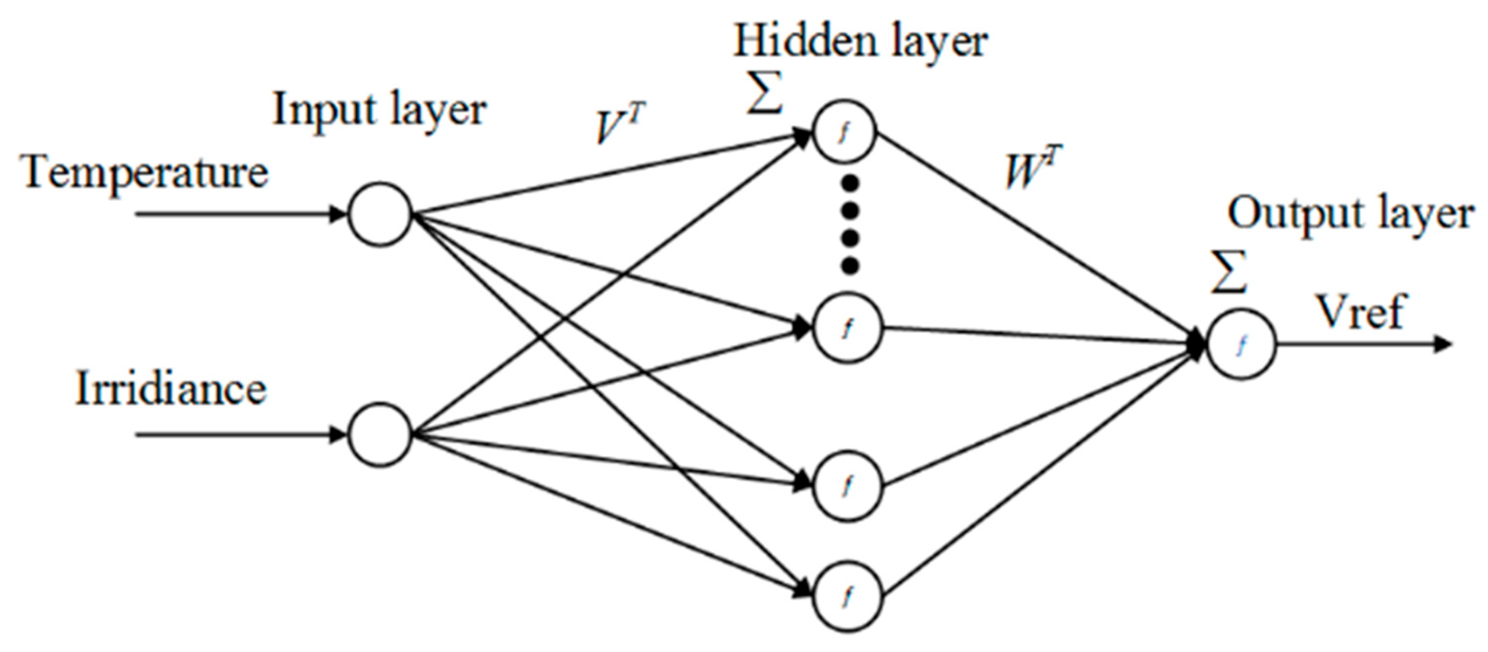
- Generating the reference voltage () trajectory using a pre-calibrated FNN model.
- (2)
- Formulating a well-postulated online adaptation law using the nonlinear Hyperbolic Secant Function (HSF) of the system’s state error and the error derivative variables. The waveform of the HSF is configured using well-established state-error-dependent meta-rules.
- (3)
- Augmenting the FOPID controller with the adaptation law that dynamically self-adjusts the fractional orders of the integral and differential operators to realize the A-FOPID controller that accurately tracks the trajectory.
- (4)
- Verifying the proposed controller’s efficacy by carrying out customized simulations in the MATLAB/Simulink (R2022b) environment that analyze the controller’s behavior under the influence of step changes in the irradiance levels and ambient temperature conditions.
2. System Description
2.1. Photovoltaic System Model
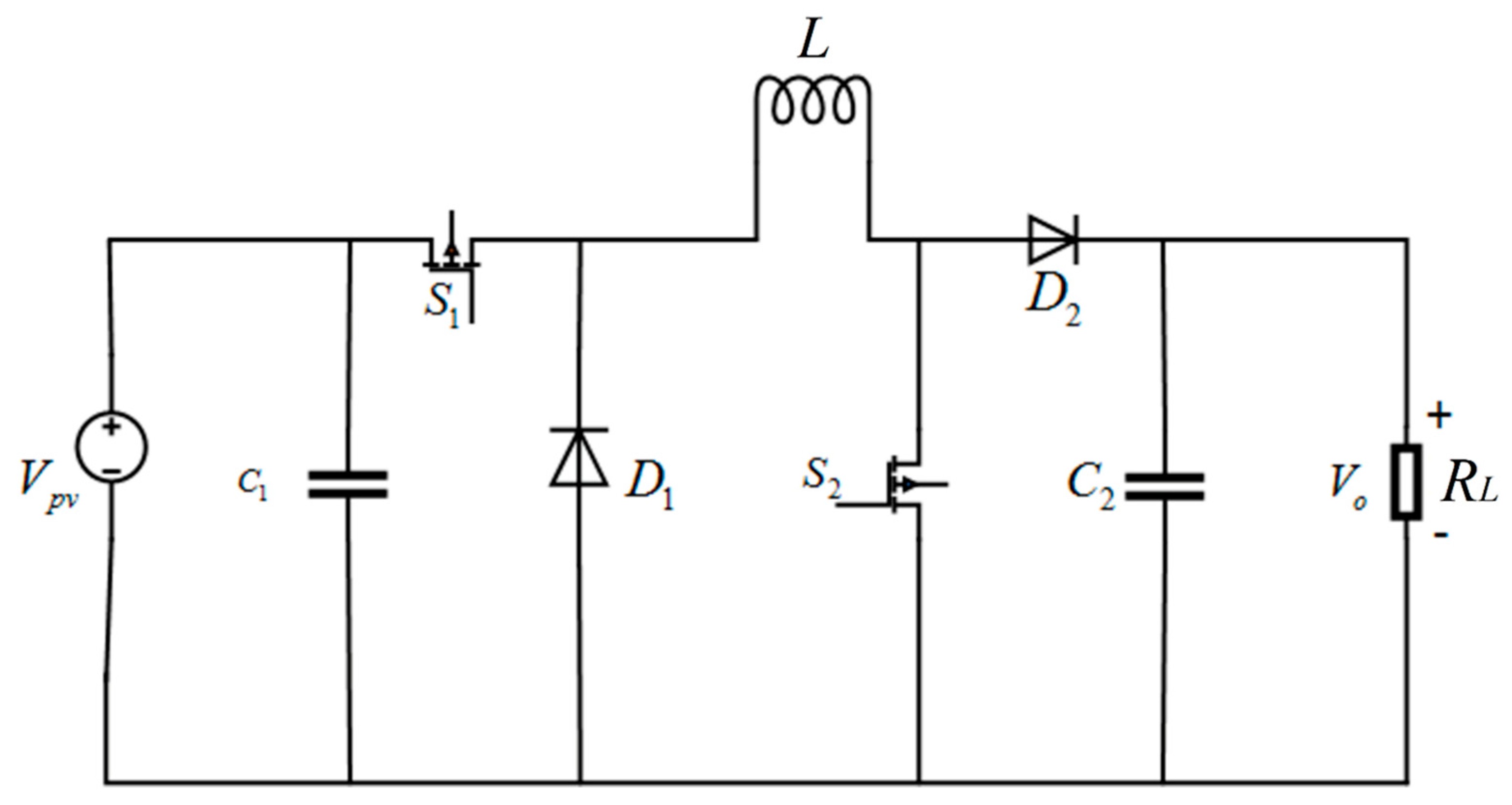
2.2. Buck-Boost Converter Model
2.3. Reference Voltage Generation
2.4. Fractional Order PID Control Law
- The open loop system’s phase at the gain cross-over frequency must satisfy: , where is the phase margin and is the system’s overall transfer function that is derived using (10).
- The open loop system’s gain at must satisfy: .
- To uphold robustness against loop-gain changes, the phase must satisfy: .
- To reject high-frequency noise , the closed-loop transfer function must satisfy: .
- To reject low-frequency noise , the sensitivity function must satisfy: .
3. Proposed Adaptive FOPID Control Scheme
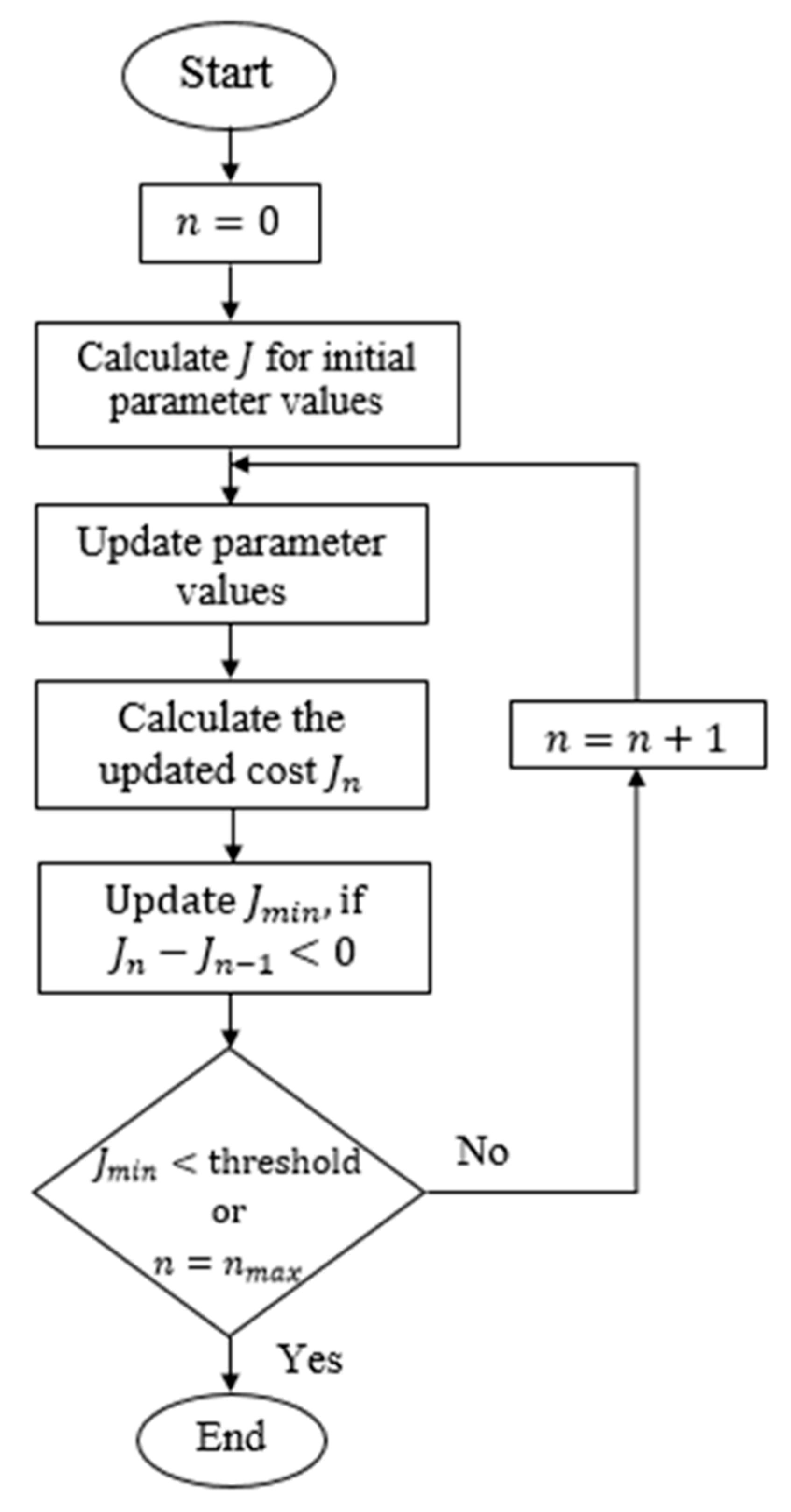
4. Parameter Tuning Procedure
5. Simulation Results and Discussions
5.1. Simulation Setup
5.2. Simulations and Results
- Reference tracking under varying irradiance: This simulation examines the capability of the FOPID and A-FOPID control laws to extract maximum power under varying irradiance levels. In this test case, step changes are introduced in the irradiance levels at regular intervals, as shown in Figure 10, while the temperature is kept constant at 25 °C (298 K). The designed controllers are tasked with tracking the trajectory generated by the FNN scheme for the varying irradiance profiles. The resulting reference voltage trajectory tracking behavior and MPPT profile of the PV array are shown in Figure 11 and Figure 12, respectively. The results show that the A-FOPID achieves the MPP without any significant overshoots and with a faster response speed. It also minimizes the steady-state fluctuations in the response. Whereas the FOPID controller exhibits a relatively slower response speed with persistent oscillations (and chattering) in the response. The results validate the superior robustness and reference tracking accuracy of the A-FOPID controller.
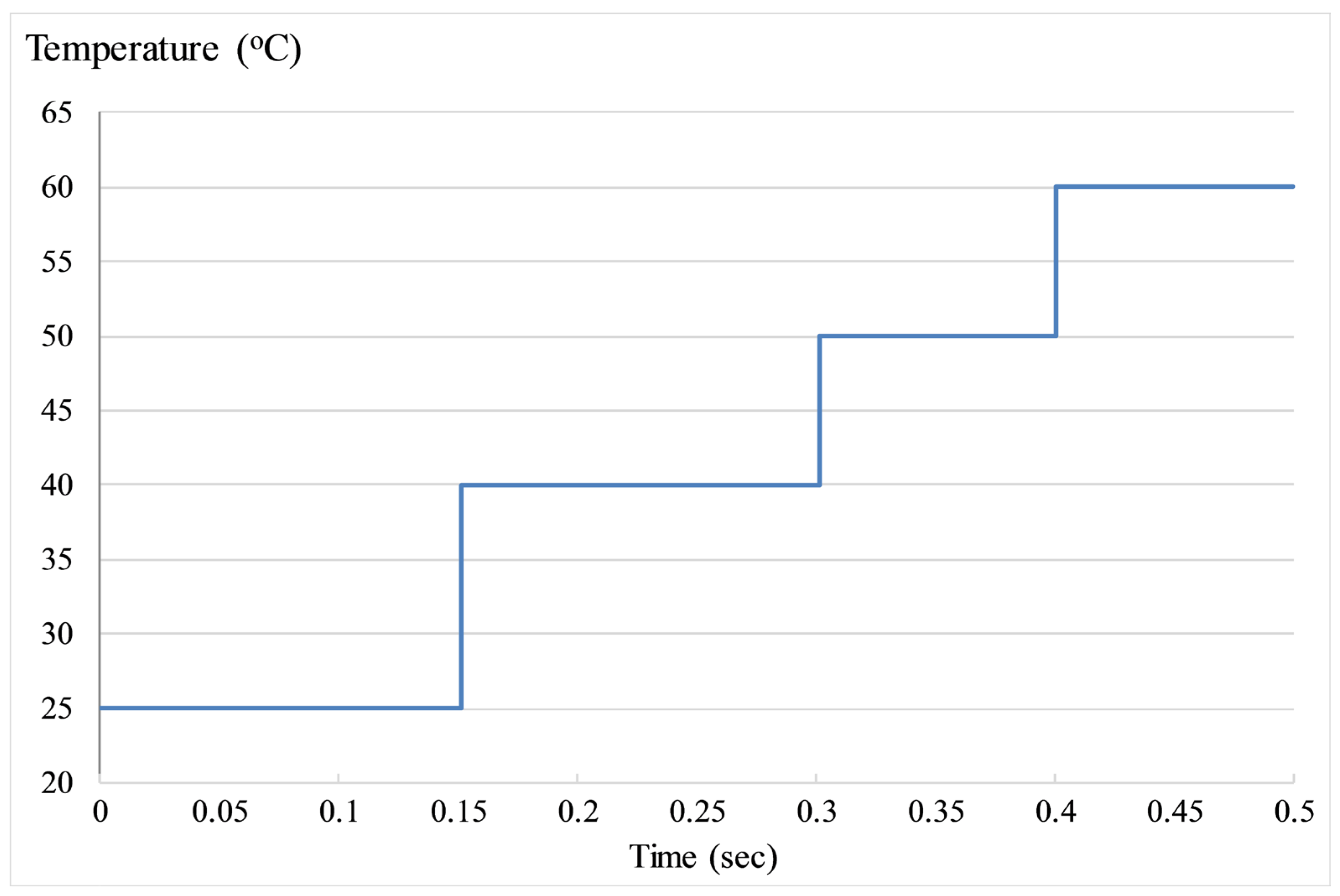
- Reference tracking under varying ambient temperatures: This simulation examines the controller’s ability to extract maximum power under varying outdoor temperature levels. The temperature levels are varied as shown in Figure 13, while the irradiance is kept constant at 1000 W/m2. The controllers track the reference trajectory for the varying temperature profiles. The reference voltage and the MPP tracking profiles are shown in Figure 14 and Figure 15, respectively. The results show that the A-FOPID controller achieves the MPP with better accuracy, a faster response speed, and minimal oscillations. The FOPID controller exhibits a relatively slower response speed with oscillations. The results validate the enhanced reference tracking behavior of the A-FOPID controller.
5.3. Analytical Discussions
- VRMSE: Root-mean-squared value of error, .
- OS: Overshoot in after the initial start-up.
- Tset: Time taken by the signal to settle at the desired voltage after initial start-up.
- PRMSE: Root-mean-squared value of the error in the output power levels of the PV array.
6. Conclusions
Author Contributions
Funding
Data Availability Statement
Conflicts of Interest
References
- Irfan, M.; Iqbal, J.; Iqbal, A.; Iqbal, Z.; Riaz, R.A.; Mehmood, A. Opportunities and challenges in the control of smart grids-Pakistani perspective. Renew. Sustain. Energy Rev. 2017, 71, 652–674. [Google Scholar] [CrossRef]
- Mohamed, M.A.; Eltamaly, A.M.; Alolah, A.L. PSO-based smart grid application for sizing and optimization of hybrid renewable energy systems. PLoS ONE 2016, 11, e0159702. [Google Scholar] [CrossRef] [PubMed] [Green Version]
- Iqbal, J.; Khan, Z.H. The potential role of renewable energy sources in robot’s power system: A case study of Pakistan. Renew. Sustain. Energy Rev. 2017, 75, 106–122. [Google Scholar] [CrossRef]
- Hassan, M.U.; Nawaz, M.I.; Iqbal, J. Towards autonomous cleaning of photovoltaic modules: Design and realization of a robotic cleaner. In Proceedings of the IEEE International Conference on Latest trends in Electrical Engineering & Computing Technologies, Karachi, Pakistan, 15–16 November 2017. [Google Scholar]
- Zhou, S.; Kang, L.; Sun, J.; Guo, G.; Cheng, B.; Cao, B.; Tang, Y. A novel maximum power point tracking algorithms for standalone photovoltaic system. Int. J. Control Autom. Syst. 2011, 8, 1364–1371. [Google Scholar] [CrossRef]
- Pandya, R.; Vardia, M. Grid-connected PV system with MPPT control and P&O technique. Int. J. Adv. Res. Innov. Ideas Educ. 2016, 2, 530–534. [Google Scholar]
- Jena, S.; Sahoo, S.; Panigrahi, C.K. Effect of irradiance onyield factor of solar photovoltaic plant-A case study. In Proceedings of the 2017 International Conference on Innovative Mechanisms for Industry Applications, Bangalore, India, 21–23 February 2017; pp. 597–601. [Google Scholar]
- Razak, A.; Yusoff, M.I.; Zhe, L.W.; Irwanto, M.; Ibrahim, S.; Zhafarina, M. Investigation of the Effect Temperature on Photovoltaic (PV) Panel Output Performance. Int. J. Adv. Sci. Eng. Inf. Technol. 2016, 6, 682–688. [Google Scholar] [CrossRef]
- Anjum, M.B.; Khan, Q.; Ullah, S.; Hafeez, G.; Fida, A.; Iqbal, J.; Albogamy, F.R. Maximum Power Extraction from a Standalone Photo Voltaic System via Neuro-Adaptive Arbitrary Order Sliding Mode Control Strategy with High Gain Differentiation. Appl. Sci. 2022, 12, 2773. [Google Scholar] [CrossRef]
- Hameed, W.I.; Saleh, A.L.; Sawadi, B.A.; Al-Yasir, Y.I.A.; Abd-Alhameed, R.A. Maximum Power Point Tracking for Photovoltaic System by Using Fuzzy Neural Network. Inventions 2019, 4, 33. [Google Scholar] [CrossRef] [Green Version]
- Subudhi, B.; Pradhan, R. A Comparative Study on Maximum Power Point Tracking Techniques for Photovoltaic Power Systems. IEEE Trans. Sustain. Energy 2013, 4, 89–98. [Google Scholar] [CrossRef]
- Bhatnagar, P.; Nema, R. Maximum power point tracking control techniques: State-of-the-art in photovoltaic applications. Renew. Sustain. Energy Rev. 2013, 23, 224–241. [Google Scholar] [CrossRef]
- Kollimalla, S.K.; Mishra, M.K. Variable Perturbation Size Adaptive P&O MPPT Algorithm for Sudden Changes in Irradiance. IEEE Trans. Sustain. Energy 2014, 5, 718–728. [Google Scholar]
- Loukriz, A.; Haddadi, M.; Messalti, S. Simulation and experimental design of a new advanced variable step size Incremental Conductance MPPT algorithm for PV systems. ISA Trans. 2016, 62, 30–38. [Google Scholar] [CrossRef] [PubMed]
- Feroz Mirza, A.; Mansoor, M.; Ling, Q.; Khan, M.I.; Aldossary, O.M. Advanced variable step size incremental conductance MPPT for a standalone PV system utilizing a GA-tuned PID controller. Energies 2020, 13, 4153. [Google Scholar] [CrossRef]
- Uswarman, R.; Munawar, K.; Ramli, M.A.M.; Bouchekara, H.R.E.H.; Hossain, M.A. Maximum Power Point Tracking in Photovoltaic Systems Based on Global Sliding Mode Control with Adaptive Gain Scheduling. Electronics 2023, 12, 1128. [Google Scholar] [CrossRef]
- Haq, I.U.; Khan, Q.; Ullah, S.; Khan, S.A.; Akmeliawati, R.; Khan, M.A.; Iqbal, J. Neural network-based adaptive global sliding mode MPPT controller design for stand-alone photovoltaic systems. PLoS ONE 2022, 17, e0260480. [Google Scholar] [CrossRef]
- Kharb, R.K.; Shimi, S.; Chatterji, S.; Ansari, M.F. Modeling of solar PV module and maximum power point tracking using ANFIS. Renew. Sustain. Energy Rev. 2014, 33, 602–612. [Google Scholar] [CrossRef]
- Ali, K.; Khan, L.; Khan, Q.; Ullah, S.; Ahmad, S.; Mumtaz, S.; Karam, F.W.; Naghmash. Robust Integral Backstepping Based Nonlinear MPPT Control for a PV System. Energies 2019, 12, 3180. [Google Scholar] [CrossRef] [Green Version]
- Saleem, O.; Abbas, F.; Iqbal, J. Complex fractional-order LQIR for inverted-pendulum-type robotic mechanisms—Design and experimental validation. Mathematics 2023, 11, 913. [Google Scholar] [CrossRef]
- Saleem, O.; Shami, U.T.; Mahmood-ul-Hasan, K. Time-optimal control of DC-DC buck converter using single-input fuzzy augmented fractional-order PI controller. Int. Trans. Elect. Energy Syst. 2019, 29, e12064. [Google Scholar] [CrossRef]
- Saleem, O.; Rizwan, M.; Khizar, A.; Ahmad, M. Augmentation of fractional-order PI controller with nonlinear error-modulator for enhancing robustness of DC-DC boost converters. J. Pow. Electron. 2019, 19, 835–845. [Google Scholar]
- Jeba, P.; Immanuel Selvakumar, A. FOPID based MPPT for photovoltaic system. Energy Sour. Part A Recover. Util. Environ. Eff. 2018, 40, 1591–1603. [Google Scholar] [CrossRef]
- Nasir, A.; Rasool, I.; Sibtain, D.; Kamran, R. Adaptive Fractional Order PID Controller Based MPPT for PV Connected Grid System Under Changing Weather Conditions. J. Elect. Eng. Technol. 2021, 16, 2599–2610. [Google Scholar] [CrossRef]
- Bouakkaz, M.S.; Boukadoum, A.; Boudebbouz, O.; Fergani, N.; Boutasseta, N.; Attoui, I.; Bouraiou, A.; Necaibia, A. Dynamic performance evaluation and improvement of PV energy generation systems using Moth Flame Optimization with combined fractional order PID and sliding mode controller. Sol. Energy 2020, 199, 411–424. [Google Scholar] [CrossRef]
- Rawat, A.; Jha, S.K.; Kumar, B.; Mohan, V. Nonlinear fractional order PID controller for tracking maximum power in photo-voltaic system. J. Intell. Fuzzy Syst. 2020, 38, 6703–6713. [Google Scholar] [CrossRef]
- Saleem, O.; Awan, F.G.; Mahmood-ul-Hasan, K.; Ahmad, M. Self-adaptive fractional-order LQ-PID voltage controller for robust disturbance compensation in DC-DC buck converters. Int. J. Numer. Model. 2020, 33, e2718. [Google Scholar] [CrossRef]
- Bellia, H.; Youcef, R.; Fatima, M. A detailed modeling of photovoltaic module using MATLAB. NRIAG J. Astron. Geophys. 2014, 3, 53–61. [Google Scholar] [CrossRef] [Green Version]
- Omar, M.A.; Mahmoud, M. Design and simulation of DC/DC boost converter with maximum power point tracking for grid connected PV inverter considering the nonlinearity of the PV generator. Int. J. Energy Convers. 2019, 7, 241–252. [Google Scholar] [CrossRef]
- Gaboriault, M.; Notman, A. A high efficiency, non-inverting, buck-boost DC-DC converter. In Proceedings of the Annual IEEE Applied Power Electronics Conference and Exposition, Anaheim, CA, USA, 22–26 February 2004; pp. 1411–1415. [Google Scholar]
- Hagan, M.T.; Demuth, H.B.; Beale, M.H.; Jesus, O.D. Neural Network Design; PWS Publishing Co.: Boston, MA, USA, 1996; Volume 20. [Google Scholar]
- Li, Z.; Liu, L.; Dehgan, S.; Chen, Y.Q.; Xue, D. A review and evaluation of numerical tools for fractional calculus and fractional order controls. Int. J. Control. 2017, 90, 1165–1181. [Google Scholar] [CrossRef] [Green Version]
- Hui, P.; Ping, W.; Weihua, L. Model based fractional order pid controller design and simulation of pressure swing adsorption. In Proceedings of the 38th Chinese Control Conference (CCC), Guangzhou, China, 27–30 July 2019; pp. 2880–2883. [Google Scholar]
- Saleem, O.; Mahmood-Ul-Hasan, K. Adaptive collaborative speed control of PMDC motor using hyperbolic secant functions and particle swarm optimization. Turkish J. Electr. Eng. Comput. Sci. 2018, 26, 1612–1622. [Google Scholar]
- Saleem, O.; Rizwan, M. Performance optimization of LQR-based PID controller for DC-DC buck converter via iterative-learning-tuning of state-weighting matrix. Int. J. Numer. Model. 2019, 32, e2572. [Google Scholar] [CrossRef]
- Kondawar, S.S.; Vaidya, U.B. A Comparison of two MPPT techniques for PV system in Matlab/Simulink. Int. J. Eng. Res. Dev. 2012, 2, 73–79. [Google Scholar]
- Daraban, S.; Petreus, D.; Morel, C. A novel MPPT (maximum power point tracking) algorithm based on a modified genetic algorithm specialized on tracking the global maximum power point in photovoltaic systems affected by partial shading. Energy 2014, 74, 374–388. [Google Scholar] [CrossRef]
- Yang, B.; Zhu, T.; Wang, J.; Shu, H.; Yu, T.; Zhang, X.; Yao, W.; Sun, L. Comprehensive overview of maximum power point tracking algorithms of PV systems under partial shading condition. J. Clean. Prod. 2020, 268, 121983. [Google Scholar] [CrossRef]


| Parameter | Value | Units |
|---|---|---|
| 17.56 | ||
| A/°C | ||
| 1.8 | - | |
| 72 | - | |
| 1 | - | |
| Open circuit voltage | 165.8 | |
| Maximum power | 1555 | |
| Voltage at MPP | 102.6 | |
| Current at MPP | 15.16 |
| Parameter | Value | Units |
|---|---|---|
| Controller | ||
|---|---|---|
| 0 | 0 | P |
| 0 | 1 | PD |
| 1 | 0 | PI |
| 1 | 1 | PID |
| Parameters | Selection Range | Initial Value | Optimized Values | |
|---|---|---|---|---|
| FOPID | A-FOPID | |||
| [0, 0.1] | 1 × 10⁻² | 0.432 | 0.427 | |
| [0, 0.1] | 1 × 10⁻² | 0.106 | 0.112 | |
| [0, 0.1] | 1 × 10⁻² | 0.028 | 0.034 | |
| [0, 1] | 0.1 | 0.84 | - | |
| [0, 1] | 0.1 | 0.66 | - | |
| [0, 1] | 0.01 | - | 0.095 | |
| [0, 1] | 0.01 | - | 0.028 | |
| Simulation | Performance Indicator | Controller | Performance Improvement | ||
|---|---|---|---|---|---|
| Metric | Unit | FOPID | A-FOPID | ||
| A | VRMSE | V | 35.05 | 27.28 | 22.2% |
| OS | V | 25.35 | 3.38 | 86.7% | |
| Tset | sec | 0.014 | 0.012 | 14.3% | |
| PRMSE | kW | 5.15 | 3.21 | 37.7% | |
| B | VRMSE | V | 27.50 | 19.63 | 28.6% |
| OS | V | 30.61 | 4.88 | 84.0% | |
| Tset | sec | 0.012 | 0.011 | 8.3% | |
| PRMSE | kW | 1.77 | 0.92 | 48.0% | |
Disclaimer/Publisher’s Note: The statements, opinions and data contained in all publications are solely those of the individual author(s) and contributor(s) and not of MDPI and/or the editor(s). MDPI and/or the editor(s) disclaim responsibility for any injury to people or property resulting from any ideas, methods, instructions or products referred to in the content. |
© 2023 by the authors. Licensee MDPI, Basel, Switzerland. This article is an open access article distributed under the terms and conditions of the Creative Commons Attribution (CC BY) license (https://creativecommons.org/licenses/by/4.0/).
Share and Cite
Saleem, O.; Ali, S.; Iqbal, J. Robust MPPT Control of Stand-Alone Photovoltaic Systems via Adaptive Self-Adjusting Fractional Order PID Controller. Energies 2023, 16, 5039. https://doi.org/10.3390/en16135039
Saleem O, Ali S, Iqbal J. Robust MPPT Control of Stand-Alone Photovoltaic Systems via Adaptive Self-Adjusting Fractional Order PID Controller. Energies. 2023; 16(13):5039. https://doi.org/10.3390/en16135039
Chicago/Turabian StyleSaleem, Omer, Shehryaar Ali, and Jamshed Iqbal. 2023. "Robust MPPT Control of Stand-Alone Photovoltaic Systems via Adaptive Self-Adjusting Fractional Order PID Controller" Energies 16, no. 13: 5039. https://doi.org/10.3390/en16135039