Validation of the Eulerian–Eulerian Two-Fluid Method and the RPI Wall Partitioning Model Predictions in OpenFOAM with Respect to the Flow Boiling Characteristics within Conventional Tubes and Micro-Channels

Abstract

Flow boiling within conventional, mini and micro-scale channels is encountered in a wide range of engineering applications such as nuclear reactors, steam engines and cooling of electronic devices. Due to the high complexity and importance of the boiling process, several numerical and experimental investigations have been conducted for the better understanding of the underpinned physics and heat transfer characteristics. One of the most widely used numerical approaches that can analyse such phenomena is the Eulerian–Eulerian two-fluid method in conjunction with the RPI model. However, according to the current state-of-the-art methods this modelling approach heavily relies on empirical closure relationships derived for conventional channels, limiting its applicability to mini- and micro-scale channels. The present paper aims to give further insights into the applicability of this modelling approach for non-conventional channels. For this purpose, a numerical investigation utilising the Eulerian–Eulerian two-fluid model and the RPI wall heat flux partitioning model in OpenFOAM 8.0 is conducted. Initially the parameters comprising the empirical closure relationships used in the RPI sub-models are tuned against the DEBORA experiments on conventional channels, through an extensive sensitivity analysis. In the second part of the investigation, numerical simulations against flow boiling experiments within micro-channels are performed, utilising the previously optimised and validated model setup. Furthermore the importance of including a bubble coalescence and break-up sub-model to capture parameters such as the radial velocity profiles, is also illustrated. However, when the optimal model setup, in conventional tubes, is used against micro-channel experiments, the need to develop new correlations from data obtained from mini and micro-scale channel studies, not from experimental data on conventional channels, is revealed.

1. Introduction

Due to the involvement of transported latent heat, boiling is recognised as one of the most effective modes of heat transfer, receiving considerable attention from many researchers both in industry and academia. In particular, sub-cooled flow boiling is used in several industrial applications where effective cooling is required such as nuclear refrigeration, the aerospace industry and microelectronic cooling devices [1]. This boiling process is very complicated and difficult to analysed due to bubble nucleation, growth, departure and their non-uniform dispersion close to the heated wall as well as the heat, mass and momentum exchange within the developed two-phase flows (liquid and vapour) [2,3]. The complicated nature of such transient phenomena has made understanding the underpinning physical mechanisms of the boiling process within channels a very challenging task. So far, many experimental works have focused on developing empirical correlations based on a high number of experimental data using conventional channels with various geometrical characteristics and a wide range of working fluids, materials and operating conditions. These empirical correlations are either subsequently utilised by other researchers to confirm the accuracy of their measurements or they are used in numerical models as sub-models to predict important flow boiling characteristics usually measured on the radial axis (e.g., radial profiles) in the axial direction (e.g., axial profiles) [4,5,6,7]. To numerically predict flow boiling characteristics, it is necessary that an appropriate CFD modelling approach is employed by selecting suitable boiling sub-models. One of the most widely used CFD approaches that can analyse such phenomena is the Eulerian–Eulerian two-fluid method [8,9]. This method treats each phase separately with its own set of governing equations for the conservation of mass, momentum and energy. These conservation equations are usually coupled with empirical closures for the momentum and mass exchange between the liquid and vapour phases, as well as for physical mechanisms such as the heat and mass forces across the interface, thus determining the level of thermal and hydraulic non-equilibrium between the phases [10]. The closures that relate to the boiling heat transfer constitute part of the wall heat flux partitioning model, where the partitioning of the wall heat flux into these physical mechanisms is responsible for the wall boiling heat transfer, are described. So far, various models have been developed for the prediction of heat transfer and wall heat flux partitioning [11,12,13]. A widely used wall partitioning model in boiling phenomena within the two-fluid numerical framework is the RPI (Rensselaer Polytechnic Institute) model proposed and developed by Kurul and Podowski [14]. It is based on the principle that all wall heat energy from the wall is transformed into the fluid in the near-wall region, divided into three different components: a single-phase convective heat flux, an evaporative heat flux, and a wall quenching heat flux [15]. This model has been implemented in various commercial/in-house codes and has been validated against various experiments by many researchers, concluding that the closures included in the model are highly problem-specific and their range of validity needs to be carefully considered [16]. Therefore, many numerical investigations into the RPI model have been performed, trying to find the appropriate sub-models for important wall boiling parameters, such as the nucleation site density ($N_w$), bubble departure diameter ($D_w$) and bubble departure frequency (f), in particularly trying to select suitable values for their empirical constants, so that they can be widely applied in industry and academia, at various conditions, avoiding continuous modifications/alterations to the model. In more detail, Tu and Yeoh [17] validated the different correlations for the $N_w$, $D_w$ and f, using the commercial CFD toolbox of CFX-4.2 on the sub-cooled flow boiling of circular tubes with a $12.7$ $\mathrm{m}$$\mathrm{m}$ inner diameter, under low-pressure conditions. It was shown that the models developed for higher pressures may not be suitable for low-pressure predictions without adequate modifications. Koncar et al. [18] performed numerical investigations on circular tubes with 19.05 and $18.95$ $\mathrm{m}$$\mathrm{m}$ inner diameter, on the same group of closure models for the $N_w$, $D_w$ and f on sub-cooloed flow boiling at low pressures (<$0.13$ $\mathrm{M}$$\mathrm{Pa}$) using CFX-4.3. They obtained results with good overall agreement compared to the experimental data. Drzewiecki et al. [19] conducted a sensitivity investigation into the empirical parameters of the boiling two-fluid model in conjunction with the RPI model against the DEBORA experiments, finding that the wall superheat and void fraction were the most sensitive to the evaporative heat flux and bubble detachment diameter.

Krepper et al. [20] performed numerical simulations to validate and identify potential weak points of the RPI model for sub-cooled boiling conditions in a circular tube with an inner diameter of $15.4$ $\mathrm{m}$$\mathrm{m}$ at various pressure ranges (1.5 to 15 $\mathrm{M}$$\mathrm{Pa}$), mass flow rates (400 to 2000 kg m⁻² s⁻¹) and heat flux conditions, based on experiments performed by Bartolomej et al. [21,22]. They proved that the RPI wall boiling model was able to compute the cross-sectional-averaged vapour volume fraction in perpendicular heated pipes with good accuracy compared to the corresponding experiments, and the position at which nucleate boiling bubble departure occurred was predicted as well. In two other numerical studies performed by Krepper et al. [23,24], where the DEBORA experiments were reproduced using the commercial software CFX, on sub-cooled flow boiling conditions with tubes of inner diameter $19.2$ $\mathrm{m}$$\mathrm{m}$ with various pressures (1.46 to $2.62$ $\mathrm{M}$$\mathrm{Pa}$) and inlet temperature ranges (304.31 to $343.30$ $\mathrm{K}$), the numerical results of the regional flow characteristics measured in the radial and axial directions were analysed and discussed, including the local distribution of the void fraction, the temperature of the liquid, and the axial liquid and vapour velocity. The results clearly showed that the active nucleation site density has high impact on the wall superheat, but has minimal impact on the gas volume fraction and negligible influence on the temperature of the liquid. In more detail, in [23] it was found that tuning of the empirical coefficient in $D_w$ had a major influence on the resulting volume fraction, thus impacting the quenching heat flux which was an order of magnitude lower compared to the evaporation heat flux. In their second study [24], a different method of calculating the bubble detachment diameter was developed by coupling a population balance model with the two-fluid model. This approach made the model rely less on the user inputs, added more empirical terms for the bubble coalescence and break-up, which in turn needed to be correctly modelled. In this method, the bubble coalescence away from the heated wall was able to be captured; however, the predictions of the volume fraction were found to be less sensitive to the size of the bubbles far from the wall. Recently, the RPI model was also used by Gu et al. [25] to conduct a CFD study on Fluent (v15.0) based on the sub-cooled flow boiling experiments of Bartolomej et al. [21,22], examining different closure models to achieve the most accurate solution compared to the corresponding experiments. They concluded that the nucleation site density and bubble diameter significantly impact various key heat transfer parameters (e.g., volume fraction, liquid temperature), proposing that the best closure model is a combination of the empirical correlation of Lemmert and Chawla [26] for the nucleation site density, Unal [27] for the bubble detachment diameter, and Cole [28] for the bubble departure frequency. More recently, different numerical studies using the Eulerian–Eulerian two-fluid model for the prediction of various parameters have verified the use of different empirical model combinations of the wall partitioning model, depending on the working conditions [29,30,31,32]; however, they did not conclude a more global combination of the models that could be widely used. At this point it is also worth mentioning that the interfacial dynamics in the boiling heat transfer phenomena can also be modelled numerically with other techniques such as interface capturing methods (i.e., [33]) and mesh-less techniques such as the moving particle semi-implicit method (i.e., [34]); however, such techniques mainly focus on resolving the interface dynamics and are thus more applicable to studying local phenomena. Hence, such techniques are not reviewed in the present manuscript as we focus on more global CFD methods such as the Eulerian–Eulerian two-fluid approach.

From the above review it is evident that the Eulerian–Eulerian two-fluid model and its RPI model, on the basis of wall heat flux partitioning, constitutes a promising combination to provide important answers and valuable information on key heat transfer characteristics of flow boiling, not only in conventional tubes but in more advanced cooling methods, with modifications, such as flow boiling within mini- and micro-channels. However, the constitutive empirical relations that are based on limited data or under specific operational conditions, together with the requirement for the prescription of correct sub-models, remain the main limitation of this approach. In the present paper the two-fluid model and the RPI wall heat flux partitioning model within the open-source CFD package OpenFOAM, are employed in order to numerically reproduce the benchmark experimental test cases of DEBORA [35,36]. Precisely, two different investigations are conducted. Initially, in order for the numerical simulations to show good agreement with the experimental results, tuning of the empirical parameters comprising the closures is performed. Conducting such research shows that OpenFOAM is able to predict important heat transfer characteristics with a good degree of accuracy compared to previous investigations with commercial CFD codes. In the second stage of the present paper, the reproduction of experimental work available in the literature on flow boiling within micro-channels is performed, utilising the optimised “tuned” model parameters from the validation against the conventional DEBORA cases, indicating the need to develop new correlations based on data obtained from mini- and micro-scale channel studies, not experimental data in conventional tubes.

2. Numerical Simulation Framework

2.1. Two-Fluid Model

The simulations presented in this study have been performed using the open-source CFD toolbox of OpenFOAM V. 8.0. Particularly the diabatic Eulerian–Eulerian two-fluid solver multiPhaseEulerFoam is used in the present work to consideration the thermodynamic non-equilibrium between the liquid and vapour phases. In this model both phases are treated as interpenetrating continua with conservation equations for mass, momentum and energy formulated for each phase (e.g., liquid and vapour) and weighted by the so-called volume fraction which specifies the fractions of the average volume occupied by each phase and as continuous functions of space and time [8,9].

The continuity equation of the two-fluid model can be written as

$$\frac{\partial {\alpha }_k{\rho }_k}{\partial t}+\nabla ·\left({\alpha }_k{\rho }_k{\mathbf{U}}_k\right)={\dot{m}}_{kj}-{\dot{m}}_{jk}$$

(1)

where ${\dot{m}}_{kj}$ and ${\dot{m}}_{jk}$ is the mass transfer rate between the jth and kth phases, respectively.

The momentum equation for the liquid and vapour phases are as follows

$$\begin{array}{c}\hfill \frac{\partial {\alpha }_k{\rho }_k{\mathbf{U}}_k}{\partial t}+\nabla ·\left({\alpha }_k{\rho }_k{\mathbf{U}}_k{\mathbf{U}}_k\right)=-{\alpha }_k\nabla p_k+\nabla ·\left[{\alpha }_k({\overline{\overline{\tau }}}_k+{\overline{\overline{\tau }}}_k^{Re})\right]+{\alpha }_k{\rho }_k\mathbf{g}+{\mathbf{M}}_{ki}\end{array}$$

(2)

where ${\alpha }_k$, ${\rho }_k$ and ${\mathbf{U}}_k$ are the volume fraction, density and velocity vector for each phase k, respectively. The terms $\overline{\overline{\tau }}$${}_k$ and $\overline{\overline{\tau }}$${}_k^{Re}$ are the viscous and Reynolds (turbulent) stresses, respectively. Additionally, ${\mathbf{M}}_{ki}$ is the averaged inter-phase momentum transfer term.

The Reynolds and viscous stress tensors are modelled using Boussinesq’s hypothesis using the Newtonian strain–stress relation, given by

$${\overline{\overline{\tau }}}_k+{\overline{\overline{\tau }}}_k^{Re}=-({\mu }_k+{\mu }_k^t)(\nabla {\mathbf{U}}_k+\nabla {\mathbf{U}}_k^T-\frac{2}{3}I\nabla \times {\mathbf{U}}_k)+\frac{2}{3}I{k}_k,$$

(3)

where I, ${\mu }_k$, ${\mu }_k^t$ and $k_k$ are the identity tensor, physical dynamic viscosity, turbulent dynamic viscosity and turbulent kinetic energy of phase k, respectively.

To describe the conservation of energy in Eulerian multiphase applications, a separate enthalpy equation can be written for each phase:

$$\begin{array}{c}\hfill \frac{\partial \left({\alpha }_k{\rho }_k{H}_k\right)}{\partial t}+\nabla ·\left({\alpha }_k{\rho }_k{\mathbf{U}}_k{H}_k\right)=\nabla ·({\alpha }_k{\lambda }_k\nabla T_k)+\nabla ·({\alpha }_k\frac{{\mu }_{T,k}}{P{r}_{T,k}}\nabla H_k)\\ \hfill +\sum _{l=1}^2({\dot{m}}_{jk}{H}_j-{\dot{m}}_{kj}{H}_k)+Q_{H,int}\end{array}$$

(4)

where $H_j$ and $H_k$ is the enthalpy of the jth and kth phases, respectively, ${\lambda }_k$ is the thermal conductivity of phase k, ${\dot{m}}_{lk}$ and ${\dot{m}}_{kl}$ is the mass transfer rate from the liquid phase to the vapour phase, respectively, $P{r}_{T,k}$ is turbulent Prandtl number, $Q_{H,int}$ is the heat flux exchanged by the interface between the two phases, and the terms inside the summation represent the total enthalpy exchanged in the phase change.

2.2. Turbulence Model

For the continuous liquid phase, the turbulent fluctuations are modelled by a shear-stress turbulence (SST) $\kappa -\omega$ model (KOmegaSSTSato) introduced by Sato et al. [37] and Menter et al. [38]. The SST model works by solving a turbulence/frequency-based model $\kappa -\omega$ near the wall and a $\kappa -ϵ$ model in the bulk flow. The $\kappa -ϵ$ turbulence model (continuousGasKEpsilon) is used for the dispersed gas phase. This particular turbulence model is used for the vapour phase in a multiphase system as a permanent numerical framework that supports phase inversion. Precisely, in this turbulence model when the fraction of the vapour phase approaches 0, a contribution from the liquid phase is blended into the turbulence equations. This results in the model being reverted in a pure single-phase form.

2.3. Interfacial Momentum Transfer

From the momentum Equation (2) it is clear that the interfacial momentum term cannot be ignored as it plays a significant role in determining the overall flow dynamics. In particular, the interfacial momentum transfer is caused by the forces acting between the two phases such as the forces acting on the rising bubbles from the liquid which surrounds it, and are a function of four established interfacial momentum transfer mechanisms. These include the drag force ${\mathbf{M}}_{\mathbf{ki}}^{\mathbf{D}}$, the lift force ${\mathbf{M}}_{\mathbf{ki}}^{\mathbf{L}}$, the wall lubrication force ${\mathbf{M}}_{\mathbf{ki}}^{\mathbf{WL}}$, the turbulent dispersion force ${\mathbf{M}}_{\mathbf{ki}}^{\mathbf{TD}}$ and the virtual mass force ${\mathbf{M}}_{\mathbf{ki}}^{\mathbf{VM}}$. Hence, the interfacial momentum exchange is the summary of these forces:

$${\mathbf{M}}_{\mathbf{ki}}={\mathbf{M}}_{\mathbf{ki}}^{\mathbf{D}}+{\mathbf{M}}_{\mathbf{ki}}^{\mathbf{L}}+{\mathbf{M}}_{\mathbf{ki}}^{\mathbf{WL}}+{\mathbf{M}}_{\mathbf{ki}}^{\mathbf{TD}}$$

(5)

The virtual mass force becomes dominant when there are density differences within the flow; however, in the present study this term is neglected where the steady state of flow is concerned [39,40].

2.3.1. Drag Force

The drag force represents the force acting on the rising bubbles by the fluid, depending on both the size and shape. The drag model describes how the drag affects the phases that they impart on one another. In the present work, the Ishii–Zuber correlation is chosen, expressed as:

$${\mathbf{M}}_{\mathbf{ki}}^{\mathbf{D}}=-\frac{3}{4}\frac{C_D}{d_B}{\rho }_l{\alpha }_g\left|{\mathbf{U}}_{\mathbf{g}}-{\mathbf{U}}_{\mathbf{l}}\right|({\mathbf{U}}_{\mathbf{g}}-{\mathbf{U}}_{\mathbf{l}})$$

(6)

where $d_B$ is the bubble diameter, ${\rho }_l$ is the density of the liquid phase, and $C_D$ is the drag coefficient, given by

$$C_D=max(min(C_{D,ellipse},C_{D,cap}),C_{D,sphere})$$

(7)

where

$$\begin{array}{cc}\hfill C_{D,sphere}& =max\left(\frac{24}{R{e}_b}(1+0.15R{e}_b^{0.687}),0.44\right)\hfill \\ \hfill C_{D,ellipse}& =\frac{2}{3}E{o}_d^{(1/2)}\hfill \\ \hfill C_{D,cap}& =\frac{8}{3}\hfill \end{array}$$

(8)

the above equation is valid for a bubble Reynolds number $R{e}_b$ > 1000, where

$$R{e}_b=\frac{{\rho }_l\left|\left|{\mathbf{U}}_g-{\mathbf{U}}_l\right|\right|d_B}{{\mu }_m}$$

(9)

with ${\mu }_m$ being the mixture viscosity. $E{o}_d$ is the dimensionless Eötvös number which considers the bubble shape in the drag correlations and is computed as follows:

$$E{o}_d=\frac{g({\rho }_l-{\rho }_g)D_d^2}{\sigma }$$

(10)

where g is the gravitational force, $\sigma$ is the surface tension, and $D_d$ is the maximum bubble horizontal dimension.

2.3.2. Lift Force

For gas–liquid flows, non-drag forces have a huge influence on the flow characteristics, especially in dispersed flows. The lift force plays an important role and greatly impacts the radial distribution of bubbles. According to Drew and Lahey [41], the lift force has a general formulation:

$${\mathbf{M}}_{\mathbf{ki}}^{\mathbf{L}}=-C_L{\alpha }_d{\rho }_c({\mathbf{U}}_g-{\mathbf{U}}_l)\times (\nabla \times {\mathbf{U}}_l)$$

(11)

where $C_L$ is the lift force coefficient, ${\alpha }_d$ is the dispersed phase fraction, ${\rho }_c$ is the continuous phase density, ${\mathbf{U}}_g$ and ${\mathbf{U}}_l$ as the continuous and disperse phase velocities, respectively, and the symbol “×” as the curl product.

Models have been developed based on the empirical correlations to calculate the lift force coefficient $C_L$. In the present study, the model of [42] was adopted. The principal characteristic of this model is that the sign of the lift force can change when the bubbles are substantially non-spherical [43]. The model is defined on the basis of the Eötvös number as:

$$C_L=\left\{\begin{array}{cc}min[0.288tanh(0.121R{e}_b),f\left(E{o}_d\right)]\hfill & \mathrm{if}E{o}_d<4\hfill \\ f\left(E{o}_d\right)=0.00105E{o}_d^3-0.0159E{o}_d^2-0.0204E{o}_d+0.474\hfill & \mathrm{if}4\le E{o}_d\le 10\hfill \\ -0.288\hfill & \mathrm{if}E{o}_d>10\hfill \end{array}\right.$$

where the function $f\left(E{o}_d\right)$ is defined by:

$$f\left(E{o}_d\right)=0.00105E{o}_d^3-0.0159E{o}_d^2-0.0204E{o}_d+0.474$$

(12)

2.3.3. Wall Lubrication Force Model

This force constitutes another lateral force due to surface tension, and prevents the bubbles from attaching to the solid wall. In simulations, this leads to a low gas-phase fraction close to the wall. This force can be generally expressed, according to Antal et al. [44] model adopted in this present model, as:

$$\begin{array}{c}\hfill {\mathbf{F}}_{wl,d}=\frac{{\alpha }_d{\rho }_c\left[({\mathbf{U}}_d-{\mathbf{U}}_c)-(({\mathbf{U}}_d-{\mathbf{U}}_c)·{\mathbf{n}}_w){\mathbf{n}}_w\right]}{D_s}\\ \hfill \times \left(C_{w1}+C_{w2}\frac{D_s}{y_w}\right){\mathbf{n}}_w\end{array}$$

(13)

where ${\mathbf{n}}_w$ represents the wall normal vector, $D_S$ is the Sauter diameter, $y_w$ is the distance from the wall and $C_{w1}=-0.01$ and $C_{w2}=0.05$ are two constants whose values were determined through experiments on a sphere and have been used in the present work.

2.3.4. Turbulent Dispersion Force Model

The turbulent dispersion force considers the effect of the dispersion of bubbles in the turbulent liquid flow. In this study the model developed by Lopez de Bertodano [45] was used,

$${\mathbf{M}}_{\mathbf{ki}}^{\mathbf{TD}}=C_{TD}{\rho }_{b}k{e}_b\nabla {\alpha }_g$$

(14)

where $C_{TD}$ is a modifiable constant set as 1.0 by default, and $k{e}_b$ is the turbulent kinetic energy.

2.4. Boiling Model

For the boiling process to occur, the heated wall temperature needs to exceed the saturation temperature of the working liquid. In numerical models, the bubble generation rate is determined by the wall heat flux partitioning model. In the past, various mechanistic wall heat flux partitioning models have been developed for the prediction of the boiling heat transfer [14,46]. In the present model, the so called RPI model, proposed by Kurul and Podowski [14], is utilised. The key novelty of this wall boiling model is that it divides the total wall heat flux into several components, as shown in Equation (15),

$$q_w=q_q+q_e+q_c$$

(15)

where $q_w$ is the total wall heat flux, $q_q$ represents the quenching heat flux, $q_e$ is the evaporation heat flux and $q_c$ is the heat flux transferred to the liquid by turbulent convection.

The quenching heat flux $q_q$ is the heat flux exchanged due to liquid filling the area close to the after bubble detachment, and can be calculated as follows:

$$q_q=C_{wt}\frac{2k_l}{\sqrt{\pi {\lambda }_l}}\sqrt{f}(T_w-T_l)$$

(16)

where $C_{wt}$ is the bubble waiting time coefficient, $k_l$ is the liquid conductivity, ${\lambda }_l=k_l/\left({\rho }_l{c}_{p,l}\right)$ is the liquid thermal diffusivity, f is the bubble detachment frequency and $T_w$ is the wall temperature.

The evaporative heat flux $q_e$ is calculated as the latent heat carried away by the bubbles departing from the wall, given by

$$q_e=V_d{N}_w{\rho }_g{h}_{fg}f$$

(17)

where $V_d$ is the bubble departure volume, $N_w$ is the nucleation site density, $h_{fg}$ is the latent heat of evaporation and f is the detachment frequency. The last term $q_c$ concerns the single-phase convective heat flux and can be expressed as:

$$q_c=h_c(T_w-T_l)(1-A_b)$$

(18)

where $h_c$ is the single-phase convection heat transfer coefficient and $A_b$ is the bubble influence area coefficient. The coefficient $A_b$ can be computed as:

$$A_b=min\left(1,K\frac{N_w\pi D_w^2}{4}\right)$$

(19)

where the coefficient K, according to Del Valle and Kenning [47], can be calculated from the following relationship,

$$K=4.8e^{\left(-\frac{J_{\mathrm{sub}}}{80}\right)}$$

(20)

where $J_{sub}$ is the sub-cooled Jacob number.

2.4.1. Closure Relations

As shown in the above wall heat flux equations, the accurate modelling of the bubble nucleation parameters, such as the bubble departure diameter $D_w$, the bubble departure frequency f, and the nucleation site density $h_{fg}$, is required since they influence the bubble generation and heat partitioning at the heated wall. The selected models of these parameters are presented below.

2.4.2. Nucleation Site Density

To calculate the nucleation site density, which mostly depends on the material of the wall and the wall superheat, a modified correlation [13], originally proposed by Lemmert and Chawla [26], is used:

$$N_w=C_n{N}_{ref}{\left(\frac{T_W-T_L}{\Delta T_{ref}}\right)}^p$$

(21)

where $C_n$ is an empirical constant. $N_{ref}$ is the number of nucleation bubbles per unit area, $T_W$ and $T_L$ are the wall and liquid temperature, respectively, and $\Delta T_{refN}$ is the reference temperature which in the present study varies between 10 to 30 $\mathrm{K}$.

2.4.3. Bubble Detachment Frequency

The bubble departure frequency denotes the cycle of bubble generation and growth to the size of the bubble departure diameter, causing detachment from the wall at one given nucleation site. Due to the importance of this parameter, several investigations have been performed on the bubble departure frequency. In this study the model proposed by Kocamustafaogullari and Ishii [48] was selected and calculated according to

$$f=\frac{C_f}{D_l}{\left(\frac{\sigma \Delta \rho }{{\rho }_l^2}\right)}^{0.25}$$

(22)

where $C_f$ is an empirical constant with a typical value of 1.18.

2.4.4. Bubble Departure Diameter

Generally, the bubble departure diameter $D_w$ is a function of the contact angle, thermal properties of the working fluid and the mass flux. The most widely used correlation for the calculation of $D_w$ in the RPI model is the Tolubinsky–Konstanchuk correlation [49], given by

$$D_w=d_{ref}{e}^{\frac{-\Delta T_w}{\Delta T_{ref}}}$$

(23)

where $d_{ref}$ is a reference value of the bubble diameter, $\Delta T_w$ is the wall super-heat, and $\Delta T_{ref}$ = 45 K.

2.5. IATE Model

It has been shown [10] that bubble coalescence and break-up can significantly affect the predicted results of two-phase flows within small tubes/channels. A widely used model that accounts for bubble coalescence and break-up is the interfacial area transport equation (IATE) method proposed by Wu et al. [50] and further developed by Ishii et al. [51]. The model is expressed as:

$$\frac{\partial a_i}{\partial t}+\nabla ·\left(a_i{\overrightarrow{v}}_i\right)=\frac{2}{3}\left(\frac{a_i}{\alpha }\right)\left(\frac{\partial \alpha }{\partial t}+\nabla ·\alpha {\overrightarrow{v}}_g\right)+\frac{1}{3\psi }{\left(\frac{\alpha }{a_i}\right)}^2\left[R_{TI}-R_{RC}-R_{WE}\right]$$

(24)

where ${\overrightarrow{v}}_g$ is the velocity of the bubble, ${\overrightarrow{v}}_i$ is the interfacial velocity and $a_i$ is the interfacial area concentration. The first term on the right-hand side accounts for the pressure effects on the expansion or contraction of the gas phase, whereas the last three parameters constitute important bubble interaction mechanisms. The expression of each of these mechanism is written below.

2.5.1. Bubble Break-Up Due to Turbulent Impact

$R_{TI}$ is the bubble break-up rate caused by the turbulent impact, defined as

$$R_{TI}=C_{TI}\left(\frac{n{u}_t}{D_b}\right)exp\left(-\frac{W{e}_{cr}}{We}\right)\sqrt{1-\frac{W{e}_{cr}}{We}},\mathrm{where}We>W{e}_{cr}$$

(25)

where $C_{TI}$ is an experimental coefficient, $u_t={ϵ}^{1/3}{d}_b^{1/3}$ is the mean bubble fluctuating velocity, $We=\left(\rho u_t^2{d}_b\right)/\sigma$ is the Weber number, and $W{e}_{cr}$ is an experimental coefficient.

2.5.2. Bubble Coalescence Due to Random Collisions

The bubble coalescence rate $R_{RC}$ is caused by random collisions and is expressed as

$$R_{RC}=C_{RC}\left[\frac{n^2{u}_t{D}_b^2}{{\alpha }_{max}^{1/3}\left({\alpha }_{max}^{1/3}-{\alpha }^{1/3}\right)}\right]\left[1-exp\left(-C\frac{{\alpha }_{max}^{1/3}{\alpha }^{1/3}}{{\alpha }_{max}^{1/3}-{\alpha }^{1/3}}\right)\right]$$

(26)

where ${\alpha }_{max}$ is the maximum allowable void fraction, and $C_{RC}$ and C are two model constants.

2.5.3. Bubble Coalescence Due to Wake Entrainment

Finally, $R_{WE}$ is the bubble coalescence rate caused by wake entrainment, given by

$$R_{WE}=C_{WE}{C}_D^{V/3}{n}^2{D}_b^2{u}_r$$

(27)

where $C_{WE}$ is an experimental coefficient, and $u_r$ is the bubble terminal velocity. For further details about the IATE model the reader is referred to [10,50,51].

3. Application of the Numerical Model

The numerical simulations were performed based on the above equations As mentioned earlier, the simulations were performed using OpenFOAM. In OpenFOAM the Navier–Stokes equations are discretised using the finite volume method (FVM). The selection of the proper discretisation schemes is important, as they can have a major impact on the final results [52]. The details of the selected schemes in the present study are shown in

Table 1. Schemes used in the present study.

Modelling Term	Of Scheme Keywords	Description	Scheme
Convection term	divSchemes	Discretization of divergence terms (∇ ·)	Gauss linear
			Gauss linearUpwind limited
			Gauss vanLeer
			Gauss upwind
Gradient term	gradSchemes	Discretization of the gradient terms (∇)	Gauss linear
Diffusive term	laplacianSchemes	Discretization of Laplacian terms (${\nabla }^2$)	Gauss linear corrected
Time derivative	ddtSchemes	Discret. of first and second order time deriv.	Euler
Others	interpolationSchemes	Point-to-point interpolation of the value	Linear
	snGradSchemes	Component of gradient normal to a cell face	Corrected

. To calculate the velocity and pressure field, found by solving the momentum and pressure equations, the PIMPLE algorithm was used in the present model. The PIMPLE algorithm is the combination of the PISO-SIMPLE predictor–corrector solver for large time step transient incompressible laminar or turbulent flows. More details about the PIMPLE algorithm can be found in [53].

3.1. Experimental Setup of the DEBORA Cases

Validation of the capabilities of the present numerical model was carried out against the DEBORA experiments that were conducted at CEA in Grenoble by Manon [35] and Garnier et al. [36]. These experiments utilised sub-cooled flow boiling under high-pressure conditions in a vertical tube, where the refrigerant R12 (dichlorodifluoromethane) was selected as the working fluid. The tube has an inner diameter of $19.2$ $\mathrm{m}$$\mathrm{m}$ and is divided into three parts; (i) an adiabatic inlet section of 1 $\mathrm{m}$ in length, (ii) a heated section of $3.5$ $\mathrm{m}$ and finally (iii) an adiabatic outlet section of $0.5$ $\mathrm{m}$, as shown in Figure 1a. The working fluid is injected from the bottom of the pipe, opposite to the direction of gravity, and then heated over the section where a constant uniform heat flux is applied. The operating pressure of the experiments ranges between 1.46 and $2.62$ $\mathrm{M}$$\mathrm{Pa}$, testing various inlet sub-cooling temperatures, heat fluxes and inlet velocities. In the present investigation the numerical model was validated against the DEBORA experiments 1–4. The flow conditions of these experiments are summarised in

Table 2. Experimental conditions of DEBORA 1–4.

Experiment	P ($\mathbf{M}$$\mathbf{Pa}$)	G (kg2 m−1 s)	${\mathit{q}}^{″}$ (W2 m−1 K−1)	T${}_{\mathit{inlet}}$ ($\mathbf{K}$)	T${}_{\mathit{sat}}$ ($\mathbf{K}$)
DEBORA 1	2.62	1996	73.89	341.67	359.98
DEBORA 2	2.62	1985	73.89	343.68	359.98
DEBORA 3	1.46	2028	76.20	301.67	331.25
DEBORA 4	1.46	2030	76.24	304.31	331.25

.

Table 3. Liquid and vapour properties of the experiments/numerical investigation.

P (MPa)	T${}_{\mathit{sat}}$ ($\mathbf{K}$)	$\mathit{\sigma }$ (N/m)	${\mathit{\rho }}_{\mathit{l}}$ (kg  m−3)	${\mathit{\rho }}_{\mathit{v}}$ (kg  m−3)	Cp${}_{\mathit{l}}$ (J kg−1 K−1)	${\mathit{\lambda }}_{\mathit{l}}$ (W m−1 K−1)	Cp${}_{\mathit{v}}$ (J kg−1 K−1)	${\mathit{\lambda }}_{\mathit{v}}$ (W m−1 K−1)
2.62	359.98	0.00176	1016.4	172.51	1357.5	0.046	1200.7	0.018
1.46	331.25	0.00465	1177.0	84.97	1111.60	0.056	861.94	0.013

presents the liquid and vapour properties that are used in the experiments and simulations.

The DEBORA experiments allow comparing various two-phase flow and heat transfer parameters, such as vapour fraction, liquid temperature, wall superheat, etc., providing the possibility of validating the numerical model at various important parameters and heat transfer characteristics. In more detail, the vapour volume fraction, the bubble detachment diameter, and vapour velocity profiles were measured on the radial axis at the outlet of the heated section using optical probes, whereas the liquid temperature was measured at the same location using thermocouples. Additionally, parameters such as wall super-heat and heat transfer coefficient were also measured along the heated length of the tube.

3.2. Computational Geometry and Boundary Conditions

As shown in Figure 1b the simulations were performed for an axisymmetric geometry, using a computational domain that mimics the experimental setup described above. In more detail, a 1° wedge of the tube was used as the computational domain. OpenFOAM’s meshing utilities $blockMesh$ and $extrudeMesh$ were used for the generation of the mesh. An inlet velocity boundary condition was placed at the bottom and a pressure boundary condition was imposed at the top outlet of the tube. The no-slip velocity boundary condition was used at the wall for the liquid phase. For the vapour phase, a free-slip condition was used as it has been found by some researches that this boundary condition is better suited for such cases [16,54]. A summary of the utilised boundary conditions use in the the present study is shown in

Table 4. Boundary conditions and settings used in the present numerical study.

Field	Inlet	Outlet	Wall
alpha.gas	fixedValue	inletOutlet	zeroGradient
alphat.gas	calculated	calculated	compressible::alphatWallBoilingWallFunction
epsilon.gas	mapped	inletOutlet	epsilonWallFunction
k.gas	mapped	inletOutlet	kqRWallFunction
nut.gas	calculated	calculated	nutWallFunction
T.gas	fixedValue	inletOutlet	copiedFixedValue
U.gas	mapped	pressureInletOutletVelocity	slip
alpha.liquid	fixedValue	inletOutlet	zeroGradient
alphat.liquid	fixedValue	calculated	compressible::alphatWallBoilingWallFunction
epsilon.liquid	mapped	inletOutlet	epsilonWallFunction
k.liquid	mapped	inletOutlet	kqRWallFunction
nut.liquid	calculated	calculated	nutWallFunction
omega.liquid	mapped	inletOutlet	omegaWallFunction
T.liquid	fixedValue	inletOutlet	fixedMultiphaseHeatFlux
U.liquid	mapped	pressureInletOutletVelcity	noSlip
p	calculated	calculated	calculated
p_rgh	fixedFluxPressure	prghPressure	fixedfluxPressure

.

All simulations were conducted in two stages. In the first stage, in order to obtain a fully hydrodynamic boundary layer, an adiabatic single-phase simulation was performed for 0.5 s of real flow, where the domain was filled with the working liquid at the corresponding sub-cooled temperature with liquid entering the domain at a constant mass flux. The developed hydrodynamic boundary layer for the liquid phase at 0.5 s can be seen in Figure 2a. In the second stage, a constant uniform heat flux was applied to the heated section of the domain. This stage was ran for 4 s in order to ensure that the steady-state conditions had been reached. Subsequently, the measurements of the examined heat transfer and fluid flow characteristics were made. Snapshots of the vapour volume fraction, the temperature of the liquid and the velocity of the vapour at t = 4 $\mathrm{s}$ for the DEB. 2 case, can be seen in Figure 2b–d.

3.3. Mesh Independency Study

The selected mesh size of the present work was chosen after the performance of a mesh independence study in order to ensure that the solution was not influenced by the size of the mesh. Five different meshes, consisting of hexahedral and prism cells, were constructed for this purpose. The mesh has a slight bias on the radial axis and towards the heated wall to better capture the hydrodynamic and thermodynamic boundary layers. The different meshes consisted of cell sizes of 700 × 40, 1400 × 40, 2800 × 160, 5600 × 160, and 11,200 × 320 cells on the axial (x-axis) and radial axis (y-axis), respectively as shown in

Table 5. Mesh details of the examined cases.

Tested Cases (x/y Axis) - No. of Cells (-)	Total No. of Cells (-)
700/40	28,000
1400/40	56,000
2800/80	224,000
5600/160	896,000
11,200/320	3,584,000

. The results indicated that the effect of increasing the mesh size on the distributions of the vapour fraction, liquid temperature and vapour velocity were minimal. In particular, when the vapour fraction (Figure 3a) is compared, the average percentage difference between the 1400 × 40 and 2800 × 80, 5600 × 160 and 11,200 × 320 cases is 3.04, 5.53 and 9.10%, respectively. For the liquid temperature (Figure 3b), the average percentage difference of the temperature of the 1400 × 40 compared to the 2800 × 80, 5600 × 160 and 11,200 × 320 cases is is 0.02, 0.04 and 0.07%, respectively. Additionally, when comparing the average percentage difference of the vapour velocity (Figure 3c), the 1400 × 40 is less than 2% compared to the other mesh sizes (0.48, 0.95 and 1.47% for the 2800 × 80, 5600 × 160 and 11,200 × 320 cases, respectively). As for the comparison between the 1400 × 40 and 700 × 40 case, the difference is below 1% for all the examined parameters. However, considering both the computational cost and accuracy of the results, 1400 × 40 cells in the axial and radial direction was selected to model the DEBORA experiments.

4. Numerical Model Validation Results against the DEBORA Cases

In this section the validation of the utilised model against the DEBORA 1–4 experiments are presented in Figure 4, Figure 5, Figure 6, Figure 7, Figure 8, Figure 9, Figure 10 and Figure 11. As previously mentioned, the experimental data (and hence the numerical data of the present study) were measured either along the radial profile at the outlet of the heated section or along the heated wall axis. The figures also include a curve of the corresponding numerical results by Krepper and Rzehak [23], for the same DEBORA cases, constituting an additional benchmark to confirm the validity of the utilised model. To capture the accuracy of the experimental results, it was necessary to tune some of the parameters and constants of the empirical correlations, including their relationships which were used as sub-models in the present model. In more detail, the key parameters that were modified to obtain results that showed good agreement with the corresponding experiments are the $C_n$, $N_{ref}$ and $\Delta T_{refN}$ values from the nucleation site density model of Lemmert and Chawla [26], the $d_{ref}$ value from the departure diameter closure proposed by Tolubinski and Kostanchuk [49], and the $C_f$ empirical constant proposed by Kocamustafaogullari and Ishii [48] for the bubble departure frequency model. The optimum values of the parameters for each DEBORA experiment are summarised in

Table 6. Values of the key parameters and empirical constants of the utilised sub-models in the two-fluid model for each DEBORA case.

	Nucl. Site Model -Lemm.-Chaw. [26] ${\mathit{C}}_{\mathit{n}}$ (-)	Nucl. Site Model -Lemm.-Chaw. [26] ${\mathit{N}}_{\mathit{ref}}$ (m−2)× ${10}^6$	Nucl. Site Model -Lemm.-Chaw. [26] $\mathbf{\Delta }{\mathit{T}}_{\mathit{refN}}$ (K)	Dep. Diam. Model -Tolubin.-Kost. [49] ${\mathit{d}}_{\mathit{ref}}$ (mm)	Dep. Freq. Model- Kocam.-Ishii [48] ${\mathit{C}}_{\mathit{f}}$ (-)
Present study- DEBORA 1	1.60	25	10	0.48	0.10
Present study- DEBORA 2	1.60	21	10	0.52	0.15
Present study- DEBORA 3	1.60	30	26	0.58	0.10
Present study- DEBORA 4	1.60	20	30	0.75	0.10

.

4.1. Numerical Results of the DEBORA 1 and 2 Experiments

The predictions and measurements for the radial profiles of the vapour fraction, bubble detachment diameter, vapour velocity, liquid velocity (experimental data not available) and liquid temperature against the DEBORA 1 (DEB. 1) and DEBORA 2 (DEB. 2) experiments as well as the predictions and measurements for the axial profiles of the heat transfer coefficient and wall super-heat measured at the heated wall are illustrated in Figure 4 and Figure 6, and Figure 5 and Figure 7, respectively. The main difference between the two experiments is the inlet sub-cooling temperature of the coolant which is $341.67$ $\mathrm{K}$ for DEB. 1 and $343.68$ $\mathrm{K}$ for DEB. 2, while the operating pressure is $2.62$ $\mathrm{M}$$\mathrm{Pa}$ for both cases as shown in Table 2. The selected values for the DEB. 1 experiment for the $C_n$, $N_{ref}$, $\Delta T_{refN}$, $d_{ref}$ and $C_f$ values are 1.60, 25 million (M), 10 $\mathrm{K}$, $0.48$ $\mathrm{m}$$\mathrm{m}$ and 0.10, respectively. Whereas for the DEB. 2 experiment the values are $C_n$ = 1.60, $N_{ref}$ = 21 M, $\Delta T_{refN}$ = 10 $\mathrm{K}$, $d_{ref}$ = $0.48$ $\mathrm{m}$$\mathrm{m}$ and $C_f$= 0.10. From the sensitivity analysis performed in the present study, we observed that the modification to the $d_{ref}$ of the departure diameter model had a major impact on all the examined fluid flow and heat transfer characteristics, including the vapour fraction, the vapour velocity profile and the bubble detachment diameter, whereas the $N_{ref}$ value of the nucleation site density model had a major impact on the resulting wall super-heat but no significant impact on the radial temperature profile of the liquid phase. The empirical constants $C_n$ and $C_f$ of the nucleation site density and bubble departure frequency model, respectively, had major impact on the wall super-heat and minimal influence on the liquid temperature measured on the radial axis, whereas they had no influence on the volume fraction or velocity profiles. Finally, the variation in the $\Delta T_{refN}$ parameter had a significant impact on the wall super-heat value. All these observations are summarised in

Table 7. Influence of the modified parameters included in the selected models on the measured fluid and heat transfer characteristics.

	${\mathit{C}}_{\mathit{n}}$	${\mathit{N}}_{\mathit{ref}}$	$\mathbf{\Delta }{\mathit{T}}_{\mathit{refN}}$	${\mathit{d}}_{\mathit{ref}}$	${\mathit{C}}_{\mathit{f}}$
Volume fraction (radial)	minor	minor	minor	major	intermediate
Bubble detachment diameter (radial)	intermediate	minor	minor	major	intermediate
Velocity profile (radial)	minor	minor	minor	major	minor
Liquid temperature (radial)	intermediate	intermediate	intermediate	major	intermediate
Wall super-heat /temperature (axial)	major	major	major	major	major

.

Now, focusing on the radial axis results of DEB 1. and 2 shown in Figure 4 and Figure 6, respectively, it is evident that the numerical model is able to accurately predict the vapour fraction and liquid temperature profiles, showing consistency with the experimental data. On the other hand, it can be seen that the velocity profiles are underestimated by the numerical simulations for both cases. This may be attributed to the fact that since the experiments were conducted in vertical tubes, whereby bigger bubbles were measured at the end of the heated section travelling towards the centre of the tube from lower positions, formed by the coalescence of smaller bubbles that detached from the heated wall, resulting in bubble acceleration in the centre of the tube, due to the effects of buoyancy. This phenomenon cannot be captured in the numerical simulations of the presented model since no bubble coalescence sub-model is included. The lack of such a sub-model is also evident when comparing the bubble detachment diameter shown in Figure 4b and Figure 6b. In particular, it can be seen that the simulation is unable to follow the trend of the experimental measurements, where as we approach the heated wall, the bubble detachment diameter rapidly decreases due to the coalescence with bigger bubbles, immediately dragging away smaller bubbles from the wall. Conversely, when comparing the heat transfer coefficient and the wall super-heat (Figure 5 and Figure 7), both measured at the heated wall, we can see that the numerical results show good agreement with the corresponding experimental data.

4.2. Numerical Results of the DEBORA 3 and 4 Experiments

The numerical results of the DEB. 3 and DEB. 4 experiments are shown in this subsection. In these experiments the operating pressure was $1.46$ $\mathrm{M}$$\mathrm{Pa}$ for both cases and the inlet sub-cooling temperature was $301.67$ $\mathrm{K}$ for the DEB. 3 and $304.31$ $\mathrm{K}$ for the DEB. 4 tests. As it can be seen from Table 6, further adjustments to the empirical correlations were necessary to predict the corresponding experimental data. In more detail, for the DEB. 3 case the values of $C_n$, $N_{ref}$, $\Delta T_{refN}$, $d_{ref}$ and $C_f$ were 1.60, 30 M, 26 $\mathrm{K}$, $0.58$ $\mathrm{m}$$\mathrm{m}$ and 0.10, respectively. For the DEB. 4 case, the values for the $C_n$, $N_{ref}$, $\Delta T_{refN}$, $d_{ref}$ and $C_f$ values are 1.60, 20 M, 30 $\mathrm{K}$, $0.75$ $\mathrm{m}$$\mathrm{m}$ and 0.10, respectively.

Overall, it can be seen that similar to the previous comparison, the numerical model can effectively predict the vapour fraction and liquid temperature profiles measured on the radial axis for DEB. 3 and DEB. 4 shown in Figure 8a and Figure 8d and Figure 10a and Figure 10d, respectively. The lack of a bubble coalescence sub-model is also evident here, since the velocity profiles are underestimated and the bubble detachment diameter does not follow the trend of the experimental data as we approach the heated wall. Finally, it can be seen that the wall temperature sampled in the axial direction along the heated wall (Figure 9 and Figure 11) shows good agreement with the experimental results for both experiments.

From the above comparison it can be seen that with appropriate tuning, the present numerical model can effectively predict various important parameters of the fluid flow and heat transfer characteristics, and can be safely used in numerical investigations of flow boiling within conventional tubes. However, the introduction of a bubble coalescence model is necessary to better predict parameters such as the velocity profiles and bubble detachment diameter. Additionally, from the above results it is evident that when the operating conditions change, even non-significantly (e.g., DEB. 3 VS DEB. 4), the tuning of some empirical constants and parameters of the empirical closures, introduced as sub-model in the present numerical model, is required. This constitutes a significant constraint on industrial applications, as experimental data are required for the continuous validation of the model when the operating parameters are modified.

5. Numerical Model Validation Results: Bubble Coalescence Model against the DEBORA Experiment

From the above results it is clear that good agreement compared to the experimental data and other commercial CFD packages can be achieved by modifying the empirical constants included in the RPI wall partitioning model. However, in order to capture parameters such as the vapour radial velocity, the inclusion of a bubble coalescence model is necessary. OpenFOAM offers the possibility of including a bubble coalescence and break-up sub-model; therefore, in this section additional results incorporating this sub-model into the optimal case of E-E for the DEB. 1 experiment presented in Section 4.1 and Table 6 are presented. A widely used bubble coalescence and break-up sub-model is the interfacial area transport equation (IATE) method proposed by Wu et al. [50] and further developed by Ishii et al. [51]. As mentioned in Section 2.5, the IATE sub-model includes three parameters that constitute important bubble interaction mechanisms. These are (a) the bubble break-up rate caused by turbulent impact $R_{TI}$, (b) the bubble coalescence rate caused by random collision $R_{RC}$ and (c) the bubble coalescence rate caused by wake entrainment $R_{WE}$. All three parameters include model coefficients in their expressions. In particular, the expression of $R_{TI}$ includes the experimental coefficients $C_{TI}$ and $W{e}_{cr}$. The $R_{RC}$ expression includes the model coefficients $C_{RC}$ and C and the maximum permissible vapour fraction value ${\alpha }_{max}$. Finally, the $R_{WE}$ expression includes the model constant $C_{WE}$. The default coefficient values that the sub-model uses in OpenFOAM are the same as the one suggested by Ishii et al. [51]. However, after performing the first simulation, using these values in the optimal E-E case of the DEB. 1 case significantly changed and worsened the overall results compared to the corresponding experiment. Therefore, it was appropriate to conduct a further sensitivity analysis keeping all the empirical constant values included in the interracial momentum transfer models the same as the optimal DEB. 1 case presented earlier, and at the same time modifying the model coefficients of the IATE sub-model accordingly. Different values for each model coefficient were tested. Initially, it should be mentioned that modifying the coefficient $C_{WE}$ included in the wake entertainment expression did not result in any significant changes in the examined radial profiles. Conversely, significant effects were seen by modifying the model constants $C_{TI}$ and $C_{RC}$ of the turbulent impact and random collision models, respectively. Hence, the focus of the sensitivity analysis was on these two constants. In

Table 8. Values of the model constants, as suggested by Ishii et al. [51], and the modified values of the present investigation.

Mechanisms	Default Values of the Original Sub-Model. Values Taken by Ishii et al. [51] (Except ${\mathit{C}}_{\mathit{RC}}$ where the Value Proposed by [51] Is 0.004; However, OpenFOAM Uses a Default Value of 0.04)	Modifying Model Constant ${\mathit{C}}_{\mathit{TI}}$	Modifying Model Constant ${\mathit{C}}_{\mathit{RC}}$
$R_{TI}$	$C_{TI}$ = 0.085 ($W{e}_{cr}$ = 6.0)	$C_{TI}$ = 0.004 ($W{e}_{cr}$ = 6.0)	$C_{TI}$  = 0.085 ($W{e}_{cr}$ = 6.0)
$R_{RC}$	$C_{RC}$ = 0.04 (C = 3, ${\alpha }_{max}$ = 0.75)	$C_{RC}$ = 0.04 (C = 3, ${\alpha }_{max}$ = 0.75)	$C_{RC}$ = 0.12 (C = 3, ${\alpha }_{max}$ = 0.75)
$R_{WE}$	$C_{WE}$ = 0.002	$C_{WE}$ = 0.002	$C_{WE}$ = 0.002

the default values of the IATE mechanisms and model constants, as proposed by [51], as well as two additional cases where only the constant $C_{TI}$ and $C_{RC}$ were modified are shown. In Figure 12 the corresponding results are plotted. The results below clearly indicate that by decreasing $C_{TI}$ by an order of magnitude, and keep all the other parameters as the default values, the vapour velocity value can then be better captured with respect to the experimental values. However, this resulted in a change (worsen) in the vapour fraction and slightly changed the radial liquid temperature. On the other hand, by increasing $C_{RC}$, we can see that the vapour velocity profile shows the best agreement with the experimental results compared to the other numerical cases. However, this results in a significant change in the vapour fraction curve which exhibits an opposite trend compared to the other cases. An increase in the difference between the numerical and experimental results is also seen for the liquid temperature measurements; however, the differences here are within the measurement error of the experiment. The above conclusions indicate how important a bubble coalescence and break-up sub-model is to better capture parameters, such as vapour velocity, on two-phase flows within conventional tubes. However, it is also evident that the development of more accurate correlations is required.

6. Validation of the Numerical Model on Flow Boiling in Mini- and Micro-Scale Channels

The ongoing trend of modern electronic device miniaturization whilst increasing power dissipation per unit area, has made the development of new, more effective cooling methods necessary to dissipate high heat fluxes of the order MW m⁻². As discussed earlier, flow boiling within conventional tubes finds application in various engineering fields and is regarded as one of the most efficient cooling solutions. However, wherever space is limited, such as in cooling electronics chips, conventional tubes cannot be used due to the their size. A few decades back, Tuckerman and Pease [55] proposed an innovative cooling method for high-heat flux dissipation by using micro-channels. The main advantage of micro- and mini-channels is that they have a relatively large surface area to volume ratio, thus enabling higher heat transfer rates than conventional tubes or channels [56]. Ever since this cooling method was introduced, flow boiling in micro-channels has drawn worldwide attention. In more detail, a high number of investigations has been performed in order to understand the physical mechanisms and influential parameters, aiming to further enhance the heat transfer and flow conditions (e.g., flow instability), but also provide answers to fundamental issues concerning flow boiling within micro-channels [57,58]. However, currently, most of these fundamental open questions remain unanswered. Numerical simulations can play a significant role in solving some of these fundamental issues and provide useful information that can be difficult to extract from experimental data. However, in order to predict such complex phenomena, the development of accurate numerical models and sub-models is required. As is understood, this is very challenging as the important characteristics of flow boiling in micro-scale channels has not yet been clarified, and the applicability of existing methods and correlations, used today in conventional tubes (as the ones presented earlier), in mini- and micro-channels is still under discussion [59]. Ribatski et al. [60] pointed out that despite the large number of publications on new methods or correlations developed in the past for mini/micro-channels, it is rare to find close comparisons of the experimental data with those from different laboratories and prediction methods.

Recently, the authors of the present paper performed numerical investigations using the VOF method on important open issues of flow boiling within rectangular micro-channels, reporting important heat transfer and fluid flow characteristics [61,62,63], and developing new correlations based on data from flow boiling within micro-channels. The new correlations aimed to replace some of the existing empirical correlations of the Eulerian–Eulerian two-fluid model of OpenFOAM. However, before modifying the source-code of the original multiphaseEulerFoam solver of OpenFoam it is important to show that tuning key parameters of the sub-models of the current code is insufficient for mini/micro-channel investigations. Moreover, the introduction of new closures based on data from micro- and mini-channels is necessary.

The optimum model setup for the DEBORA 1 case is utilised below to reproduce the experiments on micro-channels performed by Mahmoud et al. [64]. These experiments were selected due to the fact that they offer information (e.g., heat transfer coefficient) on the axial distance of the micro-channel, whereas the vast majority of experimental papers on flow boiling within micro-channels provide information against vapour quality.

6.1. Experimental and Numerical Setup

In these experiments Mahmoud et al. [64] examined the effects of surface morphology on the sub-cooled flow boiling of R134a within a single circular micro-channel of two different inner diameters of 1.10 and $1.16$ $\mathrm{m}$$\mathrm{m}$. Similar to the DEBORA experiments, the flow direction of Mahmoud et al.’s [64] investigation was vertically upwards, whereas the micro-channel consisted of an adiabatic calming section of $0.15$ $\mathrm{c}$$\mathrm{m}$ in length, followed by a heated section of 0.15 cm in length and a borosilicate visualisation section of 100 $\mathrm{m}$$\mathrm{m}$ in length with same inner diameter as the investigated tube. After the visualization section, another adiabatic calming section of 0.1 cm in length was added. The experiments were conducted at a constant pressure of $0.8$ $\mathrm{M}$$\mathrm{Pa}$ for various heat fluxes from 12.6 to 95.5 kW m⁻², for mass flux values ranging from 200 to 500 kg m⁻² s⁻¹. The same setup as described by Mahmoud et al. [64] was constructed to perform the 2D axisymmetric simulations of the present study, with the exception being that the visualisation section included in the experimental setup here was neglected, meaning that after the heated section, a 0.1 cm adiabatic section was directly added instead. With regard to the computational domain, the same cell size and boundary conditions were used. The experimental setup and numerical domain with the prescribed boundary conditions and domain dimensions can be seen in Figure 13.

6.2. Validation of the Model in Minichannels

To validate the model, the 41 kW m⁻² case for mass flux values of 200 kg m⁻² s⁻¹ and 300 kg m⁻² s⁻¹, with an inner diameter of 1.16 mm was selected. The quantitative results of the heat transfer coefficient against the axial distance of the heated wall are shown in Figure 14a,b for the cases of $G=200 \mathrm{k}\mathrm{g} {\mathrm{m}}^{-2} {\mathrm{s}}^{-1}$ and $G=300 \mathrm{k}\mathrm{g} {\mathrm{m}}^{-2} {\mathrm{s}}^{-1}$, respectively. As seen in addition to the DEBORA 1 setup where the value of $d_{ref}$ is 0.48 mm, one more numerical case was added where all the key parameters were the same as the DEBORA 1 setup except for the $d_{ref}$ which was modified to 0.70 mm. In this way we can observe the sensitivity of the model when simulating flow boiling in micro-channels, though a parameter that has been shown earlier to have a major impact on all the examined fluid flow and heat transfer characteristics. From the quantitative results it is evident that the numerical model cannot predict the heat transfer coefficient for lower heat flux values. For the higher heat flux the predictions are closer to the experimental predictions when $d_{ref}$ is 0.40 mm. Despite this, since there are still significant deviations in the local heat transfer coefficient in comparison to the experimental values, it is clear that the empirical closure relationships that come with the original OpenFOAM solver and the majority of the commercial packages, are suitable for predicting the flow boiling heat transfer in channels of conventional size. However, when investigating flow boiling phenomena in mini- and micro-channels, new empirical closures and sub-models are needed.

7. Conclusions

The RPI wall boiling model using the OpenFOAM CFD package was validated against experimental data available in the literature. The validation was conducted in two main stages; (a) against experiments of sub-cooled flow boiling of R12 within circular conventional tubes and (b) against experiments of sub-cooled flow boiling of R134a within circular micro-channels. For the prediction of radial and axial profiles of the experimental data, the tuning of the empirical parameters included in the nucleation site density $N_w$, bubble detachment diameter $D_w$, and bubble detachment frequency f sub-models was necessary. The remarks of the present investigation are summarised below:

(a) From the investigation on flow boiling within a single conventional tube:

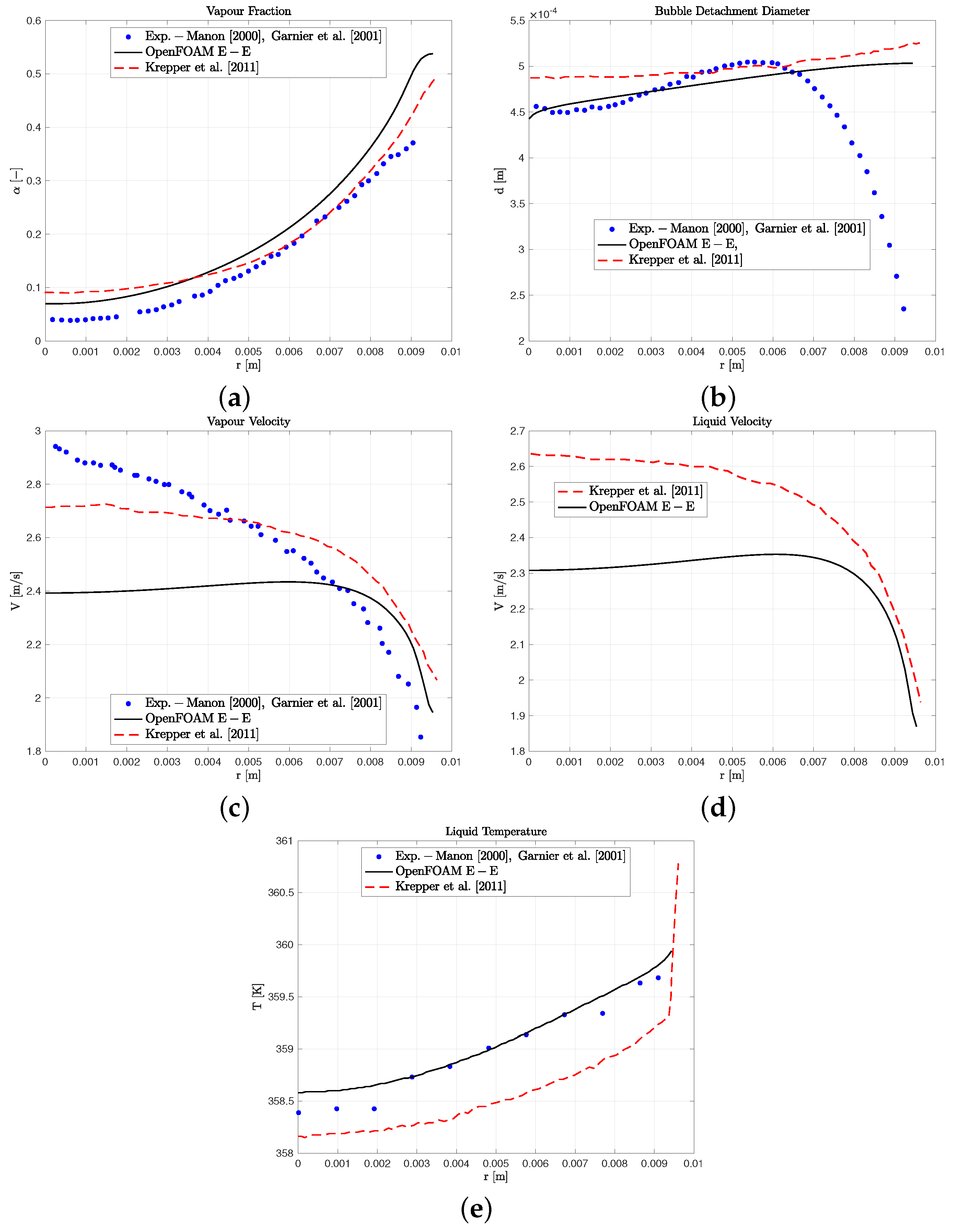
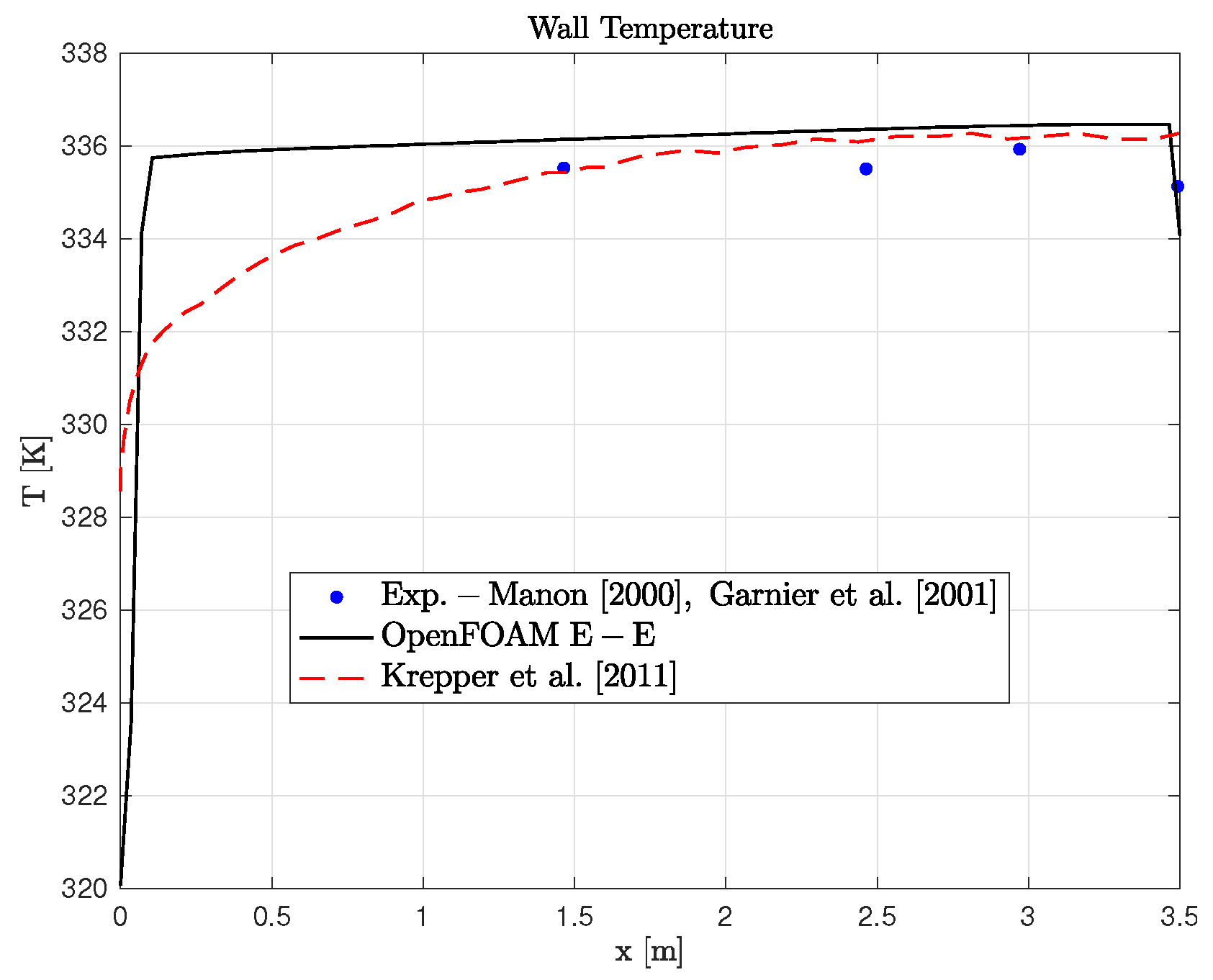
• The numerical model is able to predict the radial profiles of the vapour fraction and liquid temperature, as well as the axial profiles of the heat transfer coefficient and wall super-heat/temperature, after recalibrating the constitutive correlations.
• The model cannot effectively predict the trend of the radial profiles for the velocity and bubble detachment diameter. This is attributed to the fact that the present model does not account for bubble coalescence effects, meaning the buoyancy effects result in higher velocities than predicted towards the centre of the tube. Additionally, the attraction and coalescing of small bubbles from bigger bubbles, causing a significant reduction in the bubble detachment diameter towards the tube’s wall, cannot be captured here.
• The model shows high sensitivity when the operating conditions change (even non-significantly such as the DEBORA 3 vs. 4 cases), and the tuning of the correlations is essential to accurately predict the experimental data.
• From the sensitivity analysis of the parameters comprising the empirical closures of the sub-models, the reference diameter $d_{ref}$ of the bubble detachment diameter closure was shown to have significant influence in all the examined fluid and heat transfer characteristics. Additionally, we saw that all the closures have a significant impact on the wall super-heat/temperature profile measured in the axial distance. Conversely, the closure parameters $C_n$, $N_{ref}$ and $\Delta T_{ref}$ of the nucleation site density sub-model, and the $C_f$ constant of the bubble detachment frequency sub-model, have either an intermediate or minor impact on the radial profiles of the volume fraction, bubble detachment diameter, velocity and liquid temperature profiles.
• By adding a bubble coalescence and break-up model, the velocity profile can be significantly improved after performing a sensitivity analysis; however, other parameters such as the vapour fraction are significantly affected as well.

(b) From investigating flow boiling within a single micro-channel:

• The present model is unable to predict the heat transfer coefficient trend, even when $d_{ref}$ of the bubble detachment diameter sub-model is modified. This is attributed to the different underlying physical phenomena of flow boiling within micro-channels compared to conventional tubes, and by the fact that the included sub-models use empirical correlations based on experiments conducted in conventional tubes.
• The development of suitable closures based on data specifically obtained from micro- channels at various operating conditions is necessary to utilise the RPI model in such micro-scale investigations.

After observing that the existing closures are unsuitable to simulate flow boiling within micro-channels, future studies should focus on developing and replacing existing sub-models/closures with sub-models based on data from experimental/numerical works on micro-channels to successfully capture such phenomena.

References

1. Mudawar, I. Recent advances in high-flux, two-phase thermal management. J. Therm. Sci. Eng. Appl. 2013, 5, 15. [Google Scholar] [CrossRef]
2. Forster, H.K.; Zuber, N. Dynamics of vapor bubbles and boiling heat transfer. AIChE J. 1955, 1, 531–535. [Google Scholar] [CrossRef]
3. Theodore, L.B.; Adrienne, S.; Lavine, F.P.; Incropera, D.P.D. Fundamentals of Heat and Mass Transfer, 6th ed.; Wiley: New York, NY, USA, 2017; p. 954. [Google Scholar]
4. Zhou, K.; Coyle, C.; Li, J.; Buongiorno, J.; Li, W. Flow boiling in vertical narrow microchannels of different surface wettability characteristics. Int. J. Heat Mass Transf. 2017, 109, 103–114. [Google Scholar] [CrossRef] [Green Version]
5. Fang, X.; Yuan, Y.; Xu, A.; Tian, L.; Wu, Q. Review of correlations for subcooled flow boiling heat transfer and assessment of their applicability to water. Fusion Eng. Des. 2017, 122, 52–63. [Google Scholar] [CrossRef]
6. Dedov, A.V. A Review of Modern Methods for Enhancing Nucleate Boiling Heat Transfer. Therm. Eng. 2019, 66, 881–915. [Google Scholar] [CrossRef]
7. Tibiriçá, C.B.; Ribatski, G. Flow boiling in micro-scale channels-Synthesized literature review. Int. J. Refrig. 2013, 36, 301–324. [Google Scholar] [CrossRef]
8. Drew, D.A. Mathematical Modeling of Two-Phase Flow. Annu. Rev. Fluid Mech. 1983, 15, 261–291. [Google Scholar] [CrossRef]
9. Ishii, M. Thermo-Fluid Dynamic Theory of Two-Phase Flow. Available online: https://inis.iaea.org/search/search.aspx?orig_q=RN:7233706 (accessed on 4 October 2019).
10. Alali, A. Development and Validation of a New Solver Based on the Interfacial Area Transport Equation for the Numerical Simulation of Sub-Cooled Boiling With. Technical Univeristy Munich. 2014. Available online: http://mediatum.ub.tum.de/doc/1172612/1172612.pdf (accessed on 4 October 2019).
11. Warrier, G.R.; Dhir, V.K. Heat transfer and wall heat flux partitioning during subcooled flow nucleate boiling—A review. J. Heat Transf. 2006, 128, 1243–1256. [Google Scholar] [CrossRef]
12. Basu, N.; Warrier, G.R.; Dhir, V.K. Wall heat flux partitioning during subcooled flow boiling: Part 1—Model development. J. Heat Transf. 2005, 127, 131–140. [Google Scholar] [CrossRef] [Green Version]
13. Murallidharan, J.S.; Prasad, B.V.S.S.S.; Patnaik, B.S.V.; Hewitt, G.F.; Badalassi, V. CFD investigation and assessment of wall heat flux partitioning model for the prediction of high pressure subcooled flow boiling. Int. J. Heat Mass Transf. 2016, 103, 211–230. [Google Scholar] [CrossRef]
14. Kurul, N.; Podowski, M.Z. Multidimensional effects in forced convection subcooled boiling. In Proceedings of the 9th International Heat Transfer Conference, Jerusalem, Israel, 19–24 August 1990. [Google Scholar]
15. Yeoh, G.H.; Tu, J.Y. Computational Techniques for Multiphase Flows—Basics and Applications; Elsevier Science and Technology, Butterworth-Heinemann: Oxford, UK, 2010. [Google Scholar] [CrossRef]
16. Krepper, E.; Rzehak, R. CFD for subcooled flow boiling: Analysis of DEBORA tests. J. Comput. Multiph. Flows 2014, 6, 329–359. [Google Scholar] [CrossRef] [Green Version]
17. Tu, J.Y.; Yeoh, G.H. On numerical modelling of low-presure subcooled boiling flows. Int. J. Heat Mass Transf. 2002, 45, 1197–1209. [Google Scholar] [CrossRef]
18. Končar, B.; Kljenak, I.; Mavko, B. Modelling of local two-phase flow parameters in upward subcooled flow boiling at low pressure. Int. J. Heat Mass Transf. 2004, 47, 1499–1513. [Google Scholar] [CrossRef]
19. Drzewiecki, T.; Asher, I.; Grunloh, T.; Petrov, V.; Fidkowski, K.; Manera, A.; Downar, T. Parameter sensitivity study of boiling and two-phase flow models in CFD. J. Comput. Multiph. Flows 2012, 4, 411–426. [Google Scholar] [CrossRef] [Green Version]
20. Krepper, E.; Končar, B.; Egorov, Y. CFD modelling of subcooled boiling-Concept, validation and application to fuel assembly design. Nucl. Eng. Des. 2007, 237, 716–731. [Google Scholar] [CrossRef]
21. Bartolomej, G.G.; Chanturiya, V.M. Experimental study of true void fraction when boiling subcooled water in vertical tubes. Therm. Eng. 1967, 14, 123–128. [Google Scholar]
22. Bartolomej, G.G.; Brantov, V.G.; Molochnikov, Y.S. An experimental investigation of true volumetric vapour content with subcooled boiling in tubes. Therm. Eng. 1982, 29, 132–135. [Google Scholar]
23. Krepper, E.; Rzehak, R. CFD for subcooled flow boiling: Simulation of DEBORA experiments. Nucl. Eng. Des. 2011, 241, 3851–3866. [Google Scholar] [CrossRef]
24. Krepper, E.; Rzehak, R.; Lifante, C.; Frank, T. CFD for subcooled flow boiling: Coupling wall boiling and population balance models. Nucl. Eng. Des. 2013, 255, 330–346. [Google Scholar] [CrossRef]
25. Gu, J.; Wang, Q.; Wu, Y.; Lyu, J.; Li, S.; Yao, W. Modeling of subcooled boiling by extending the RPI wall boiling model to ultra-high pressure conditions. Appl. Therm. Eng. 2017, 124, 571–584. [Google Scholar] [CrossRef]
26. Lemmert, M.; Chawla, J.M. Influence of Flow Velocity on Surface Boiling Heat Transfer Coefficient. Heat Transf. Boil. 1977, 237, 247. [Google Scholar]
27. Unal, H.C. Maximum Bubble Diameter, Maximum Rate During the Subcooled Nucleate Flow Boiling. Int. J. Heat Mass Transf. 1976, 19, 643–649. [Google Scholar] [CrossRef]
28. Cole, R. A photographic study of pool boiling in the region of the critical heat flux. AIChE J. 1960, 6, 533–538. [Google Scholar] [CrossRef]
29. Ariyo, D.O.; Bello-Ochende, T. Constructal design of subcooled microchannel heat exchangers. Int. J. Heat Mass Transf. 2020, 146, 118835. [Google Scholar] [CrossRef]
30. Ferreira, T.P.A.; Ribeiro, G.B. Investigation of bubble parameters and interfacial heat transfer correlations based on radial void fraction profiles of R-134a subcooled boiling flows. J. Braz. Soc. Mech. Sci. Eng. 2021, 43, 18. [Google Scholar] [CrossRef]
31. Wang, Z.; Turan, A. Influence of non-uniform wall heat flux on critical heat flux prediction in upward flowing round pipe two-phase flow. Int. J. Heat Mass Transf. 2021, 164, 7. [Google Scholar] [CrossRef]
32. Setoodeh, H.; Ding, W.; Lucas, D.; Hampel, U. Modelling and simulation of flow boiling with an Eulerian-Eulerian approach and integrated models for bubble dynamics and temperature-dependent heat partitioning. Int. J. Therm. Sci. 2020, 161, 106709. [Google Scholar] [CrossRef]
33. Georgoulas, A.; Andredaki, M.; Marengo, M. An enhanced VOF method coupled with heat transfer and phase change to characterise bubble detachment in saturated pool boiling. Energies 2017, 10, 272. [Google Scholar] [CrossRef] [Green Version]
34. Wang, Z.; Duan, G.; Koshizuka, S.; Yamaji, A. Chapter 18—Moving Particle Semi-Implicit Method; Woodhead Publishing Series in Energy; Woodhead Publishing: Cambridge, UK, 2021; pp. 439–461. [Google Scholar] [CrossRef]
35. Manon, E. Contribution à l’Analyse et à la Modélisation Locale des éCoulements Bouillants Sous-saturés dans les Conditions des Réacteurs à Eau sous Pression. Ph.D. Thesis, Ecole Centrale Paris, Paris, France, 2000; p. 286. Available online: http://www.theses.fr/2000ECAP0696 (accessed on 4 October 2022).
36. Garnier, J.; Manon, E.; Cubizolles, G. Local measurements on flow boiling of refrigerant 12 in a vertical tube. Multiph. Sci. Technol. 2001, 13, 111. [Google Scholar] [CrossRef]
37. Sato, Y.; Sadatomi, M.; Sekoguchi, K. Momentum and heat transfer in two-phase bubble flow—I. Theory. Int. J. Multiph. Flow 1981, 7, 167–177. [Google Scholar] [CrossRef]
38. Menter, F.R.; Esch, T. Elements of Industrial Heat Transfer Predictions. In Proceedings of the 16th Brazilian Congress of Mechanical Engineering, Uberlândia, Brazil, 26–30 November 2001. [Google Scholar]
39. Wang, Q.; Yao, W. Computation and validation of the interphase force models for bubbly flow. Int. J. Heat Mass Transf. 2016, 98, 799–813. [Google Scholar] [CrossRef]
40. Yeoh, G.H.; Cheung, C.P.; Tu, J. Multiphase Flow Analysis Using Population Balance Modeling. Bubbles, Drops and Particles, 1st ed.; Elsevier: Oxford, UK, 2014. [Google Scholar] [CrossRef]
41. Drew, D.A.; Lahey, R.T. The virtual mass and lift force on a sphere in rotating and straining inviscid flow. Int. J. Multiph. Flow 1987, 13, 113–121. [Google Scholar] [CrossRef]
42. Tomiyama, A. Struggle with computational bubble dynamics. Multiph. Sci. Technol. 1998, 10, 369–405. [Google Scholar] [CrossRef]
43. Legendre, D.; Magnaudet, J. The lift force on a spherical bubble in a viscous linear shear flow. J. Fluid Mech. 1998, 368, 81–126. [Google Scholar] [CrossRef]
44. Antal, S.P.; Lahey, R.T.; Flaherty, J.E. Analysis of phase distribution in fully developed laminar bubbly two-phase flow. Int. J. Multiph. Flow 1991, 17, 635–652. [Google Scholar] [CrossRef]
45. Lopez de Bertodano, M.; Lahey, R.T.; Jones, O.C. Turbulent bubbly two-phase flow data in a triangular duct. Nucl. Eng. Des. 1994, 146, 43–52. [Google Scholar] [CrossRef]
46. Gilman, L.A. Development of a General Purpose Subgrid Wall Boiling Model from Improved Physical Understanding for Use in Computational Fluid Dynamics. Ph.D. Thesis, Massachusetts Institute of Technology, Cambridge, MA, USA, 2014. Available online: https://dspace.mit.edu/handle/1721.1/92099 (accessed on 4 October 2019).
47. Valle, V.H.D.; Kenning, D.B.R. Subcooled flow boiling at high heat flux. Int. J. Heat Mass Transf. 1985, 28, 1907–1920. [Google Scholar] [CrossRef]
48. Kocamustafaogullari, G.; Ishii, M. Foundation of the interfacial area transport equation and its closure relations. Int. J. Heat Mass Transf. 1995, 38, 481–493. [Google Scholar] [CrossRef]
49. Tolubinsky, V.I.; Kostanchuk, D.M. Vapour bubbles growth rate and heat transfer intensity at subcooled water boiling. In Proceedings of the International Heat Transfer Conference 4, Paris, France, 31 August–5 September 1970; p. 23. [Google Scholar]
50. Wu, Q.; Kim, S.; Ishii, M.; Beus, S.G. One-group interfacial area transport in vertical bubbly flow. Int. J. Heat Mass Transf. 1998, 41, 1103–1112. [Google Scholar] [CrossRef]
51. Ishii, M.; Kim, S.; Kelly, J. Development of Interfacial Area Transport Equation. Nucl. Eng. Technol. 2005, 37, 11. [Google Scholar]
52. Larsen, B.E.; Fuhrman, D.R.; Roenby, J. Performance of interFoam on the simulation of progressive waves. Coast. Eng. J. 2018, 61, 18. [Google Scholar] [CrossRef] [Green Version]
53. Holzmann, T. Mathematics, Numerics, Derivations and OpenFOAM—The basics for numerical simulations. Holzmann CFD 2017, 7, 155. [Google Scholar]
54. Nagayama, G.; Matsumoto, T.; Fukushima, K.; Tsuruta, T. Scale effect of slip boundary condition at solid-liquid interface. Sci. Rep. 2017, 7, 43125. [Google Scholar] [CrossRef] [Green Version]
55. Tuckerman, D.B.; Pease, R.F.W. High-Performance Heat Sinking for VLSI. IEEE Electron Device Lett. 1981, 2, 126–129. [Google Scholar] [CrossRef]
56. Wu, Z.; Sundén, B. On further enhancement of single-phase and flow boiling heat transfer in micro/minichannels. Renew. Sustain. Energy Rev. 2014, 40, 11–27. [Google Scholar] [CrossRef]
57. Kandlikar, S.G. History, advances, and challenges in liquid flow and flow boiling heat transfer in microchannels: A critical review. J. Heat Transf. 2012, 134. [Google Scholar] [CrossRef]
58. Karayiannis, T.G.; Mahmoud, M.M. Flow boiling in microchannels: Fundamentals and applications. Appl. Therm. Eng. 2017, 115, 1372–1397. [Google Scholar] [CrossRef]
59. Sun, L.; Mishima, K. An evaluation of prediction methods for saturated flow boiling heat transfer in mini-channels. Int. J. Heat Mass Transf. 2009, 52, 5323–5329. [Google Scholar] [CrossRef]
60. Ribatski, G.; Wojtan, L.; Thome, J.R. An analysis of experimental data and prediction methods for two-phase frictional pressure drop and flow boiling heat transfer in micro-scale channels. Exp. Therm. Fluid Sci. 2006, 31, 1–19. [Google Scholar] [CrossRef]
61. Vontas, K.; Andredaki, M.; Georgoulas, A.; Miché, N.; Marengo, M. The effect of surface wettability on flow boiling characteristics within microchannels. Int. J. Heat Mass Transf. 2021, 172, 18. [Google Scholar] [CrossRef]
62. Vontas, K.; Latella, F.; Georgoulas, A.; Miché, N.; Marengo, M. A numerical study on flow boiling within micro-passages: The effect of solid surface thermophysical properties. In Proceedings of the 15th International Conference on Heat Transfer, Fluid Mechanics and Thermodynamics, Amsterdam, The Netherlands, 25–28 July 2021; p. 6. [Google Scholar]
63. Vontas, K.; Andredaki, M.; Georgoulas, A.; Miché, N.; Marengo, M. The Effect of Hydraulic Diameter on Flow Boiling within Single Rectangular Microchannels and Comparison of Heat Sink Configuration of a Single and Multiple Microchannels. Energies 2021, 14, 6641. [Google Scholar] [CrossRef]
64. Mahmoud, M.M.; Karayiannis, T.G.; Kenning, D.B.R. Surface effects in flow boiling of R134a in microtubes. Int. J. Heat Mass Transf. 2011, 54, 3334–3346. [Google Scholar] [CrossRef] [Green Version]
Figure 1. (a) Experimental setup by Manon [35] and Garnier et al. [36]. (b) Computational domain of the 2D axisymmetric simulations conducted in the present study.
Energies 16 04996 g001
Figure 2. Contours of (a) velocity at 0.5 s, (b) vapour volume fraction at 4 s, (c) temperature of the liquid at 4 s and (d) vapour velocity at 4 s for the DEBORA 2 case.
Energies 16 04996 g002
Figure 3. Mesh independency study comparison for (a) Vapour Fraction, (b) Liquid Temperature and (c) Vapour Velocity.
Energies 16 04996 g003
Figure 4. DEBORA 1-radial line: Numerical results and comparison between the present simulation, experiments of Manon [35] and Garnier et al. [36] and Krepper and Rzehak [23]. (a) Vapour Fraction, (b) Bubble Departed Diameter, (c) Vapour Velocity, (d) Liquid velocity, (e) Liquid Temperature.
Energies 16 04996 g004
Figure 5. DEBORA 1-axial line: Numerical results and comparison between the present simulation, experiments of Manon [35] and Garnier et al. [36] and Krepper and Rzehak [23]. (a) Heat Transfer Coefficient, (b) Wall Superheat.
Energies 16 04996 g005
Figure 6. DEBORA 2-radial line: Numerical results and comparison between the present simulation, experiments of Manon [35] and Garnier et al. [36] and Krepper and Rzehak [23]. (a) Vapour Fraction, (b) Bubble Departed Diameter, (c) Vapour Velocity, (d) Liquid velocity, (e) Liquid Temperature.
Energies 16 04996 g006
Figure 7. DEBORA 2-axial line: Numerical results and comparison between the present simulation, experiments of Manon [35] and Granier et al. [36] and Krepper and Rzehak [23]. (a) Heat Transfer Coefficient, (b) Wall Superheat.
Energies 16 04996 g007
Figure 8. DEBORA 3-radial line: Numerical results and comparison between the present simulation, experiments of Manon [35] and Garnier et al. [36] and Krepper and Rzehak [23]. (a) Vapour Fraction, (b) Bubble Departed Diameter, (c) Vapour Velocity, (d) Liquid Temperature.
Energies 16 04996 g008
Figure 9. DEBORA 3-axial line: Numerical results and comparison between the present simulation, experiments of Manon [35] and Granier et al. [36] and Krepper and Rzehak [23].
Energies 16 04996 g009
Figure 10. DEBORA 4-radial line: Numerical results and comparison between the present simulation, experiments of Manon [35] and Garnier et al. [36] and Krepper and Rzehak [23]. (a) Vapour Fraction, (b) Bubble Departed Diameter, (c) Vapour Velocity, (d) Liquid Temperature.
Energies 16 04996 g010
Figure 11. DEBORA 4-axial line: Numerical results and comparison between the present simulation, experiments of Manon [35] and Granier et al. [36] and Krepper and Rzehak [23].
Energies 16 04996 g011
Figure 12. Radial line: Comparison between the numerical results of the IATE model, the optimal E-E case (without the IATE model), experiments of Manon [35] and Garnier et al. [36] and Krepper and Rzehak [23]. (a) Vapour Fraction, (b) Liquid Temperature, (c) Vapour Velocity.
Energies 16 04996 g012
Figure 13. Experimental and numerical setup. (a) Experimental domain as provided by Mahmoud et al. [64] (b) computational domain and dimensions, (c) mesh details and boundary conditions.
Energies 16 04996 g013
Figure 14. Comparison between the numerical simulation results for two different d r e f values for (a) G = 200 kg m−2 s−1 and (b) G = 300 kg m−2 s−1 and the experiment performed by [64].
Energies 16 04996 g014