1. Introduction
In order to prevent and control transmission line icing disasters, various countries have vigorously developed transmission line icing monitoring technology. Currently, the most widely applicable and accurate monitoring method is still the online monitoring device for icing tension. The influence of wind in nature on the measurement of ice load on transmission lines cannot be ignored, and the tension sensor of transmission lines often measures the coupled load of wire ice and wind. Therefore, conducting research on the impact of instantaneous wind on the dynamic tension of transmission line icing conductors, eliminating the impact of instantaneous wind on the measurement of conductor icing quality, can improve the accuracy of all-weather transmission line icing quality measurement, and provide a reference for the power sector to take reasonable de-icing measures in a timely manner. It has certain engineering application value for building a safe and reliable power grid.
At present, scholars have conducted research on the dynamic tension response of transmission lines using on-site experiments, numerical analysis calculations, and wind tunnel tests [
1,
2,
3,
4,
5,
6,
7]. Wang Dahai et al. [
8] decomposed the transmission line under wind action into static and dynamic actions and obtained a spring pendulum model for calculating the dynamic tension of transmission lines in the time domain. Compared with the corresponding finite element model calculation results, the spring pendulum model has sufficient calculation accuracy. Hung et al. [
9] analyzed the relationship between the frequency domain response of wind-induced tension of transmission lines and wind speed through measured wind field data and corresponding wire tension data. Zhao Guifeng et al. [
10] constructed an aeroelastic model based on the actual transmission line of a certain project and conducted wind tunnel tests with a wind field that was suitable for the actual situation. The research showed that the dynamic tension of the transmission line has strong nonlinear characteristics under pulsating wind fields, and the vibration of the transmission tower is largely due to the dynamic tension of the line. Wang Shuliang et al. [
11] measured the in-plane and out-of-plane displacement of wires in wind tunnels based on DICM (Digital Image Correlation Method). The in-plane and out-of-plane displacement can be used to calculate wire tension. The results showed that at low wind speeds, the wire mainly vibrates out of the plane, while at high wind speeds, coupled vibrations occur both out of the plane and in the plane. The nonlinearity of wire tension increases with the increase in wind speed. Overall, the dynamic tension of transmission lines has strong nonlinear characteristics under fluctuating wind fields, which is significantly different from the tension calculated using static wind. It can be seen that the current research on the wind-induced vibration response of transmission lines under wind load is mostly focused on the tower line system, and there is a lack of research on dynamic tension response. Moreover, most of the consideration is the non-icing state of transmission lines, and there are still shortcomings in the research on the dynamic tension of iced conductors.
Therefore, this article conducts natural icing tests at field stations and uses dynamic tension formulas to calculate the aerodynamic resistance coefficient of conductors under different icing conditions. It studies the effects of instantaneous wind speed and icing thickness on the dynamic tension and aerodynamic resistance coefficient of conductors, constructs a finite element model based on the experimental conductor parameters and verifies it. It supplements the analysis of the dynamic tension characteristics of icing conductors under the instantaneous wind. The research results of this article have important guiding value for the construction of anti-icing warning systems for transmission lines.
2. Mechanical Calculation of Iced Conductors
In order to perform the mechanical calculation and analysis of iced conductors, the following assumptions are made [
12]:
① The wire is an ideal flexible cable structure which cannot be compressed or bent(In a normal isolated range, due to the high axial tension of the conductor, the bending stiffness of the tension string can be ignored). The ratio of the cross-sectional size of the wire to its length is minimized, so the bending stiffness of the cross-section can be ignored in the calculation.
② The material of the wire complies with Hooke’s Law(Within the elastic limit, the stress and strain of an elastic object are proportional to each other), and the wire’s working range is in the elastic stage.
③ The ice layer is evenly distributed along the whole span of the OHL and does not modify the properties of the material and structure.
2.1. Static Mechanical Calculation of Iced Conductors
The research shows that when the conductor sag is less than 0.125, the difference between the parabola and the catenary is very small, and the parabola formula of the conductor meets the accuracy requirements [
13]. When the conductor is covered with ice uniformly, it can be assumed that the conductor only has vertical loads, and the configuration of the covered conductor can be expressed using the parabolic formula [
14]. In practical applications, measuring the horizontal tension of transmission wires is difficult, and usually, only the axial tension at the termination of the transmission wire can be detected. The tensional force at the lowest-hanging point of the wire is calculated as:
where
L is the span of the transmission wire, m;
H is the height difference of the transmission line, m;
HB is the axial tension at the end of the low hanging point of the wire, N;
H0 is the horizontal tension of the wire, N. f is the conductor sag, m. The values of
f,
L and
H are shown in
Table 1.
When the height difference h = 0, the axial tension HB value is at its maximum. When the vertical-to-span ratio is less than 0.075, the maximum axial tension differs only 4% from the horizontal tensional force. When the height difference h ≠ 0, the axial tension at the lowest-hanging point is closer to the horizontal tensional force. Therefore, when the vertical-to-span ratio is less than 0.075, the lowest-hanging point tensional force of the wire can be used to replace the horizontal one.
Wire icing is often associated with a reduced temperature, and the change in wire length caused by cold shrinkage cannot be ignored. From the perspective of motion, when there is no instantaneous wind, the wire is only affected by its own weight and icing load, resulting in in-plane deformation. From a physical perspective, the elongation of the wire is related to the variation of tensional force, and combined with the influence of temperature, the final deformation coordination equation of the wire is obtained as:
In the formula:
E is the Young’s modulus, Pa; Δ
H is the change in horizontal ten-sion of the conductor before and after icing, N;
A is the calculated cross-sectional area of the wire, m2;
α Is the temperature expansion coefficient of the wire; Δ T is the amount of temperature change before and after icing, °C. After adding a uniform icing load
q to the conductor, the final state of the conductor satisfies the deformation coordination equation. According to Equation (1), the difference formula between the horizontal tension
H1 after icing and the horizontal tension
H0 before icing can be obtained as follows:
where
E is Young’s modulus, Pa; Δ
H is the change in horizontal tension of the conductor before and after icing, N;
A is the calculated cross-sectional area of the wire, m
2; α Is the temperature expansion coefficient of the wire; Δ
t is the amount of temperature change before and after icing, °C.
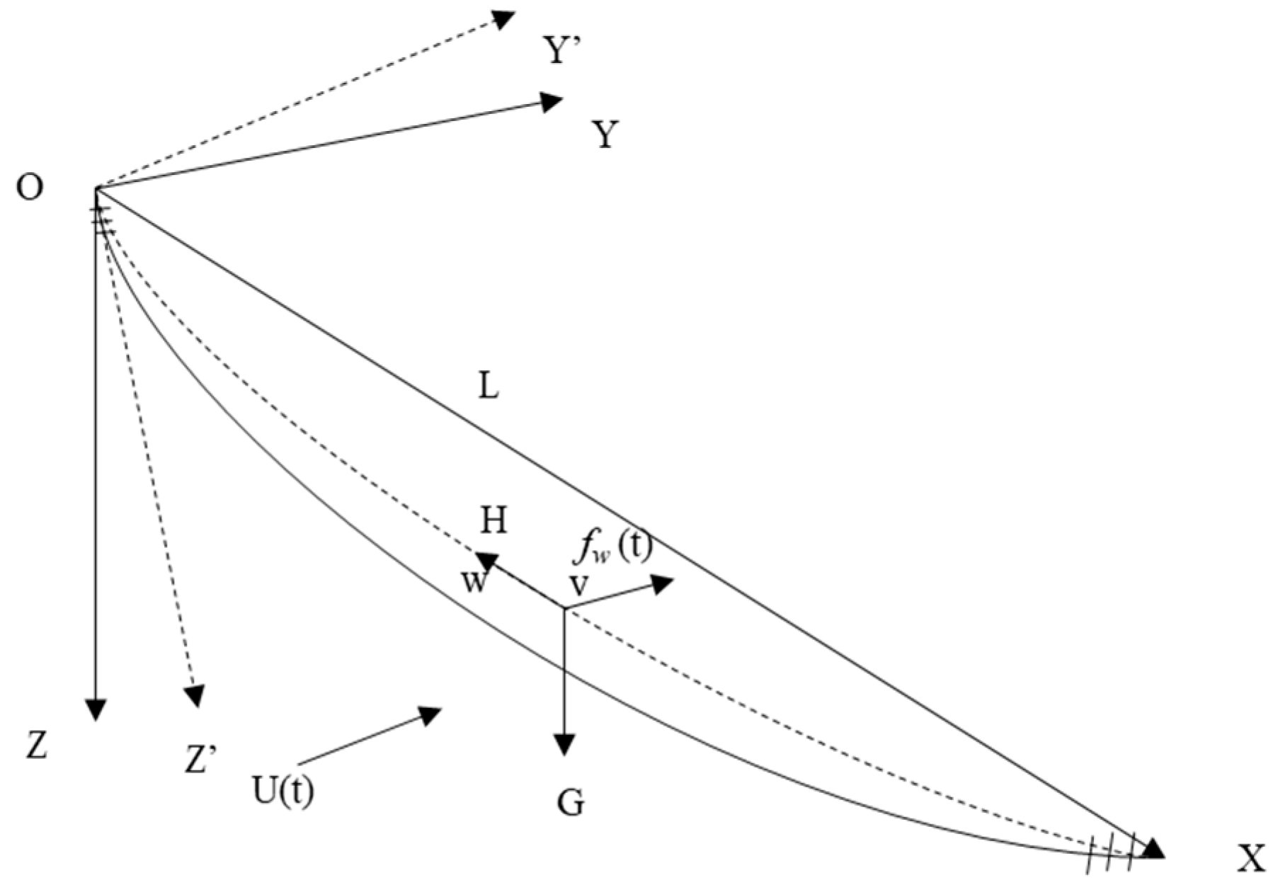
2.2. Calculation of Dynamic Tension of Iced Conductors under Instantaneous Wind Load
Taking the first level of an iced conductor as shown in
Figure 1 as the research object. The YOZ plane configuration projection of the iced conductor, as shown in
Figure 2, is taken as the object for study.
The initial configuration of the conductor adopts a parabolic formula. The initial horizontal tension of the conductor is
H0, and the static horizontal stress of the conductor after icing is
H1. Under the impact of wind load
fw (t), the dynamic horizontal stress of the iced conductor is
H (t), and the displacement of the iced conductor unit along the wind direction (
y-axis) is
v (x, t), and the vertical (
z-axis) displacement is
w (x, t). Ignoring the resonance component of the dynamic tension response of the conductor [
14], the motion equation system of the iced conductor under the combined action of wind, ice, and the self-weight is [
15]:
When
x = 0 and
x =
L, the vertical displacement and windward displacement of the iced wire unit are both 0,
w (0, t) =
w (
L,
t) =
v (0,
t) =
v (
L,
t) = 0. The configuration equation of the iced wire unit is Equation (5)
The vertical displacement of the iced wire unit at any position is obtained by integrating it twice
Calculate the windward displacement of the iced wire element at any position by integrating the second equation of equation system (4) twice as:
Derive the three-dimensional deformation coordination equation of the iced conductor by analogy from Equation (2):
By simplifying Equations (5) and (6) into Equation (7), the quantitative relationship equations for horizontal dynamic tensional force, temperature, ice load, and instantaneous wind load of the iced conductor are obtained as follows:
In the formula: m0 is the mass per unit length of the wire, in kg; mb is the unit icing mass of the conductor, in kg; g is the gravitational acceleration, in m/s2.
3. Experimental Study on Dynamic Tension of Iced Conductors under Instantaneous Wind
This article conducted experiments to measure the dynamic tension and simultaneously the instantaneous wind speed of the single test conductor section and steel strand section (from now on referred to as the test conductor) under natural icing conditions at the Hunan Xuefengshan Energy Equipment Safety National Field Scientific Observation and Research Station of Chongqing University. The specific data for the two test wires is shown in
Table 2.
The DYLY-101 cylindrical S-type tensile sensor is used to measure the axial tensional force at the termination of the test wire, as shown in
Figure 3. Considering the relatively long response time of the tensile sensor, the average tension value of 15 s before and after the corresponding moment of instantaneous wind speed is taken as the tension at that time. The anti-icing wind pressure anemometer is adopted, which can accurately measure the speed of high wind and its direction for 3 s and can continue to work in the low temperature environment. Both devices transmit data wirelessly to the computer through the E22 module, achieving synchronous collection of dynamic tensional force and instantaneous wind speed. To ensure the integrity of wire icing, the unit icing mass needs to be calculated based on the equivalent ice thickness. The equal ice thickness will be converted into Equation (9) based on the length and thickness of the icing. After the test is completed, the ice density will be measured using the discharge method [
16], and the unit length icing mass will be calculated using Equation (10) based on the equivalent ice thickness [
17].
In the formula: bm is the equivalent thickness of the ice cover, in mm; d1 and d2 refer to the thickness of the iced conductor, in mm; ρb is the density of the ice, in kg/m3.
The effective wind speed is calculated using Equation (11) with a north direction as the reference angle (0°).
In the formula: v (t) is the effective wind speed in the horizontal direction, m/s; U (t) is the instantaneous wind speed, m/s.
The average values of the icing parameters of the test wires during the three icing stages are shown in
Table 3. Due to the highly uneven icing of the three steel strands during the ice period, no further investigation will be conducted.
3.1. The Influence of Instantaneous Wind Speed on the Dynamic Tension of Conductors
The study on the influence of instantaneous wind icing on the tension of the conductor needs to eliminate the effect of icing growth. According to the natural icing test at the Xuefengshan National Field Station, it was found that in windy weather, ice accumulation is more pronounced, and a small amount of ice accumulation can cause a significant increase in the tensional force of the test conductor. Based on the site measurement results and statistical analysis of the tensile data, it is found that the conductor icing does not increase within 5 min. Therefore, taking 5 min as the time interval to study the instantaneous wind and the dynamic tensional force is feasible. Due to the influence of accumulated ice, the static stress at the termination of the test wire during different stages of the same ice period is not the same. Therefore, to better understand the relationship between the dynamic tensional force of the ice-covered wire and the instantaneous wind speed, the tensional force of the ice-covered wire in each stage in relation to the static stress when the wind is absent has been studied.
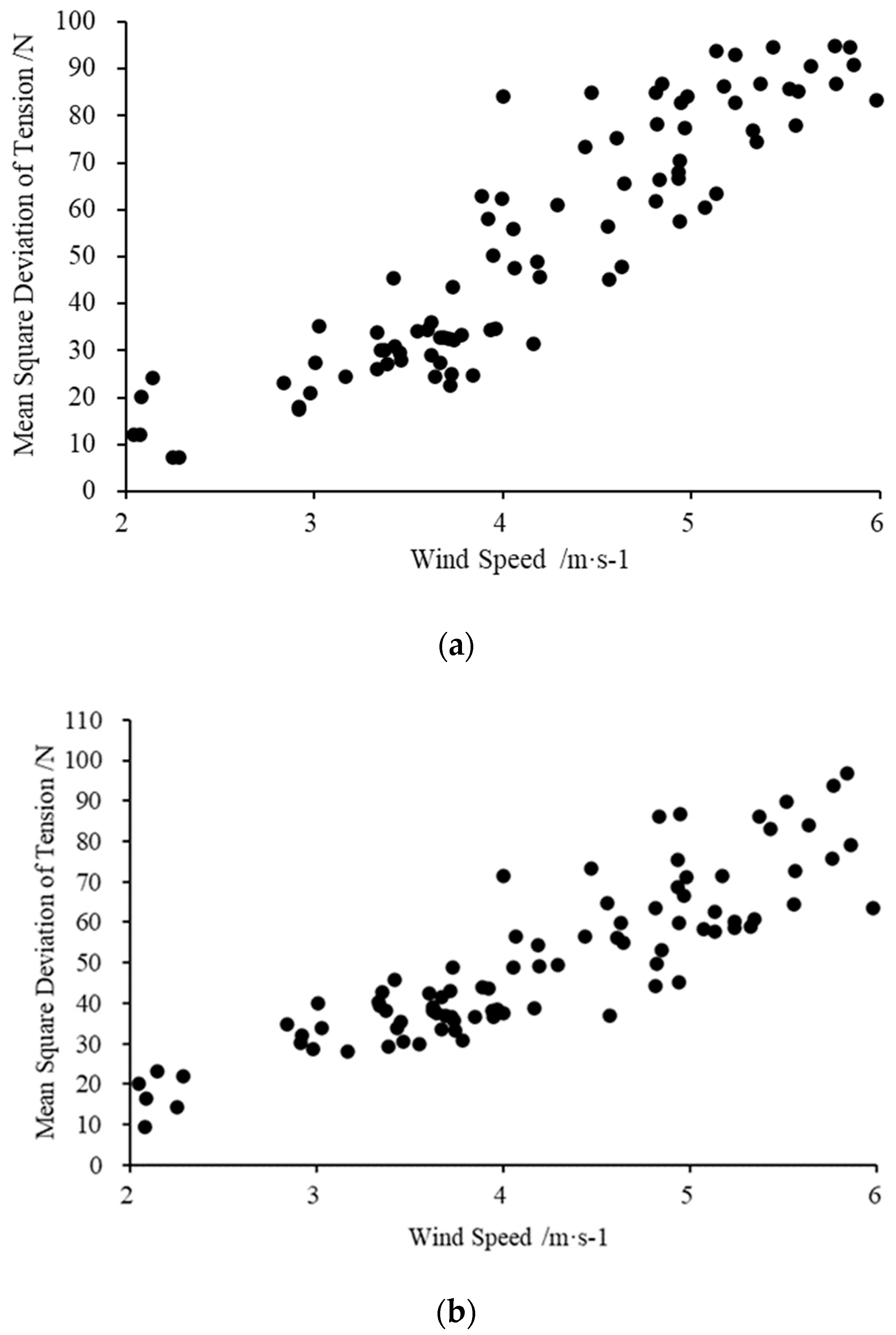
The scatter points of the axial tension increment at the end of the experimental iced wire and the corresponding instantaneous wind speed at the corresponding time are shown in
Figure 4. To more intuitively explore the influence of wind speed on the axial tension at the end of the iced wire, the dynamic statistical values of tension were ana-lyzed, and the scatter points corresponding to the mean square deviation of the tension at the end of the experimental iced wire and the mean wind speed within 5 min were obtained, as shown in
Figure 5. As the instantaneous wind speed increases, the increment of tension at the end of the iced conductor increases, the mean square deviation of axial tension at the end of the test steel strand and single conductor increases, and the dispersion increases.
3.2. The Influence of Instantaneous Ice Coating Thickness on the Dynamic Tensional Force of Conductors
Due to the fact that the ice load and axial tensional force are increasing with the increased ice coating thickness, to better compare the dynamic tensional force with different ice thicknesses, the increment of axial stress at the terminal of the iced conductor is selected as the key parameter for analysis. Experimental measurements have found that the thickness of ice cover during the same ice season in general increases over time, but the cross-wind length of the covered wire does not vary significantly. Therefore, it is assumed that the cross-wind length of the coated wire during the same ice period will remain constant.
The tensional force data from a single conductor, which is captured during the same ice season but at different stages within a 5-min window, is plotted against the wind speed in a scatter diagram (
Figure 6) to analyze the relationship between the dynamic tensional force increment of the tested conductor and the instantaneous wind speed. As the ice thickness increases, the axial tensional force increment rate at the terminal of the conductor decreases. Assuming the ice shape and the cross-wind length remain constant under the same instantaneous wind speed, when the ice thickness increases, it is found that the tension increment reduces.
3.3. The Influence of Instantaneous Wind Speed and Ice Thickness to the Aerodynamic Resistance Coefficient for Iced Conductors
The shape of accumulated ice on the OHL conductor significantly alters its characteristic aerodynamic coefficient. In field experiments, the shape of the ice coating is extremely irregular, and the wind load cannot be calculated precisely through its aerodynamic characteristics. Therefore, it is necessary to first determine the relationship between wind load and effective instantaneous wind speed under different icing conditions. During the period of static ice load, the total wind load is calculated from Equation (8) by using the known tensional force at the lowest mid-point of the sag. According to Equation (13), the wind load of the conductor is related to the square of the wind speed. The calculation formula for the aerodynamic resistance coefficient of the iced conductor is [
18]:
where ρ Is the density of air, in kg/m
3;
v (t) is the instantaneous wind speed at the horizontal direction, calculated by Equation (11), in m/s;
D is the cross- wind length of the iced conductor cross-section, in m;
L is the length of the span, in m;
qw (
t) is the total wind load of the co-relating conductor, in N.
Since the length of the cross-wind section on an iced conductor during the same ice season does not vary significantly compared with its thickness, the aerodynamic drag coefficient is predominantly determined by the thickness of the ice coating. The correlation between the aerodynamic resistance coefficient of steel strands and instantaneous wind speed is shown in
Figure 7, where single conductors are tested during their various icing stages. The aerodynamic resistance coefficient of the iced test wire decreases with increased wind speed, and it eventually approaches a constant. Under the same instantaneous wind speed conditions, the aerodynamic resistance coefficient of the test wire reduces with increased ice thickness.
4. Simulation on Dynamic Tensional Force of Iced Conductors Subject to Instantaneous Wind
4.1. Model Establishment and Validation
Considering the constantly changing thickness of natural icing in field stations, the irregular icing shape, and the small range of variation in instantaneous wind speed, a tailored simulation study is performed to strengthen the understanding of the measurement results. This article uses the finite element software ABAQUS to establish a simplified model with a single conductor. The parameter specifications are listed in
Table 2. The time-domain method is used to analyze the dynamic tensional force of the iced conductor subject to instantaneous wind [
19]. According to
Figure 7, the aerodynamic resistance coefficient of the test wire is used to calculate the wind load, and the mass of ice from the measurement is used for the calculation. The comparison between the simulation and experiment results are shown in
Figure 8. The two curves followed a similar trend, and the maximum relative error is approximately 8.46%. This indicates that the simulation model achieved reasonable accuracy.
The test conductor is installed in a Class B area type [
20], with a wide range of average wind speed. The Kaimal spectrum is used for pulsating wind simulation [
21], and the corresponding total wind speed time history can be obtained by overlaying the pulsating wind speed with the average wind speed. The wind speed right at the end of each second is taken as the instantaneous wind speed value for that 1-s interval.
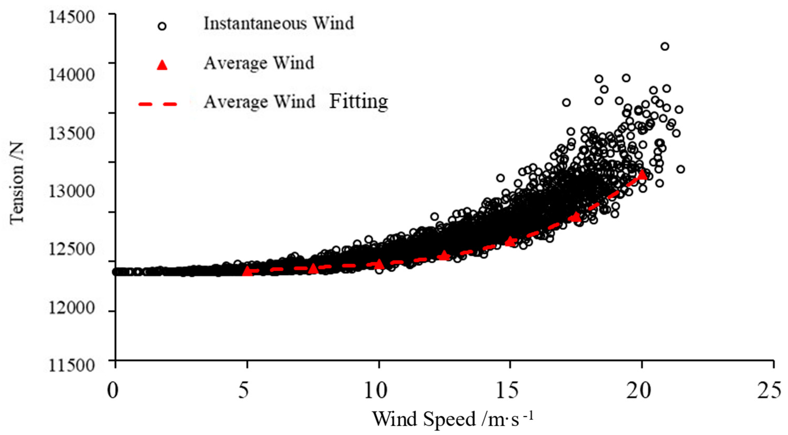
4.2. The Influence of Wind Speed on the Dynamic Tensional Force for Iced Conductors
Taking the iced conductor with the crescent shape as an example, the instantaneous axial tensional force at the terminal of the iced conductor is correlated to the instantaneous wind speed as defined previously. The scatter plot of the axial tensional force at the terminal of the iced conductor under strong wind speed is obtained through experiments. The axial static tensional force of the conductor is calculated by comparing the 10-min averaged wind speed, as shown in
Figure 9. The axial tensional force at the terminal of the crescent-shape iced conductor followed a quadratic growth trend in regards to the instantaneous wind speed, where the degree of dispersion increases gradually. The difference between the maximum static tensional force and the dynamic tensional force of the conductor increases, and the ratio of the difference to its static value rises from 0.82% to 11.19%.
4.3. The Influence of Ice Thickness on the Dynamic Tensional Force of Conductors
A crescent-shaped ice cover with ice thickness b of 5 mm, 10 mm, 15 mm, and 20 mm is built up in the simulation along with the other four working conditions. The increments of axial tensional force are detected within a 60 s window, and they are then aligned with the instantaneous wind speed at each instantaneous moment. The relationship among the increment of axial tensional force on the OHL conductor, different ice cover thicknesses, and the instantaneous wind speed is shown in
Figure 10. It can be seen that for crescent-shaped ice accumulation under the same wind speed conditions, the thicker the ice cover, the smaller the tensional force increment will be. With the increase in ice thickness, the degree of dispersion reduces gradually and approaching a constant value.
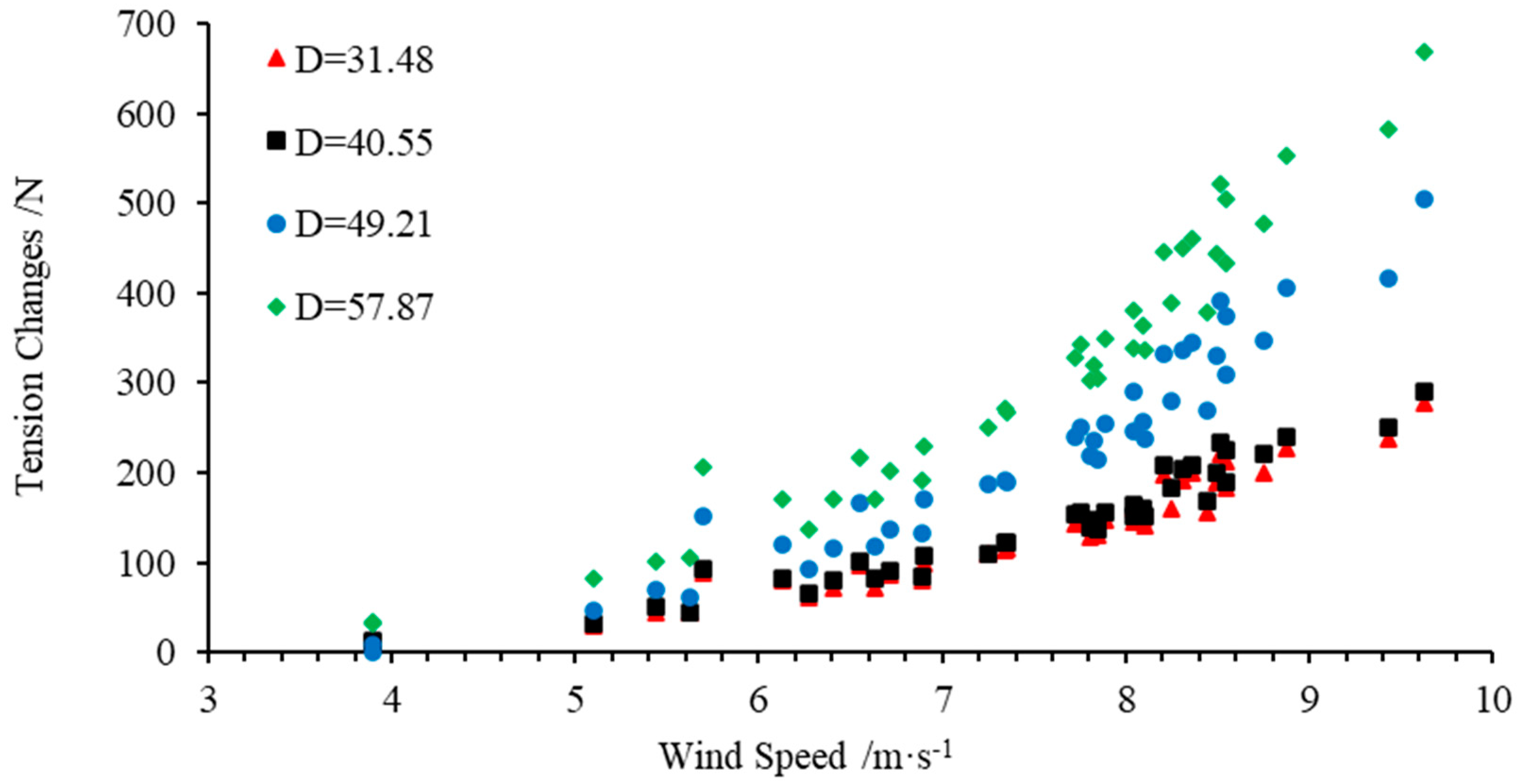
4.4. The Influence of Cross Section Windward Length on the Dynamic Tension of Conductors
The cross-wind length D of the fan-shaped icing section varies with the thickness of the icing. Taking the fan-shaped ice accumulation as an example, the influence of the section’s cross-wind length on the conductor’s dynamic tensional force is studied. The thickness of the ice cover (b) is set to 5 mm, 10 mm, 15 mm, and 20 mm, correlating to four working conditions that have a cross-wind length of 31.48 mm, 40.55 mm, 49.21 mm, and 57.13 mm, respectively. The relationship between the difference in axial tensional force at the terminal of the conductor, the instantaneous wind speed, and the different cross-wind sizes of the cells in shown in
Figure 11.
From
Figure 11, it is found that for fan-shaped icing, under the same wind speed conditions, the larger the cross-wind length of the cross-section, the larger the overall tensional force increment. The axial tensional force increment at the terminal of the conductor increases with the wind speed. As the cross-wind length of the cross-section increases, the degree of dispersion of the axial tensional force increases with the instantaneous wind speed.
5. Discussion
The dynamic tension of the conductor is affected by the combined action of wind load, ice load, and self-weight load. The wind load is positively correlated with the increase in instantaneous wind speed and the length of the section facing the wind, while it is negatively correlated with the thickness of the ice cover. The ice load is mainly affected by the thickness of the ice cover and increases with the increase in the ice cover thickness. Wind speed, ice thickness, and cross-sectional windward length affect the dynamic tension of the conductor by affecting wind and ice loads.
The wind speed affects the magnitude and dispersion of the dynamic tension of the iced conductor. As the instantaneous wind speed increases, the dispersion of the axial dynamic tension at the end of the conductor increases, and the difference between the static tension and the maximum dynamic tension of the conductor increases. When the average wind speed increases from 5 m/s to 20 m/s, the difference between the maximum dynamic tension calculated by using the instantaneous wind speed and the static tension increases from 215.12 N to 772.32 N, and the ratio of the difference to the static tension increases from 1.80% to 5.60%. As the average wind speed increases, the mean square deviation of the tension of the iced conductor shows an increasing trend, and the increasing speed accelerates. The motion state of the iced conductor becomes increasingly unstable, and the amplitude increases. When the wind speed increases from 5 m/s to 20 m/s, the mean square deviation of dynamic tension increases from 51.99 N to 568.27 N. For every 2.5 m/s increase in wind speed, the mean square deviation of dynamic tension increases by 43.64 N, 73.65 N, 82.68 N, 85.54 N, 105.65 N, and 125.12 N, respectively, with an increase in amplitude.
The thickness of icing affects the magnitude and dispersion of the dynamic tension of the iced conductor: as the thickness of icing increases, the extreme and average values of the tension increment of the iced conductor show a downward trend and tend to flatten out. When the ice thickness increases from 5 mm to 20 mm, the average value of tension increment decreases from 18.95 N to 1.68 N, and the extreme value of tension increment decreases from 65.69 N to 9.37 N. For every 5 mm increase in ice thickness, the average value of tension decreases by 12.85 N, 3.14 N, and 1 N, respectively. The extreme value of tension increment decreases by 34.22 N, 15.54 N, and 6.57 N, and the decreased amplitude slows down. As the thickness of the icing increases, the mean square deviation of the dynamic tension of the crescent-shaped icing conductor shows a decreasing trend and tends to be gentle. The movement state of the icing conductor becomes more stable, and the amplitude decreases. When the ice thickness increases from 5 mm to 20 mm, the mean square error of dynamic tension increment decreases from 14.87 N to 2.49 N. For every 5 mm increase in ice thickness, the mean square error of dynamic tension increment decreases by 34.22 N, 15.54 N, and 6.57 N, respectively, with a slower decrease in amplitude.
The windward length of the cross-section affects the magnitude and dispersion of the dynamic tension of the iced conductor. As the windward length of the cross-section increases, the extreme and average values of the tension increment of the iced conductor show an increasing trend, and the growth rate accelerates. When the windward length of the section increases from 31.48 mm to 57.87 mm, the average value of tension increment increases from 18.95 N to 280.49 N, and the extreme value of tension increment increases from 553.96 N to 1361.33 N. For each increase of 8.55 mm in the windward length of the section, the average value of tension increases by 8.68 N, 54.17 N, and 112.64 N, respectively, and the extreme value of tension increases by 16.30 N, 183.86 N, and 607.20 N, respectively, with an increase in amplitude. As the windward length of the cross-section increases, the mean square deviation of the tension of the iced conductor also shows an increasing trend, and the growth rate accelerates. The motion state of the iced conductor becomes increasingly unstable, and the amplitude increases. When the ice thickness increases from 31.48 mm to 57.87 mm, the mean square deviation of dynamic tension increment increases from 92.33 N to 226.12 N. For each increase in ice thickness of 8.55 mm, the mean square deviation of dynamic tension increment increases by 3.30 N, 52.40 N, and 78.09 N, respectively, with an increase in amplitude.
6. Conclusions
This article studies the influence of instantaneous wind speed and icing conditions on the dynamic tensional force for OHL conductors, subject to natural icing conditions. The aerodynamic resistance coefficient is calculated using the formula for the dynamic stress of conductors. The influence of instantaneous wind speed and icing thickness on OHL conductors’ dynamic strain and aerodynamic resistance coefficient is investigated. A finite element analysis (FEA) model is built to validate this, various operational conditions are established within the model, and the simulation results are a good supplement for understanding the nature of the dynamic tensional force subject to instantaneous wind speed. The main conclusions are the following:
(1) Under natural icing conditions, the dynamic tensional force of OHL conductors increases with the instantaneous wind speed, and the same trend exists for the vibration magnitudes. When the ice is crescent or wing-shaped, as the ice thickness increases, the axial dynamic tensional force at the conductor terminal reduces when the instantaneous wind speed increases.
(2) The aerodynamic resistance coefficient of the wire subjected to the icing test reduces when the wind speed increases, and it is gradually approaching a constant value eventually. Under the same instantaneous wind speed condition, the aerodynamic resistance coefficient of the test wire decreases with increased ice thickness.
(3) The influence of instantaneous wind speed and icing thickness on the OHL conductors’ dynamic tensional force is verified within the FEA simulation; the same trend is identified for both simulation and experiment. When OHL conductors are subjected to strong wind and ice, the dynamic stress and magnitude of vibration increase with the wind speed. The higher the wind speed, the greater the error when using the average wind speed to calculate the static tensional force. Under the conditions of the case study within this article (10 mm crescent-shaped icing), when the average wind speed is 20 m/s, the ratio of the mismatch to the static tension is 11.19%. For the crescent-shaped icing, as the thickness of the ice increases, the dynamic tensional force reduces when wind speed increases. For the fan-shaped icing, with the increase in the effective cross section, the degree of dispersion and growth rate for the increment of dynamic tensional force are increasing.


