A GPU-Accelerated Particle Advection Methodology for 3D Lagrangian Coherent Structures in High-Speed Turbulent Boundary Layers

Abstract

In this work, we introduce a scalable and efficient GPU-accelerated methodology for volumetric particle advection and finite-time Lyapunov exponent (FTLE) calculation, focusing on the analysis of Lagrangian coherent structures (LCS) in large-scale direct numerical simulation (DNS) datasets across incompressible, supersonic, and hypersonic flow regimes. LCS play a significant role in turbulent boundary layer analysis, and our proposed methodology offers valuable insights into their behavior in various flow conditions. Our novel owning-cell locator method enables efficient constant-time cell search, and the algorithm draws inspiration from classical search algorithms and modern multi-level approaches in numerical linear algebra. The proposed method is implemented for both multi-core CPUs and Nvidia GPUs, demonstrating strong scaling up to 32,768 CPU cores and up to 62 Nvidia V100 GPUs. By decoupling particle advection from other problems, we achieve modularity and extensibility, resulting in consistent parallel efficiency across different architectures. Our methodology was applied to calculate and visualize the FTLE on four turbulent boundary layers at different Reynolds and Mach numbers, revealing that coherent structures grow more isotropic proportional to the Mach number, and their inclination angle varies along the streamwise direction. We also observed increased anisotropy and FTLE organization at lower Reynolds numbers, with structures retaining coherency along both spanwise and streamwise directions. Additionally, we demonstrated the impact of lower temporal frequency sampling by upscaling with an efficient linear upsampler, preserving general trends with only 10% of the required storage. In summary, we present a particle search scheme for particle advection workloads in the context of visualizing LCS via FTLE that exhibits strong scaling performance and efficiency at scale. Our proposed algorithm is applicable across various domains, requiring efficient search algorithms in large, structured domains. While this article focuses on the methodology and its application to LCS, an in-depth study of the physics and compressibility effects in LCS candidates will be explored in a future publication.

1. Introduction

The study of coherency in seemingly random velocity fields of fluid flow has long been applied and of theoretical interest to a broad community. This statement is essentially what the study of turbulence seeks to unravel. High-speed turbulence, relevant in both civilian and military domains, presents a set of unique challenges for both experimental and computational approaches. That being said, the advent of ever-more-powerful computers has made high-fidelity numerical simulations on non-trivial domains feasible. However, once high-quality data are available, efficient tooling must be leveraged to gather knowledge from the vast volumes of data usually generated by numerical simulations. The volume of data is highly dependent on the type of simulation chosen for the computational analysis of fluid flow. Broadly speaking, computational fluid dynamics (CFD) can often be divided into three categories—Reynolds-averaged Navier–Stokes (RANS), large eddy simulations (LES), and direct numerical simulation (DNS)—in order of increasing fidelity and computational cost. Of the three, DNS does not invoke any turbulence models; however, other models can be applied, such as the type of fluid being used (Newtonian or non-Newtonian) or the molecular viscosity model used in compressible flows, for instance. Once DNS data are available, the study of coherent structures within the computational flow fields can be approached from either a Eulerian or Lagrangian perspective. Both provide different, yet valuable, insights. The Eulerian methods study a control volume with particles entering and exiting the volume. Lagrangian methods follow the individual particles across a given domain. This seemingly innocuous change in reference has rippling implications on the objectivity and nature of the achievable results. Eulerian methodologies are often employed in CFD post-processing due to their ease of implementation, achievable high performance, and intuitive results. Eulerian approaches to coherent structure detection and visualization include methods such as Q-criterion [1], ${\lambda }_2$ [2], and two-point correlations (3,4], among others. However, one notable limitation of Eulerian methods is their lack of objectivity. The concept of Lagrangian coherent structures was first introduced by [5,6] as an alternate path to both detect and describe structures in turbulent flows. More recently, Ref. [7] described LCS as manifolds formed by mass-less particle trajectories organizing the flow into different regions. Given the formulation by [5], LCS provide a mathematical framework that is frame-independent, theoretically insensitive to mesh resolution (with practical caveats), and enables the Lagrangian domain to exceed the baseline resolution by increasing particle counts. The formulation is based on the finite-time Lyapunov exponent (FTLE), which will be introduced in more detail later in the article. Ref. [8] extended the theoretical concept of material diffusion barriers to compressible flows but limited the applications to flow fields with density variations at relatively low speeds. Many applications for LCS have been put forth by [7,9,10]. The work presented herein is extensible to the myriad of fields where both LCS and particle advection are applicable. For instance, the LCS framework has been used in biological domains by [11,12,13]; in geophysical domains by [14,15]; and in ecological flows by [16,17], among others.

Computationally speaking, Eulerian approaches lend themselves to highly efficient implementations due to regular memory access patterns and predictability. This regularity enables shared performance portability frontends capable of targeting different backends with similar performance characteristics, as pointed out by [18,19]. However, Lagrangian approaches require one to reason about lower-level characteristics for particular hardware sets to achieve reasonable performance levels. Furthermore, extensive reuse of memory buffers is critical to avoiding incurring allocation bottlenecks. What is more, avoiding codebase divergence while exploiting algorithmic advantages is also critical. Given the relevance of LCS to many fields, multiple implementations have been put forth in the literature. Many implementations are focused on planar LCS (i.e., 2D LCS). For instance, Ref. [10] presented a tool based on the popular Matlab environment and aptly named “LCS Tool”. LCS Tool has been used in the literature as an off-the-shelf, accessible package (see [9] for a relevant example). LCS Tool is written in Matlab and is limited to a single node using shared memory parallelism within the limited number of Matlab’s internally parallel functions with large memory requirements. At the time, other implementations based on the finite element method were also proposed, such as the work by [20], where the finite-time Lyapunov exponent was calculated using a discontinuous Galerkin formulation. Finite element method (FEM) formulations can benefit from high-quality, adaptive mesh refinement, which led [21] to propose an approach for efficient refinement of complex meshes for LCS calculations. Ref. [22] proposed a GPU-based LCS calculation scheme for smooth-particle hydrodynamics (SPH) data. Their approach, although efficient, was limited to a single node and lacked an efficient CPU-based counterpart. They reported speedups ranging from 33× to 67× for the GPU implementation. Moreover, due to the hardware described in [22], an efficient CPU implementation should have closed that gap to between 14× (for a typical memory-bound code, such as a particle advection workload) and 51× (for a purely compute-bound code), a 1.31× to 2.35× smaller gap. Typically, many scientific codes are mostly memory-bound, which suggest that a large gap still exists for an implementation that is efficient and scalable across both CPUs and GPUs.

In this work, we present a scalable, efficient volumetric particle advection (for the purpose of this work, we refer to mass-less particles simply as particles) and FTLE calculation code capable of calculating dynamic 3D FTLEs for large-scale DNS datasets. We will highlight implementation details for both the CPU and GPU backends of our code, where both backends share common ground and where the implementations diverged for performance reasons. As part of the implementation, we present a novel owning-cell locator method capable of efficient constant-time cell search. We also study four DNS cases performed over flat plates at the incompressible, supersonic, and hypersonic regimes by [23,24,25] to infer compressibility effects and Reynolds number dependencies on LCS. Although an in-depth discussion of the physics in the presented results is beyond the scope of the present work, we present a brief discussion of the results to highlight the practical applications of our work. A more in-depth discussion of the flow physics behind Lagrangian coherent structures in turbulent boundary layers will be explored in a future publication elsewhere. Furthermore, the finite-time Lyapunov exponent (FTLE) is a measure of the rate of divergence or convergence of nearby trajectories in a flow field, and it is typically used to identify and visualize coherent structures in fluid flows. Given its nature, it is a real challenge to directly validate FTLE manifolds beyond a convergence analysis (i.e., time integration and number of advection particles), DNS data quality assessment, and qualitative comparison with literature LCS results.

2. Problem Overview and Algorithmic Details

2.1. Finite-Time Lyapunov Exponent

2.1.1. Overview: FTLE

The manifolds formed by the particle trajectories in a fluid flow are commonly referred to as Lagrangian coherent structures (LCS). Candidate manifolds for these LCS can be approximated discretely by various methods, including leveraging the finite-time Lyapunov exponent (FTLE) or its counterpart, the finite-size Lyapunov exponent (FSLE). Both methodologies evaluate the deformation of a particle field but differ in their approach. The FSLE quantifies the amount of time it takes a pair of particles to reach a given finite distance between them. On the other hand, the FTLE integrates over a fixed, finite time regardless of the distance between neighboring particles. Ref. [26] conducted an assessment of both methods and pointed out advantages that FTLE has over FSLE. Nonetheless, Ref. [27] highlighted in their comparison that, with proper calibration, FTLE and FSLE can lead to similar results. In this work, we extend prior work on 2D FTLE [9] to a generalized 3D representation. Ref. [7] pointed out that full 3D LCS based on particle advection and finite differences can be computationally challenging. This, however, assumes non-favorable scaling for both particle advection and subsequent calculations. The movement of a particle that is released at a specific time $t_0$ and location $x_0$ over a certain period can be described using the flow map given the velocity field. The finite-time Lyapunov exponent (FTLE) is defined as:

$$FTL{E}_{\tau }(\mathbf{x},t)=\frac{1}{\left|\tau \right|}log\left(\sqrt{{\lambda }_{max}\left(C_{t_0}^t\left(\mathbf{x}\right)\right)}\right)$$

(1)

where ${\lambda }_{max}$ denotes the maximum eigenvalue and $C_{t_0}^t\left(\mathbf{x}\right)$ is the right Cauchy–Green (CG) strain tensor at a given spatial coordinate $\mathbf{x}$. The right Cauchy–Green strain tensor is a mathematical quantity used to describe the deformation of a continuous body. It is defined as the product of the deformation gradient tensor and its transpose. The right CG tensor left-multiplies the transpose, whereas the left CG tensor does the opposite. Furthermore, the right CG tensor is symmetric. It can be expressed as

$$C_{i,j}=\frac{\partial x_k^t}{\partial x_i^{t_0}}\frac{\partial x_k^t}{\partial x_j^{t_0}},$$

(2)

where derivatives are taken as the change in the particle’s position (i.e., deformation) with respect to its original position at time $t_0$. Physically, the right Cauchy–Green strain tensor describes the way in which a body has been distorted or strained. It is a measure of the change in length of material lines or fibers within the body due to deformation. Specifically, the eigenvalues of the right Cauchy–Green strain tensor represent the squared stretches along the principal material directions, while the eigenvectors represent the directions of those stretches. It is demonstrable that the right Cauchy–Green strain tensor is a symmetric positive definite tensor, implying real and positive eigenvalues.

High FTLE values highlight candidates for either attracting or repelling manifolds. If the particle’s trajectory is integrated forward in time, the structure is a repelling manifold. Conversely, backwards-in-time integration yields attracting barriers. Readers are referred to [6] for more details.

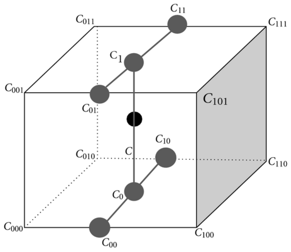
2.1.2. Algorithmic Details: Particle Advection

The efficient numerical treatment of particle advection is a relatively complex one as the critical path varies depending on many factors. We can simplify the problem and divide it into 5 major components:

• Data input/output (reading flow fields and writing particle coordinates to disk).
• Flow field interpolation (interpolate between simulation flow fields to “improve” temporal resolution for the integration scheme).
• Cell locator (finding where a particle is w.r.t. the original computational domain).
• Flow field velocity interpolation (calculating particle velocity based on its location within a cell).
• Particle movements (advancing particles forward, or backward, in time).

Each component stresses a different segment of a computational platform. For instance, I/O is very network-sensitive (in the case of a parallel file system), whereas velocity interpolation is very sensitive to both memory bandwidth and computational throughput (the precise balance is very dependent on the dataset due to cache effects). The cell locator portion is very interesting since it has been a major limiter in the past for many codes. Many authors have offloaded the cell locator to the CPU with a KD-Tree. Initially, we followed this approach, but it proved a major limiting factor for scalability. Moreover, porting a KD-Tree to the GPU was not the optimal choice. Ref. [28] implemented a hardware-accelerated solution leveraging Nvidia’s custom Bounding Volume Hierarchy structure in RTX GPUs. This solution, although efficient, is not vendor- or hardware-independent. For our solution, we drew inspiration from multi-grid methods in numerical linear algebra and efficient tree-traversal schemes. We apply a queue-less multi-level best-first search (QL-MLBFS). Let us expand on each term. The multi-level nature of our approach draws inspiration from multi-grid methods by introducing multiple coarser meshes. These coarser meshes are used to narrow down the location of a particle by “refining" only in the vicinity of a particle’s location. The coarsening factor is defined as $\lfloor {log}_2(N/2)\rfloor$, which enables efficient power-of-two mesh coarsening. However, GPUs have scarce memory pools and lack device-side global memory allocations. Therefore, we provide the illusion of mesh coarsening through strided memory views. On the device, each thread has a “view” of the global mesh focused on the current coarsening level and local neighborhood. To highlight the benefits of this multi-level approach, a mesh with dimensions $990\times 250\times 210$ (52 M nodes) will have a coarsening factor of 64, which leads to a top-level mesh of $14\times 2\times 2$ (56 nodes). This is a factor of 928,125×. The best-first search is directly inspired from the traditional BFS methodology, as illustrated by [29]. However, we exploit the structured spatial structure to remove the typical priority queue in the original BFS method. Coupling the two approaches and leveraging knowledge of the underlying structured mesh enables highly efficient cell locators. For a 52M node mesh, only 440 node evaluations are required, a factor of 118,125× less than brute-force search. A naïve octree would require ∼512 comparisons in the worst case (∼64 in the best case). We achieve comparable efficiency for a relatively large domain, with improved efficiency for smaller meshes. One very notable improvement is the lack of auxiliary data structures to hold the multiple levels. We highlight the pseudocode for our approach in Algorithm 1.

Algorithm 1 Multi-Level Best-First Search (ML-BFS)

$x_p,y_p,z_p$← Particle Coordinates $N_x,N_y,N_z$← Logical Dimensions $N\leftarrow min\left(N_x,N_y,N_z\right)$ $G\leftarrow \lfloor {log}_2(N/2)\rfloor$   ${\Delta }_c,{\Delta }_b\leftarrow$ Very Large Float (for example, ${10}^{38}$) $i,i_b,j,j_b,k,k_b\leftarrow G$   while   $i<N_x-G$   do     while $j<N_y-G$ do         while $k<N_z-G$ do            ${\Delta }_c\leftarrow \sqrt{{\left(x_{i,j,k}-x_p\right)}^2+{\left(y_{i,j,k}-y_p\right)}^2+{\left(z_{i,j,k}-z_p\right)}^2}$            if ${\Delta }_c<{\Delta }_b$ then                ${\Delta }_b,i_b,j_b,k_b\leftarrow {\Delta }_c,i,j,k$            end if            $k\leftarrow k+G/2$         end while         $j\leftarrow j+G/2$     end while     $i\leftarrow i+G/2$ end while   while   $G>1$   do     $i,j,k\leftarrow i_b-G,j_b-G,k_b-G$     while $i_b-G\le i<i_b+G$ do         while $j_b-G\le j<j_b+G$ do            while $k_b-G\le k<k_b+G$ do                ${\Delta }_c\leftarrow \sqrt{{\left(x_{i,j,k}-x_p\right)}^2+{\left(y_{i,j,k}-y_p\right)}^2+{\left(z_{i,j,k}-z_p\right)}^2}$                if ${\Delta }_c<{\Delta }_b$ then                    ${\Delta }_b,i_b,j_b,k_b\leftarrow {\Delta }_c,i,j,k$                end if                $k\leftarrow k+G/2$            end while            $j\leftarrow j+G/2$         end while         $i\leftarrow i+G/2$     end while     $G\leftarrow \lfloor G/2\rfloor$ end while

We can describe the scaling behavior of the proposed algorithm using the big-Oh notation. Big-Oh is a mathematical notation used to describe the asymptotic behavior of a function. It is often used in computer science and mathematics to describe the performance of algorithms and the complexity of problems. In general, big-Oh notation provides a way to compare the growth rates of different functions and to determine which functions grow faster than others as the input size increases. The scalable search algorithm for identifying the owning cell improves from the naïve $\mathcal{O}\left(N_p{N}_c^3\right)$ 3D search algorithm to a $\mathcal{O}\left(N_p{log}_8\left(N_c\right)\right)$. Given that $N_p$ (particle count) and $N_c$ (cell count) are uncoupled, we can theoretically approach the limit for $N_p>>{log}_8\left(N_c\right)$, which suggests a linear scaling in the number of particles. This is highly favorable considering that the naïve algorithm is $\mathcal{O}\left(N^4\right)$ for $\mathcal{O}\left(N_p\right)\approx \mathcal{O}\left(N_c\right)$.

Once the owning cell is identified, the particle’s velocity at an arbitrary natural coordinate n inside the owning cell is approximated using a trilinear interpolation scheme as follows:

$$U_n=c_0+c_1\Delta x+c_2\Delta y+c_3\Delta z+c_4\Delta x\Delta y+c_5\Delta y\Delta z+c_6\Delta x\Delta z+c_7\Delta x\Delta y\Delta z,$$

(3)

where the equation coefficients can be expressed in terms of the natural coordinates of the owning cell, where each dimension varies from $[0,1]$ (denoted by the subscripts, $xyz$, below). Hence, the coefficients are succinctly expressed as:

$$\begin{array}{cc}\hfill c_0& =U_{000}\hfill \\ \hfill c_1& =U_{100}-U_{000}\hfill \\ \hfill c_2& =U_{010}-U_{000}\hfill \\ \hfill c_3& =U_{001}-U_{000}\hfill \\ \hfill c_4& =U_{110}-U_{010}-U_{100}+U_{000}\hfill \\ \hfill c_5& =U_{011}-U_{001}-U_{010}+U_{000}\hfill \\ \hfill c_6& =U_{101}-U_{001}-U_{100}+U_{000}\hfill \\ \hfill c_7& =U_{111}-U_{011}-U_{101}-U_{110}+U_{100}+U_{001}+U_{010}-U_{000}\hfill \end{array}$$

The procedure is equivalent to performing 7 linear interpolations, as can be inferred from the diagram shown in [30] (faithfully reproduced in Figure 1 for convenience).

This is essentially a vector matrix product followed by a vector dot product; roughly 44 floating point operations on 3–14 data elements depending on cell coordinate/velocity reuse and counting the normalization of the cell coordinate. Arithmetic intensity is defined as a measure of floating point operations (FLOPs) performed with respect to the amount of memory accesses (bytes) needed to support those operations. The calculated variability in arithmetic intensity (i.e., 0.78–3.67 FLOPs per byte) highlights the significant uncertainty possible depending on the flow fields’ characteristics since many clustered particles could lead to a very high degree of data reuse, whereas a sparse placing of particles leads to low data reuse. For clustered particles, efficient memory access can lead to a mostly compute-bound interpolation kernel, whereas divergent particle trajectories can lead to a memory-bound kernel. This shows the vast complexities found in scientific computing workloads that are rarely described by simplistic categories and labels. On the contrary, the owning cell search algorithm is almost exclusively a memory-bound kernel. As such, the end-to-end kernel can morph from being memory-bandwidth-starved to being compute-bound and vice versa.

To avoid excessive floating point rounding errors when performing the interpolation step on small cells, we project all cells to a natural coordinate system regardless of their orientation or their volume. This ensures all interpolation is performed in the $[0,1]$ range (note the subindex for each term highlighting their natural coordinate within the unit cube), where floating point precision is greatest and limits excessive errors that would be introduced on small cells with the multiple calculations involved in the trilinear interpolation step ($\{\Delta x,\Delta y,\Delta z|\Delta x\in [0,1]\&\Delta y\in [0,1]\&\Delta z\in [0,1]\}$). To ensure stability when a particle is near (or at) the border of a skewed cell, $U_n$ is clipped to within the minimum and maximum velocities in the owning cell.

To mitigate memory requirements, we employed an explicit Euler integration scheme. Additionally, to further decrease storage demands, we incorporated the capability to interpolate between available flow fields using a first-order interpolation scheme. We evaluated higher-order interpolators, which offered negligible quality improvements over the first-order scheme. This outcome is likely due to several factors. Primarily, the timestep is sufficiently small, thereby minimizing the errors introduced by a first-order approximation and improving the stability and accuracy of the simulation [31]. We typically employ a timestep approximately 4–50× smaller than the DNS timestep, contingent on the computational cost and the desired quality. Secondly, the benefits of interpolation are predominantly found in the temporal upsampling potential of reducing the data loading requirements. If a low-resolution input is used, a higher-order scheme can introduce unphysical behavior between timesteps. Moreover, it is not straightforward to ensure that a generic high-order temporal interpolation scheme is bounded and conservative. Utilizing a small enough timestep and a linear scheme not only alleviates many of the concerns usually associated with these but also helps to preserve important conservation properties of the physical system being simulated [31]. Furthermore, it provides computational advantages due to reductions in data movements and higher arithmetic intensity relative to data transfers to/from the device [32,33] (discussed in further detail later in the paper).

The interpolation scheme invokes the following formulation:

$$u\left(t\right)=\frac{u_1-u_0}{t_1-t_0}\left(t-\frac{t_1+t_0}{2}\right)+\frac{u_1+u_0}{2}.$$

(4)

The interpolation scheme assumes a linear variation between two timesteps. A second-order approach implementation mostly generated similar results. By assuming linearity, we guarantee the results are bounded even when strong variations occur in a highly unsteady fluid flow. These strong variations are ubiquitous in high-speed, wall-bounded flow. Although more sophisticated interpolation and integration schemes exist, a simple yet highly efficient implementation has thus far yielded excellent results with strong computational scaling potential.

2.1.3. Algorithmic Details: Right Cauchy–Green Tensor and Eigenvalue Problem

One can quickly realize that the right Cauchy–Green (CG) strain tensor would require 9× more memory than the displacement field if the underlying software solution were to store each entry for every particle. This would quickly grow infeasible as the scaling would be linear in the number of particles with a large proportionality constant. Ideally, we would want the proportionality constant to be as close to unity as possible to ensure large-scale execution on limited memory platforms, such as the Nvidia Tesla P100 GPU, which is limited to 16 GBs. Furthermore, beyond merely an enabling quality, it is also a scalability requirement, allowing more particles on a single compute element. Our approach was to fuse the calculation of the right CG tensor and the eigenvalue calculation phase of the FTLE calculation. This requires only 36 to 72 bytes (depending on single or double precision requirements) of private memory per thread of execution, which often exceeds 100,000 threads of execution on a GPU and is just exceeding 50 to 60 on modern CPUs. For context, a V100 at maximum occupancy would require just 5.625–11.25 MiBs independent of the number of particles (2.3 to 4.6 KB on a 64 core CPU). This is in stark contrast to the 15–30 GBs that one of the large datasets presented herein (at large Reynolds numbers) would require (2538× higher memory requirements). Once the right CG tensor is calculated on an execution thread, the execution path proceeds to calculating the maximum eigenvalue for the given strain tensor. It is at this point where our CPU and GPU implementations diverge; library function calls are much more complicated on GPUs, which motivated our custom implementation of a relatively simple power iteration method [34]. The power iteration method is an iterative algorithm for finding the dominant eigenvalue and the corresponding eigenvector of a symmetric positive definite matrix of real numbers. The steps can be summarized as:

• Choose an initial guess for the eigenvector $x_0$ (preferably with unit length).
• Compute the product of the matrix A and the initial guess vector $x_0$ to obtain a new vector $x_1$.
• Normalize the new vector $x_1$ to obtain a new approximation for the eigenvector with unit length.
• Compute the ratio of the norm of the new approximation of the eigenvector and the norm of the previous approximation. If the ratio is less than a specified tolerance, then terminate the iteration and return the current approximation of the eigenvector as the dominant eigenvector. Otherwise, continue to the next step.
• Set the current approximation of the eigenvector to be the new approximation, and repeat steps 2–4 until the desired accuracy is achieved.

The power iteration method works well for symmetric positive definite matrices because these matrices have real and positive eigenvalues, and the eigenvectors corresponding to the dominant eigenvalues converge to a single eigenvector regardless of the initial guess. The rate of convergence of the power iteration method depends on the ratio of the largest eigenvalue to the second-largest eigenvalue and can be slow if the ratio is close to one. The power iteration is currently sufficient for our needs and computational budget; however, we are aware of more intricate methodologies that could be implemented if required, such as the QR algorithm.

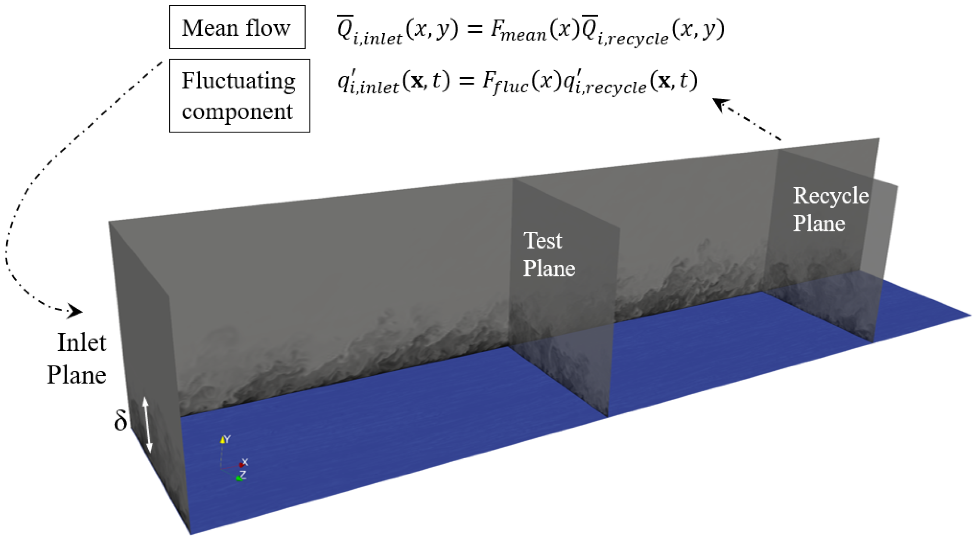
2.2. Direct Numerical Simulation: The Testbed Cases

This section describes the principal aspects of the testbed cases used for validation and assessment of the proposed particle advection methodology. Refs. [23,24,25] provide foundational background of presently employed DNS data based in terms of governing equations, boundary conditions, initialization, mesh suitability, resolution check, and validation. We are resolving spatially developing turbulent boundary layers (SDTBL) over flat plates (or zero-pressure gradient flow) and different flow regimes (incompressible, supersonic, and hypersonic). Particularly for incompressible SDTBLs, two very different Reynolds numbers are considered, the high-Reynolds case being about four times larger than its low-Reynolds-number case counterpart. The purpose is to examine the LCS code’s performance under distinct numbers of mesh points while somehow assessing Reynolds dependency on Lagrangian coherent structures. The employed DNS database in the present article was obtained via the inlet generation methodology proposed by [35]. The dynamic multi-scale approach (DMA) was recently extended to compressible SDTBL in [24,25] for DNS and LES approaches, respectively. It is a modified version of the rescaling–recycling technique by [36]. Extensions to compressible boundary layers have also been proposed by [37,38,39]. However, the present inflow generation technique does not use empirical correlations to connect the inlet friction velocity to the recycle friction velocity, as later described. A schematic of the supersonic computational domain is shown in Figure 2, where iso-contours of instantaneous static normalized temperature can be observed. The core idea of the rescaling–recycling method is to extract “on the fly” the flow solution (mean and fluctuating components of the velocity, temperature, and pressure fields for compressible flows) from a downstream plane (called “recycle”), to apply scaling laws (transformation), and to re-inject the transformed profiles at the inlet plane, as shown in Figure 2. The purpose of implementing scaling laws to the flow solution is to reduce the streamwise inhomogeneity of the flow. The Reynolds decomposition is implemented for instantaneous parameters, i.e., a time-averaged plus a fluctuating component:

$$u_i(\mathbf{x},t)=U_i(x,y)+u_i^{\prime }(\mathbf{x},t)$$

(5)

$$t(\mathbf{x},t)=T(x,y)+t^{\prime }(\mathbf{x},t)$$

(6)

$$p(\mathbf{x},t)=P(x,y)+p^{\prime }(\mathbf{x},t)$$

(7)

The re-scaling process of the flow parameters in the inner region [35] involves the knowledge of the ratio of the inlet friction velocity to the recycle friction velocity (i.e., $\lambda =u_{\tau ,inl}/u_{\tau ,rec}$). Here, the friction velocity is defined as $u_{\tau }$$=\sqrt{{\tau }_w/\rho }$, where ${\tau }_w$ is the wall shear stress and $\rho$ is the fluid density. Since the inlet boundary layer thickness, $\delta$, must be imposed according to the requested inlet Reynolds number, prescribing also the inlet friction velocity would be redundant. Refs. [36,37,38] solved this issue by making use of the well-known one-eighth power law that connects the friction velocity to the measured momentum thickness in zero-pressure gradient flows; thus, $u_{\tau ,inl}/u_{\tau ,rec}={({\delta }_{2,inl}/{\delta }_{2,rec})}^{-1/8}$. Since this empirical power (−1/8) was originally proposed for incompressible flat plates at high Reynolds numbers [40], it could be strongly affected by some compressibility effects and low to moderate Reynolds numbers, as in the cases considered here. Therefore, we calculated “on the fly” this power exponent, ${\gamma }_{\delta 2}$, by relating the mean flow solution from a new plane (the so-called “Test" plane, as shown in Figure 2) to the solution from the recycle plane as follows:

$${\gamma }_{\delta 2}=\frac{ln(u_{\tau ,test}/u_{\tau ,rec})}{ln({\delta }_{2,test}/{\delta }_{2,rec})}.$$

(8)

Table 1. DNS cases.

Case	${\mathit{M}}_{\mathit{\infty }}$	${\mathit{T}}_{\mathit{w}}/{\mathit{T}}_{\mathit{\infty }}$	${\mathbf{Re}}_{\mathit{\delta }2}$	${\mathit{\delta }}^{+}$	${\mathit{L}}_{\mathit{x}}$×${\mathit{L}}_{\mathit{y}}$×${\mathit{L}}_{\mathit{z}}$	$\mathbf{\Delta }{\mathit{x}}^{+}$,$\mathbf{\Delta }{\mathit{y}}_{\mathbf{min}}^{+}$/$\mathbf{\Delta }{\mathit{y}}_{\mathbf{max}}^{+}$, $\mathbf{\Delta }{\mathit{z}}^{+}$
Incomp. low	0	Isothermal	306–578	146–262	$45{\delta }_{inl}\times 3.5{\delta }_{inl}\times 4.3{\delta }_{inl}$	14.7, 0.2/13, 8
Incomp. high	0	Isothermal	2000–2400	752–928	$16{\delta }_{inl}\times 3{\delta }_{inl}\times 3{\delta }_{inl}$	11.5, 0.4/10, 10
Supersonic	2.86	2.74	3454–4032	840–994	$14.9{\delta }_{inl}\times 3{\delta }_{inl}\times 3{\delta }_{inl}$	12.7, 0.4/11, 12
Hypersonic	5	5.45	4107–4732	848–969	$15.2{\delta }_{inl}$ × 3 ${\delta }_{inl}$ × 3 ${\delta }_{inl}$	12, 0.4/12, 11

exhibits the characteristics of the evaluated four DNS databases of flat plates in the present LCS study: two incompressible cases (at low and high Reynolds numbers), a supersonic case ($M_{\infty }$ = 2.86), and a hypersonic case ($M_{\infty }$ = 5). Numerical details are reproduced here for readers’ convenience. The Mach number, normalized wall to freestream temperature ratio, Reynolds number range, computational domain dimensions in terms of the inlet boundary layer thickness ${\delta }_{inl}$ (where $L_x$, $L_y$, and $L_z$ represent the streamwise, wall-normal, and spanwise domain length, respectively), and mesh resolution in wall units ($\Delta x^{+}$, $\Delta y_{min}^{+}$/$\Delta y_{max}^{+}$, $\Delta z^{+}$) can be seen in Table 1. The momentum thickness Reynolds number is defined as $R{e}_{\delta 2}={\rho }_{\infty }{U}_{\infty }{\delta }_2/{\mu }_w$, and it was based on the compressible momentum integral thickness (${\delta }_2$), fluid density (${\rho }_{\infty }$), freestream velocity ($U_{\infty }$), and wall dynamic fluid viscosity (${\mu }_w$). On the other hand, the friction Reynolds number is denoted as ${\delta }^{+}={\rho }_w{u}_{\tau }\delta /{\mu }_w$. Here, $u_{\tau }=\sqrt{{\tau }_w/{\rho }_w}$ is the friction velocity, and ${\tau }_w$ is the wall shear stress. Subscripts ∞ and w denote quantities at the freestream and at the wall, respectively. Notice that the high-Reynolds-number case is approximately four times larger than that of the low-Reynolds-number case for incompressible flow.

For the low-Reynolds-number case (i.e., Incomp. low), the number of mesh points in the streamwise, wall-normal, and spanwise directions are 440 × 60 × 80 (roughly a 2.1-million point mesh). Whereas, the larger Reynolds number cases are composed by 990 × 250 × 210 grid point (roughly a 52-million point mesh). The small and large cases were run in 96 and 1200 processors, respectively, in the Cray XC40/50-Onyx supercomputer (ERDC, DoD), HPE SGI 8600-Gaffney, and HPE Cray EX-Narwhal machines (NAVY, DoD).

The present DNS databases were obtained by using a highly accurate, very efficient, and highly scalable CFD solver called PHASTA. The flow solver PHASTA is an open-source, parallel, hierarchic (2nd to 5th order accurate), adaptive, stabilized (finite-element) transient analysis tool for the solution of compressible [41] or incompressible flows [42]. PHASTA has been extensively validated in a suite of DNS under different external conditions [24,43,44]. In terms of boundary conditions, the classical no-slip condition is imposed at the wall for all velocity components. Adiabatic wall conditions were prescribed for both compressible cases. For the supersonic flow case at Mach 2.86, the ratio $T_w/T_{\infty }$ is 2.74 (in fact, quasi-adiabatic), where $T_w$ is the wall temperature and $T_{\infty }$ is the freestream temperature, while the $T_w/T_{\infty }$ ratio is 5.45 for the Mach 5 case. In the incompressible case, temperature is regarded as a passive scalar with isothermal wall condition. In all cases, the molecular Prandtl number is 0.72. The lateral boundary conditions are handled via periodicity, whereas freestream values are prescribed on the top surface. Figure 3 shows the streamwise development of the skin friction coefficient [$C_f$ = $2{(u_{\tau }/U_{\infty })}^2{\rho }_w/{\rho }_{\infty }$] of present DNS compressible flow data at Mach 2.86 and 5. It is worth highlighting the good agreement of present Mach-2.86 DNS data with experiments at similar wall thermal conditions, Reynolds, and Mach numbers from [45], exhibiting a similar slope trend in $C_f$ as a function of $R{e}_{\delta 2}$. An inlet “non-physical” developing section can be seen in the $C_f$ profile, which extends for barely 2.5-3${\delta }_{inl}$’s, indicating the good performance of the turbulent inflow generation method employed. Moreover, the inflow quality assessment performed in [23] via the analysis of spanwise energy spectra of streamwise velocity fluctuation profiles (i.e., $E_{uu}$) at multiple inlet streamwise locations and at $y^{+}=1,15$ and 150 indicated a minimal development region of 1${\delta }_{inl}$ based on $E_{uu}$. In addition, skin friction coefficient experimental data by [46,47] as well as DNS value from [48] at Mach numbers of 4.5 and 4.9 over adiabatic flat plates were also included. It is observed a high level of agreement with present hypersonic DNS results, and maximum discrepancies were computed to be within 5%. Furthermore, DNS data from [49] are also added at Mach numbers of 3 and 4 but at much lower Reynolds numbers.

Figure 4 shows the pre-multiplied energy spectra along the (a) streamwise ($k_x{E}_{uu}$) and (b) spanwise ($k_z{E}_{uu}$) directions in inner units at a Mach number of 2.86 at ${\delta }^{+}$ = 909. The supplied information by pre-multiplied energy spectra can be used to determine the streamwise and spanwise wavelengths of the most energetic coherent structures at different boundary layer regions. In both directions, primary energy peaks are evident in the buffer region around $12<y^{+}<15$ (see white crosses encircled by blue dashed lines), which are associated with spanwise wavelengths of the order of 100 wall units (or 0.1$\delta$) and streamwise wavelengths of the order of 700 wall units. This inner peak at ${\lambda }_x^{+}\approx$ 700 (or 0.7$\delta$) is the energetic “footprint” due to the viscous-scaled near-wall structure of elongated high- and low-speed regions, according to [50]. As expected, the turbulent structures associated with streamwise velocity fluctuations are significantly longer in the streamwise direction, showing an oblong shape with an aspect ratio of roughly 7. Furthermore, it is possible to observe weak but still noticeable secondary peaks with spanwise wavelengths of the order of ${\lambda }_z^{+}\approx$ 600 (or ${\lambda }_z\approx$ 0.7$\delta$) and streamwise wavelengths with ${\lambda }_x^{+}\approx$ 3000 (or 3$\delta$’s). These outer peaks of energy are much less pronounced than the inner peaks due to the absence of streamwise pressure gradient (zero-pressure gradient flow) and the moderate Reynolds numbers modeled. Present spanwise pre-multiplied power spectra, $k_z{E}_{uu}$, as indicated in Figure 4b, show a high similarity (including some “oscillations” of contour lines due to the high Reynolds number resolved), with pre-multiplied spanwise energy spectra of streamwise velocity fluctuations from [51] in their Figure 2b at $R{e}_{\tau }$ = 1116 (also known as ${\delta }^{+}$). They also performed DNS of a spatially developing turbulent boundary layer at the supersonic regime (Mach 2). It was also reported in [51] a secondary peak associated with spanwise wavelengths of ${\lambda }_z\approx$ 0.8$\delta$. According to [51], the outer secondary peaks are the manifestation of the large scale motions in the logarithmic region of the boundary layer, whose signature on the inner region is noticeable under the form of low wavenumber energy “drainage” towards the wall.

Figure 5 depicts the mean streamwise velocity by means of the Van Driest transformation ($U_{VD}^{+}$) and the streamwise component of the Reynolds normal stresses ${\left(u^{\prime }{u}^{\prime }\right)}^{+}$ in wall units. Additionally, three different logarithmic laws of $U_{VD}^{+}$ have been included. For these high values of ${\delta }^{+}$, the log region extends significantly (about 380 wall units in length). It seems our predicted values of $U_{VD}^{+}$ slightly better overlap with the logarithmic function $1/0.41ln\left(y^{+}\right)+5$ as proposed by [52] by the end of the log region (and beginning of the wake region). On the other hand, the log law as proposed by [53] (with a $\kappa$ value of 0.38 and an integration constant, C, of 4.1) exhibits an excellent match with our DNS results in the buffer region (i.e., around $y^{+}\approx$ 20–30). The inner peak of ${\left(u^{\prime }{u}^{\prime }\right)}^{+}$ occurs at approximately $y^{+}=15$ and an outer “hump” can be detected for the supersonic case at roughly $y^{+}=200-300$, consistent with the presence of the outer peak of the pre-multiplied spanwise energy spectra of streamwise velocity fluctuations.

2.3. Computing Resources

We leveraged a wide range of computational architectures and networks to test the performance portability and scalability of our proposed solution. The computational resources included Onyx, Narwhal, Anvil, and Chameleon.

2.3.1. Cray XC40/50-Onyx

Onyx utilizes a Dragonfly topology on Cray Aries and is powered by Intel E5-2699v4 Broadwell CPUs, Intel 7230 Knights Landing CPUs, and Nvidia P100 GPUs. The compute nodes are designed with dual sockets, each containing 22 cores, and are enabled with simultaneous multithreading (branded as Intel Hyperthreading). This allows the hardware threads to switch contexts at the hardware level by sharing pipeline resources and duplicating register files on both the front end and back end. The compute nodes are equipped with 128 GB of RAM, with 121 GB being accessible.

2.3.2. HPE Cray EX (Formerly Cray Shasta): Narwhal

Narwhal is a supercomputer capable of processing up to 12.8 petaflops. Each compute node on Narwhal contains two AMD EPYC 7H12 liquid-cooled CPUs based on the Zen 2 core architecture, with 128 cores and 256 threads, as well as 256 GB of DDR4 memory. There are a total of 2150 regular compute nodes on Narwhal, and the maximum allocation size is limited to 256 nodes. Additionally, there are 32 nodes with a single V100 GPU, and 32 nodes with dual V100 GPUs. The compute nodes are connected to each other using an HPE Slingshot 200 Gbit/s network, which directly links the parallel file systems (PFS).

2.3.3. Anvil

We also conducted a smaller-scale study using the CPU partition of the Anvil system at Purdue University. Built in collaboration with Dell EMC and Intel, it is designed to support a wide range of scientific and engineering research applications. The supercomputer is based on the Dell EMC PowerEdge C6420 server platform and is powered by the second-generation Intel Xeon Scalable processors. Anvil has a total of 1008 compute nodes, each containing 48 cores and 192 GB of memory. The nodes are interconnected with a high-speed Intel Omni-Path network that provides a maximum bandwidth of 100 Gbps. Anvil is also equipped with 56 Nvidia V100 GPUs for accelerating scientific simulations and deep learning workloads. Details on the Anvil system were well summarized by [54].

2.3.4. Chameleon A100 Node

We also tested scaling on more modern A100 GPUs provided by the Chameleon infrastructure [55]. The A100 node used features 2 Intel Xeon Platinum 8380 totaling 80 cores (160 threads) and 4 A100 GPUs with 80 GBs of HBM 2e memory. The node also has 512 GBs of DDR4 memory and 1.92 TBs of local NVMe storage.

2.3.5. Fair CPU and GPU Comparisons

Comparing CPUs and GPUs can quite easily become a misguided venture if not carefully guided by factual evidence and architectural distinctions. Although an in-depth comparison of CPU and GPU hardware is far beyond the scope of this work, we will summarize key distinctions between a general CPU architecture and a general GPU architecture. We will also establish the common ground between CPU and GPU architecture elements to be used in our comparisons.

CPU architectures have historically pursued low latency of an individual operation thread as their main goal. On the other hand, GPU devices favor high throughput by sacrificing the latency of an individual execution thread to enable processing a larger number of work items. GPU vendors tend to market ALU count (or SIMD FP32 vector lanes) as the “core count” for a device; however, this is misleading as the actual architecture unit resembling a “core” in a CPU device would be what Nvidia notes as a Streaming Multiprocessor (SM) (AMD tends to refer to this unit as a Workgroup Processor (WGP) or a Compute Unit (CU), whereas Intel refers to it as a X^e-core or a slice/subslice in older integrated GPU generations). To sustain a larger number of work items in flight, a GPU features a larger global memory bus width and typically has higher bandwidth requirements. Comparing the “per core” memory bandwidths shown in

Table 2. Computational device descriptions.

Device Name	P100 GPU (16 GB PCIe)	V100 GPU (32 GB PCIe)	A100 GPU (80 GB PCIe)	Intel Xeon E5-2699v4	AMD EPYC 7H12	AMD EPYC 7763
Core (SM) Count	56	80	108	22	64	64
FP32 Vector Lanes (VL)	3584	5120	6912	352	1024	1024
Global Mem. Bandwidth [GB/s]	732.2	897.0	1935	76.8	204.8	204.8
Mem. Bandwidth per Core [GB/s]	13.075	11.2125	17.917	3.49	3.2	3.2
Mem. Bandwidth per VL [MB/s]	204	175	280	218	200	200
Shared Cache [KB]	4096	6144	40,960	55,000	256,000	256,000
Shared Cache Bandwidth [GB/s]	1624	2155	4956	[56]	[57]	N.P.
Base Frequency [GHz]	1.190	1.230	0.765	2.2	2.6	2.45
Boost Frequency [GHz]	1.329	1.380	1.410	3.6 (SC) 2.8 (AC)	3.3 (SC) All-core N.P.	3.5 (SC) All-core N.P.
Est. TFLOPs/s Range [Min, Max]	8.529 9.526	12.595 14.131	9.473 17.461	1.548 Variable	5.324 Variable	5.017 Variable

, one could erroneously assume large advantage of modern GPUs over contemporaneous CPUs. Notwithstanding, upon closer examination and accounting for vector widths in each device, a smaller gap is seen, with the V100 actually having the lowest memory bandwidth per vector lane. Further complicating matters, shared cache bandwidth is a complex topic since it is often tied to core and fabric clockspeeds. These and other aspects are studied in further detail by [56,57]. Once again, this is not the whole picture. Accounting for register file sizes, one can note that modern GPUs boast zero-overhead context switching between multiple threads of execution, whereas modern ×86 CPUs have at most two sets of hardware registers, allowing for zero-overhead context switching between two threads of executions. This factor allows a large number of threads in flights in modern GPUs, which explains their resilience to high-latency memory operations regardless of their roughly equal memory bandwidth per vector lane. This architectural advantage is often the differentiating factor at scale for a throughput-oriented device as a GPU. Furthermore, the programming models supported by GPUs expose the parallelism supported by the device transparently, whereas historical high-level languages used in CPU programming are challenging when it comes to fully utilizing multi-core CPUs, their SIMD units, and available instruction-level parallelism. All of these factors typically compound and yield simpler, yet faster, code on GPUs even when devices are comparable on many fronts. A high-level overview of the computational devices used in this work is presented in Table 2.

2.3.6. Software

We implemented the proposed approach using Python as a high-level implementation language. However, achieving high performance and targeting multi-core CPUs and GPUs using plain Python is not possible at the moment. To achieve high performance on numerical codes, many libraries have been published targeting the scientific programming community. Perhaps the most popular numerical library for Python, NumPy by [58], provides a multi-dimensional array and additional functionality that enables near-native performance by targeting pre-compiled loops at the array level. Another relatively recent innovation in the Python ecosystem is the Numba JIT compiler by [59]. Numba enables compiling Python to machine code and achieves speeds typically only attainable by lower-level compiled languages, such as C, C++ or FORTRAN. Numba has been used across many scientific domains as both a tool to accelerate codebases and as a platform for computational research, as puth forth by authors such as [60,61,62,63,64,65,66,67,68,69,70,71,72,73,74]. Numba is essentially a front end to LLVM, which was originally proposed as a high-performance compiler infrastructure by [75]. Numba offers both CPU and GPU programming capabilities, which facilitates sharing components not tied to specific programming model details.

Numba’s parallel CPU backend also provides a higher level of abstraction over multiple threading backends. In particular, it allows for fine grain selection between OpenMP [76] and TBB [77]. Given the lack of uniformity in Lagrangian workloads after multiple timesteps, TBB’s ability to dynamically balance workloads while accounting for locality and affinity offers higher performance for our particular use case. That being said, the implementation can be changed by setting a command line argument at program launch. Moreover, with more exotic architectures featuring hybrid core designs or where certain execution resources can boost higher than others, TBB removes two issues with many parallel systems limiting scaling in heterogeneous systems, unbalanced workload, or large core counts: (1) it does not have a central queue, thus removing that bottleneck, and (2) it enables workers to steal work from the back of other workers’ queue.

3. Results and Discussion

In this section, we will drill in on the scaling behavior for the presented algorithm and implementation for particle advection. We will compare the performance across both CPUs and GPUs. We will also explore different normalization schemes to provide a fair comparison between these architectures. We will also explore the impact of a network-accessed parallel file system contrasted against a local high-performance NVMe device.

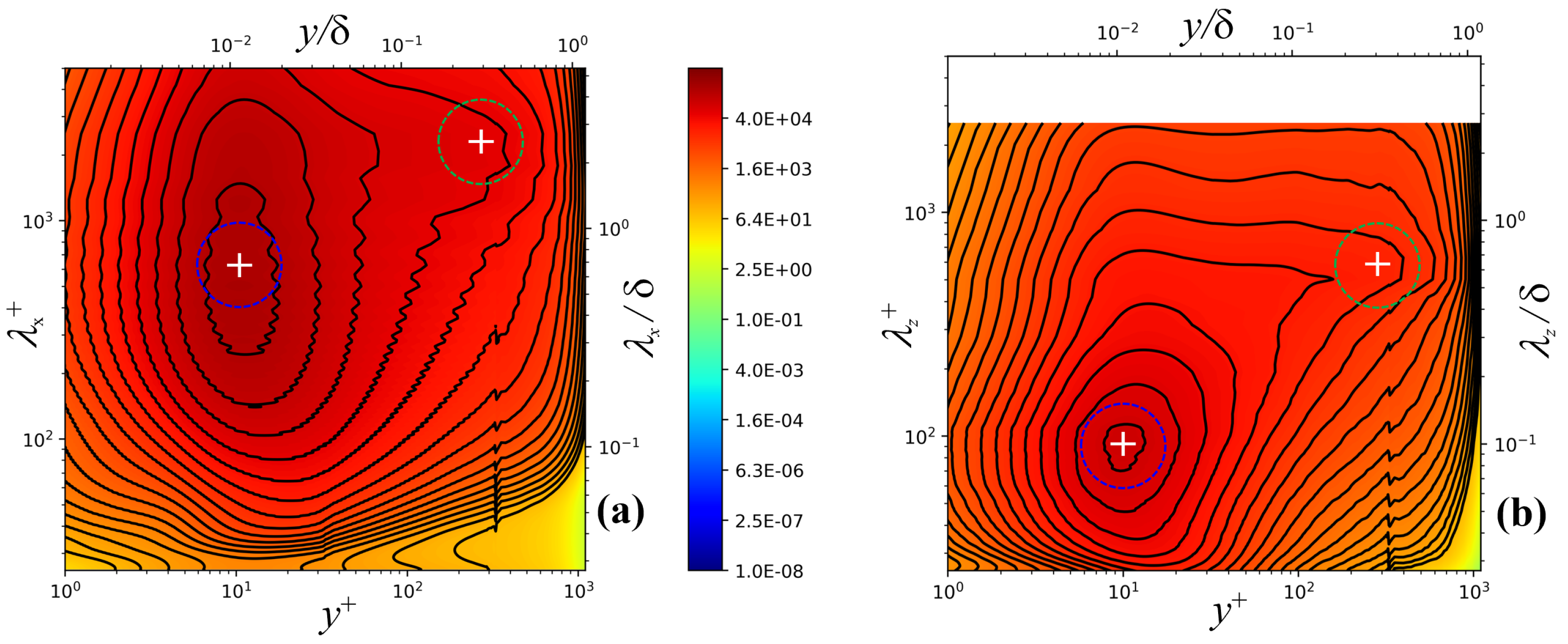
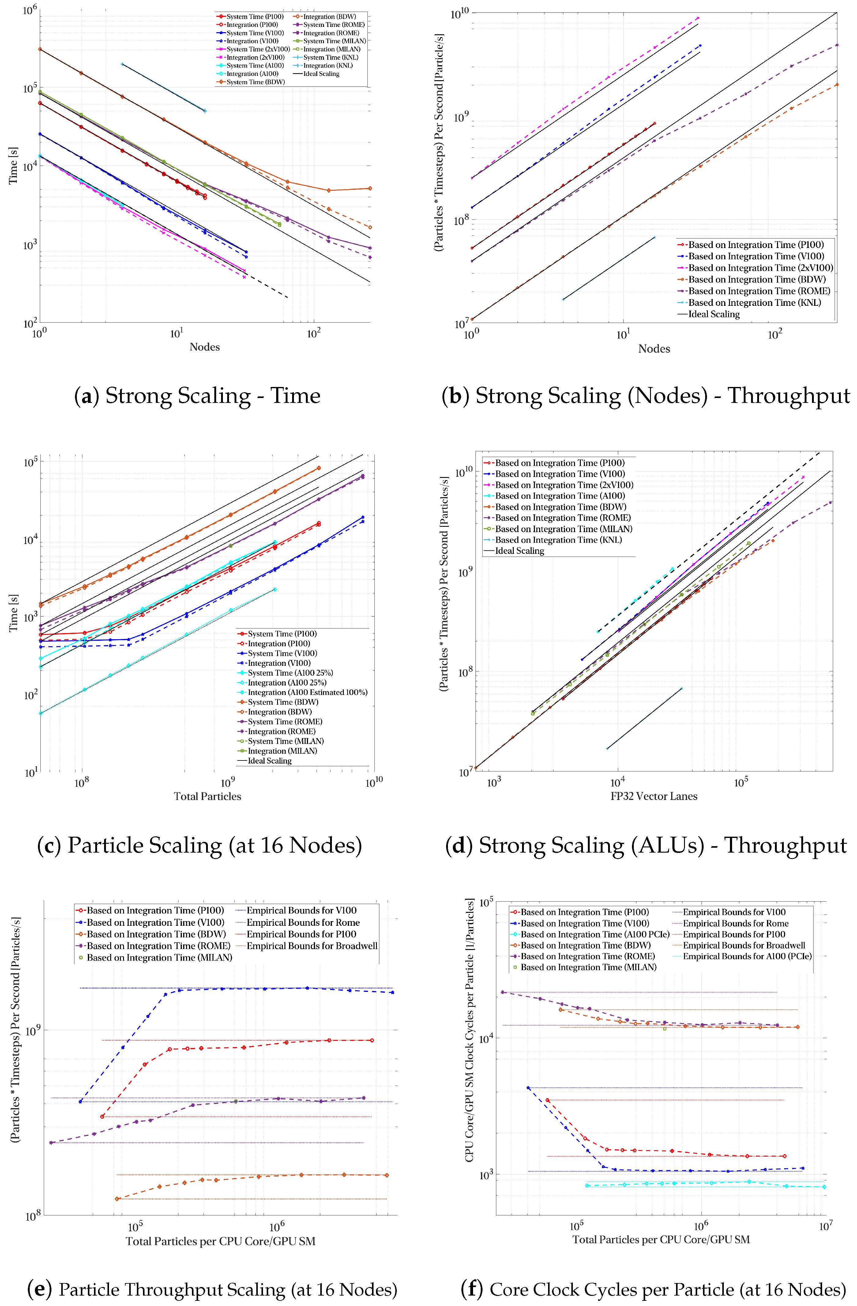
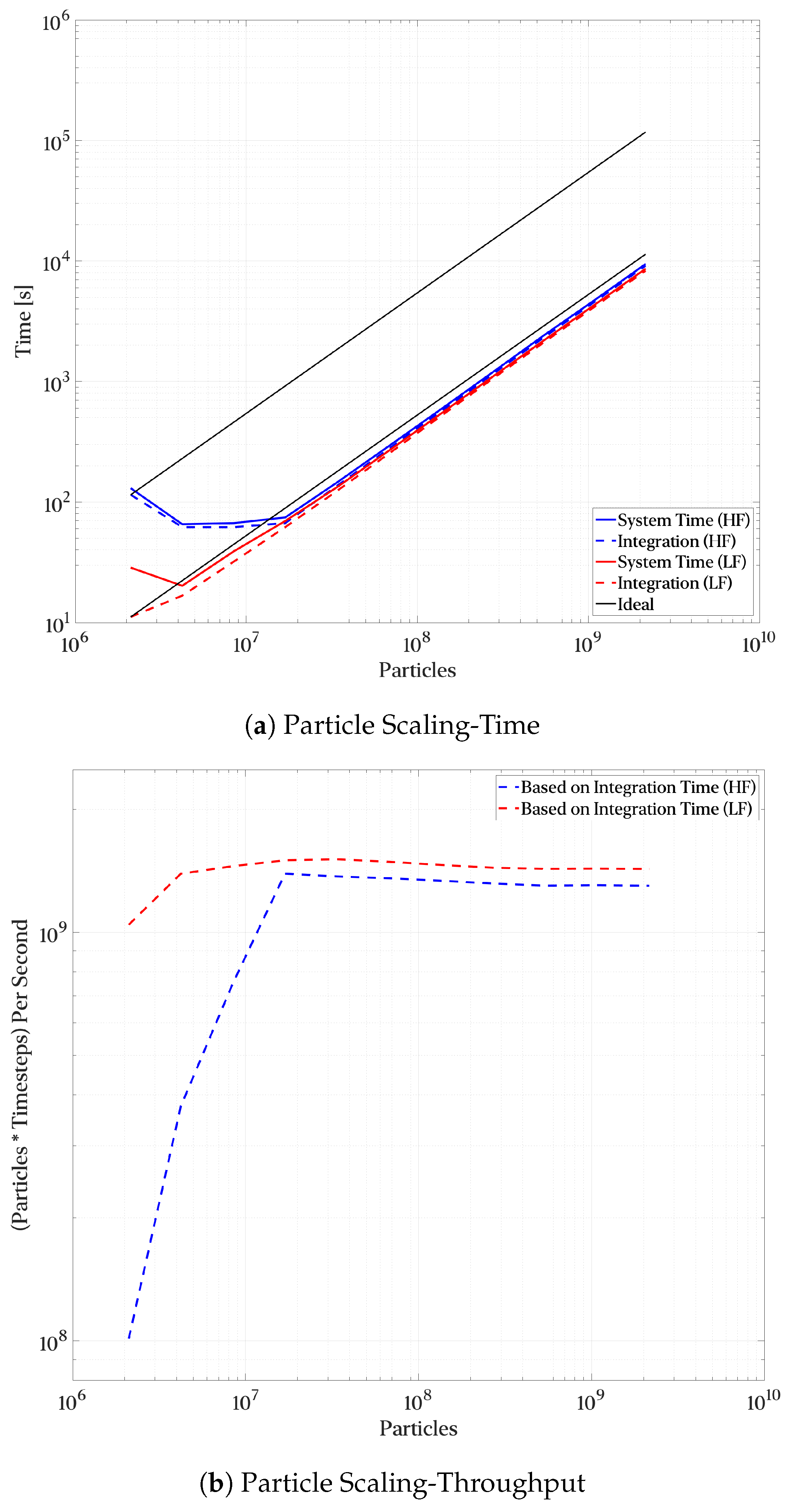
3.1. Performance Scaling Analysis

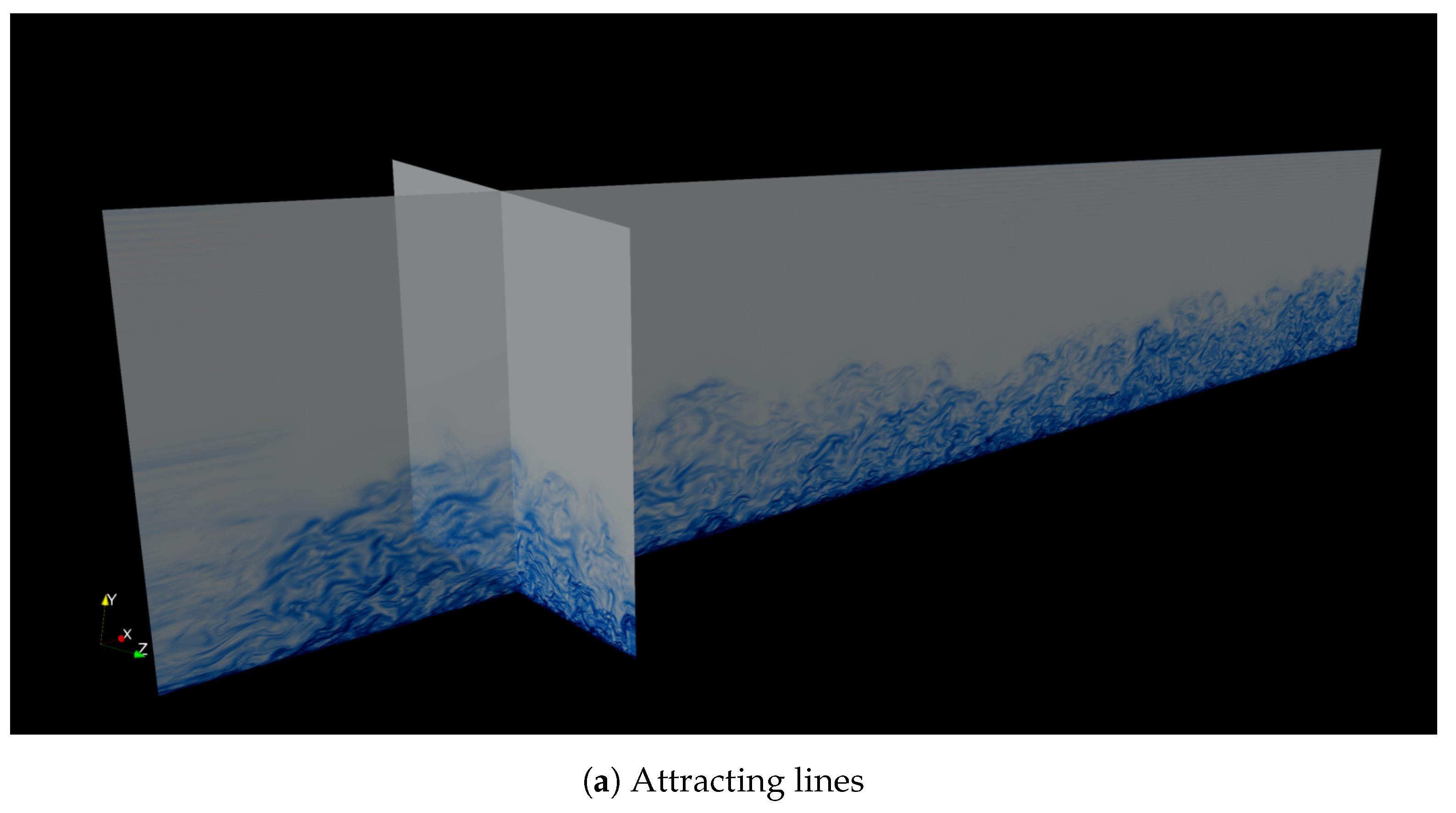
To begin our high-level exploration, we present multiple scaling plots in Figure 6. To efficiently utilize HPC resources, it is critical to scale out efficiently (i.e., to minimize serial bottlenecks). Figure 6a,b showcases the strong scaling performance of the approach put forth in this work. We scaled out to 32,768 CPU cores and up to 62 Nvidia V100 GPUs (4960 GPU SM cores or an equivalent 317,440 CUDA cores); consequently, the total number of CPU threads tested were roughly 32K, whereas the peak number of GPU threads reached roughly 10M (GPU) threads (2048 threads per Volta SM core arranged in blocks of 64 threads for a total of 32 thread blocks per SM), or 310× more threads on a GPU (GPU threads are lightweight threads compared to the heavier OS-managed threads on CPUs). Figure 6a also highlights the extent that inefficiencies in the software stack or hardware resources below the application can end up degrading the performance at scale. This is clearly visible in Onyx, where a large number of IO/network requests dominate the startup/termination times of the application, and actual runtime scales almost linearly. Beyond the impact of having a linear strong scaling behavior, scaling to large particle count is an equally important aspect as larger datasets and more challenging scientific inquiries demand higher resolutions. Figure 6c characterizes the scaling behavior of our implementation on a fixed node count (i.e., fixed computational resources) from 50 M particles out to over 8 B particles (given enough memory was available) across 16 compute nodes. One other interesting tidbit worth highlighting is the dominance of network latency in large-scale parallel file systems (PFS). Figure 6c showcases how a powerful GPU is essentially idle when waiting for data from the PFS (for both the P100 and V100 results). Ref. [63] reported a similar behavior for small problem sizes on a parameter estimation workload. Interestingly, they reported this behavior up to a 9 M element matrix (3000 × 3000), whereas we found the onset of this behavior at approximately 13 M particles. Consequently, a good rule of thumb is roughly 10 M work elements per GPU. This is the incarnation of Amdahl’s law, where the GPU is essentially acting as an infinitely fast processor where the critical path lies on IO, sequential routines, the network, and the PFS. This is further confirmed by the A100 results, where data resided on a local NVMe drive. Once sufficient work is available, the pre-fetch mechanism first introduced in [18,19] is capable of hiding the latency to great effect. In general, our proposed approach is very scalable in both particle count and strong scaling via problem decomposition. As processors continue to improve, multi-level approaches and latency-hiding mechanisms will continue growing in relevance to fully utilize the available computational resources.

Recall that we outlined in Section 2.1.2 the computational complexity scaling for the particle tracking algorithm in terms of cell count and particle count. For a large number of particles $N_p$ and cells $N_c$, the term $N_p{log}_8\left(N_c\right)$ can be approximately modeled as linear scaling in $N_p$. This is because, as $N_c$ increases, the growth rate of ${log}_8\left(N_c\right)$ is much slower compared to the linear growth of $N_p$. As a result, the overall function appears to scale linearly with $N_p$, even though there is a logarithmic dependence on $N_c$. This favorable scaling will prove very powerful as larger datasets are tackled and to enable higher-resolution LCS visualizations in smaller datasets. What is more, by using $N_p>>N_c$, the overall particle advection scheme is mostly dominated by velocity interpolation and temporal integration (source of the $N_p$ term) rather than by volumetric particle search (source of the ${log}_8\left(N_c\right)$ term). Moreover, for any given domain, increasing the particle count results in a linear increase in the number of particles due to the decoupled scaling characteristics of the algorithm on the size of the domain and particle count. This conclusion is clearly shown in Figure 6c, where, once fixed latency costs are hidden by the pre-fetcher, a linear scaling is indeed observed. As will be discussed later in the article, we tested our implementation against a 24.6× smaller DNS dataset to validate the favorable scaling in the number of cells. Although the high-Re dataset used in this work is almost 25× larger than the lower-Re counterpart, the overall runtime is only 41% higher when accounting for particle count differences and flow field count differences to achieve similar integration $t^{+}$ and particle count. That is a mere 15% difference of what is predicted from the big-Oh analysis. That 15% is attributable to inefficiencies reading 45% more flow fields (we accounted for this in calculating the comparison, but, given that the network is involved, differences are to be expected in addition to many other factors) and other factors unaccounted in our big-Oh approximations.

We will discuss in more detail the architectural advantages in relation to the results below, but an initial overview of the remaining scaling results in Figure 6 highlights the virtues of an architecture built fundamentally for throughput and explicit parallelism. Each GPU SM offers higher per-clock throughput, which translates to a palpable advantage on embarrassingly parallel workloads. On the other hand, CPUs can also take advantage of parallel workloads. As such, explicitly developing parallel algorithms enables improved performance rather than porting an implicitly parallel workload to an explicitly parallel device. However, Figure 6d also highlights the dangers of naïvely comparing CPUs and GPUs without accounting for their architectural similarities and differences. Figure 6d shows the same results presented in Figure 6b but scales the horizontal axis to account for SIMD vector lanes in both CPUs and GPUs. After this linear transformation, the overall performance advantage of GPUs (still present) is not as abysmal as in Figure 6a,b. This smaller gap accentuates the convergence of CPUs and GPUs towards ever more similar design elements. SIMD units in CPUs are akin to CUDA cores in Nvidia GPUs, albeit with slightly different limitations and programming models. Nonetheless, they serve the same purpose, applying the same instructions (more or less) to multiple data streams. As such, formulating algorithms to reduce synchronization or serialization points enables a more transparent scaling potential as more parallelism becomes available in future hardware.

Figure 6e shows the particle throughput per timestep over 16 nodes. As was alluded to in the discussion, once sufficient work is available, the throughput stabilizes to a plateau. Of the devices used to study the particle throughput and the performance scaling, the GPU accelerators achieve the highest throughput as compared to available CPU devices. A single V100 GPU achieves a throughput of 105M particles per second (1.7B particles per second over 16 V100 GPUs; 1.3M particles per GPU SM). Comparatively, 32 EPYC 7H12 CPUs (2048 cores) achieve a total throughput a 426M particles per second (13M particles per second per 7H12 socket; 203K particles per second per Zen 2 core). Without accounting for clockspeeds, the overall throughput of a Volta SM core is 6.4× a Zen 2 core. Upon accounting for clockspeeds (as shown in Figure 6f), the clock for clock performance of a GPU SM is still greater than that of a CPU core. Interestingly, the improvements across both CPU and GPU generations are much more incremental than revolutionary according to the SM count and clockspeeds in Figure 6f. However, given the magnitudes of modern processor clockspeeds, a single V100 GPU can process a particle in roughly 9.8 ns (in parallel to many other particles); however, analyzing a single SM yields roughly 900 ns. We could continue to modify the results to analyze the per SIMD partition performance yielding the “worst” results. Consequently, application developers ought to be careful when presenting scaling data and avoid implicit biases against a (or in favor of) given vendor.

Thus far, we have focused our discussion on a single relatively large DNS simulation. However, smaller-scale simulations deserve special attention due to peculiarities pertaining to their latency-sensitive nature during post-processing. To investigate this issue, we ran the same particle advection workload across a series of lower-$Re$ DNS flow fields on 16 Nvidia V100 GPUs. The sensitivity to network IO was isolated by introducing two underlying DNS sampling frequencies. The high-frequency (HF) samples were stored at the DNS timestep resolution and internally interpolated to achieve a timestep 50× smaller than the DNS timestep. Conversely, the lower-frequency (LF) sample was sampled at a tenth of the DNS resolution with a 500× upsample via interpolation applied to achieve an equal integration timestep. The physical implications of these two approaches will be discussed in Section 3.2.3. Due to the lower amount of work at low particle counts, performance is actually worse at very low particle counts than for subsequent increases due to high data transfer overheads and synchronization penalties. By reducing the underlying number of actual flow fields and producing approximations inside the GPU via interpolation, we essentially cut data movements to just 10%, significantly improving the performance, as shown in Figure 7a. Analogous to what we discussed for Figure 6e, Figure 7b exhibits a similar plateau at just over 1.5 billion particles processed per second on each timestep. The data transfer overhead is still seen in both figures by the small difference in the asymptotic limit of both cases. The peak throughput for the LF case settles at 9% over the HF peak throughput owing to data transfer overhead. That being said, saturating the device and hiding transfer overheads can be achieved at a lower particle count than when a larger underlying flow field is being used. This can be justified noting the particle search approach being used where more data are being reused and cached in the multi-level scheme than for the higher-Re case. A single low-Re flow field occupies 25 MBs, whereas an equivalent field for the higher-Re case occupies 623 MBs (note that the L1+L2 cache capacity of a V100 comes in at approximately 16 MBs). The peak throughput for the low-Re case is achieved at roughly 16 M–32 M particles, whereas the high-Re case requires 500 M–2000 M particles (15–125× more than the lower-Re case). In general, achieving peak throughput requires at least an order of magnitude more particles than number of vertices in the underlying flow fields to allow the pre-fetcher enough slack to hide the network latency penalty when reading from the parallel file system. It ends up being a “free” resolution improvement, as noted in Figure 6e and Figure 7a, with a fixed runtime until the device is properly utilized.

Evaluating the particle advection approach and its performance portability requires testing across a wide variety of architectures. Historically, certain algorithms have been better suited for GPUs, whereas others are more efficient on CPUs. However, in recent times, CPUs and GPUs have continued to evolve into highly parallel architectures with many elements in common. Take, for instance, a relatively modern Nvidia GPU, the V100. The V100 has 80 SM cores (the architectural unit closest to a CPU core), with each core having four partitions with 3 × 512-bit SIMT units (one single precision floating point, one double precision floating point, and one integer SIMT unit per partition). A modern AMD server CPU such as 7H12 or 7763 both have 64 cores with 2 × 256-bit SIMD units, which equals the total length of the floating point pipeline on a single SM partition in the aforementioned V100 GPU (although four scalar integer ALUs are present in Zen 2/3, which, to be fair with our GPU comparison, leads to a 128-bit lane-width assuming 32-bit integer operations). Clock for clock, a GPU SM is capable of approximately 4–9.6× the computational throughput, ranging from raw FP32 throughput to a perfectly balanced (FP32 and FP64 float/integer) and scalable workload. That being said, a GPU SM has a far larger register file, enabling zero-overhead context-switching. This makes the GPU far more latency-tolerant. These factors enable a highly scalable programming model on GPUs, whereas achieving scalable throughput on CPUs requires much more finetuning. Accounting for clockspeeds and core counts, we should expect to see a speed-up of approximately 4.25× of a single Tesla V100 over an EPYC 7H12. We measured an empirical speed-up based on the strong scaling workload at 3.9× average (3.3× minimum and 5× maximum) or 92% of our theoretical estimate based on raw throughput, as shown in Figure 6e–f. It is worth noting that the simpler analysis of bandwidth and compute throughput suggested a less aggressive 2.3× to 2.7× performance improvement, which leaves another 57% improvement in algorithmic performance on the table without considering the combined integer/floating point throughput of modern architectures. This analysis would suggest the improvements of an A100 GPU are roughly 38–60% over a V100 GPU (from throughput to bandwidth improvements). Analyzing A100’s performance for our particle advection implementation showcases a 79% improvement when comparing a single V100 vs. a single A100 GPU (see Figure 6c). Out of this 79%, the additional SMs and higher clockspeeds yield a 38% improvement, whereas architectural enhancements contribute a 30% improvement. Clock for clock, we found the A100 to be 28% faster in our testing. These results are in line with the 60% “per-SM” memory bandwidth improvement and 35% increment in SM count. These additional bandwidth improvements are also “reachable” given the vastly improved cache in A100. The per FP32 lane performance is shown in Figure 6d, where CPU lanes are calculated based on the SIMD pipeline widths and GPU lanes are taken as the CUDA core count (Nvidia’s marketing term for FP32 ALU). The performance gap is significantly reduced when comparing against the FP32 vector lane count, which yields a fairer comparison point normalizing against the baseline throughput unit. However, we assess that algorithmic and implementation improvements could still yield another 20% improvement in achievable performance. A100 offers a vastly larger cache subsystem, unlike prior GPU generations, which likely necessitates finetuning. This highlights the importance of a multi-faceted analysis when evaluating potential performance improvements. Moreover, our particle advection codebase is highly scalable, with additional memory bandwidth and throughput. Given the ever-improving hardware landscape, our proposed implementation should be performance-portable across multiple hardware generations. Hence, we believe that domain experts should consider additional avenues of exploiting the concurrent execution of floating point and integer calculations given the potential doubling in throughput on modern architectures in addition to the more traditional improvements associated with memory bandwidth utilization.

We leverage the fact that modern CPU architectures in HPC systems continue to converge with GPUs and share a common approach (albeit implemented in different programming models). Algorithm 1 forms the foundation of our particle advection implementation on both CPU and GPU. As seen in Figure 6a,b, we achieve strong scaling across both CPU and GPU nodes and across various generations. We do observe a degradation in strong scaling performance at higher node counts for the Onyx and Narwhal systems when using CPU-only node configurations. We assess that this breakdown is a limitation of the file system rather than a limitation of the actual implementation. This is further reinforced by the results in the Anvil system. Although not shown, the system is capable of targeting both CPUs and GPUs in a hybrid approach through the same LLVM compiler infrastructure. This hybrid approach currently targets a static work scheduler and requires user-guided finetuning to estimate an appropriate work-sharing strategy. Looking towards possible optimization avenues, a more automated and dynamics approach would enable a fully automated backend that fully utilizes the available hardware.

The right CG tensor and the maximum eigenvalue calculation currently represent a minimal portion of the overall runtime. However, we measure the performance on a single P100 GPU at 204 K eigenvalues per second for a 415 M particle system, representing roughly 33 min to calculate the finite-time Lyapunov exponent for each particle from the displacement field (∼3% of the total runtime). A V100 offers a higher throughput for the eigenvalue solver and the integration scheme as shown above. It achieves 711 K eigenvalues per second for a 67 M particle system (representing roughly the same percentage of the total program runtime). The major limitation is the nature of the eigenvalue problem at hand, where we have to solve one small eigenvalue problem per particle. Many high-performance implementations are tuned for large sparse problems. Tuned batched implementations exist but require submitting the batched buffers as a whole. Given our trade-off between available memory footprint requirements and performance, our streaming approach is a sensible solution.

3.2. Case Study

To prove the applicability and usefulness of the proposed approach, we applied our methodology to three previously obtained DNS datasets [23] to assess the compressibility effects on Lagrangian coherent structures over moderately high Reynolds number turbulent boundary layers at three flow regimes, ranging from incompressible, supersonic, and hypersonic, as already described in Table 1. As discussed in [9], a time convergence analysis was performed at different integration times, i.e., at $t^{+}=$ 10, 20, and 40, where $t^{+}=u_{\tau }^{2}t/\nu$. More defined material lines were observed as the integration time was increased. Following [9], the results shown henceforth are based on a backward/forward integration finite time of $t^{+}=\pm 40$. Firstly, we showcase the ability to perform LCS analysis at scale (hundreds of millions to billions of particles). Figure 8, Figure 9 and Figure 10 show FTLE contours in incompressible, supersonic, and hypersonic regimes, respectively. Furthermore, isometric views are depicted for attracting manifolds (top) and repelling manifolds (bottom) by performing backward or forward integration of particle advection, respectively. The DNS mesh is composed of approximately 52 million grid points, whereas 416 million particles were evaluated in all cases. In Figure 8a, the incompressible attracting FTLEs depict the presence of hairpin vortices, consistent with results by [78,79]. Hairpin vortices have been broadly accepted as the building blocks of turbulent boundary layers [80]. Furthermore, one can observe that attracting LCS ridges (blue contours) reproduce inclined streaky structures with the upstream piece stretching towards the near-wall region, almost attached to it, while the downstream part is elongating into the outer region due to viscous mean shearing [9,79]. In other words, these lateral images of attracting FTLE manifolds depict inclined quasi-streamwise vortices (or hairpin legs) and heads of the spanwise vortex tube located in the outer region. In some streamwise locations, hairpin heads can rise up into the log or wake layer (not shown), i.e., 30 <$y^{+}$< 700, due to turbulent lift-up effects. In addition, hairpins are rarely found isolated but in groups or packets. Ref. [81] identified Lagrangian coherent structures via finite-time Lyapunov exponents in a flat-plate turbulent boundary layer from a two-dimensional velocity field obtained by time-resolved 2D PIV measurement. They stated that hairpin packets were formed through regeneration and self-organization mechanisms. There is a significant qualitative agreement between attracting lines of Figure 8a and the corresponding attracting lines computed by [78,79], as shown in their Figures 6 and 8, respectively. Moreover, Ref. [82] reported a high level of correlation between attracting FTLE manifolds and ejection events (or Q2 events) in supersonic turbulent boundary layers. As a hairpin vortex moves downstream, it generates an ejection of low-speed fluid (i.e., Q2 event), which encounters zones of higher-speed fluids, resulting in shear formation and, consequently, increased drag. Further, “kinks” can be observed in some hairpin vortex legs (attracting FTLE’s contours) due to viscous interaction within hairpin vortices. Repelling manifolds via forward temporal integration have also been computed and visualized in Figure 8b. Different from attracting material lines, repelling barriers are mostly concentrated in the very near-wall region. Notice the large values of repelling FTLEs (intense red) very close to the wall. However, they are also clearly observed in the buffer/log region with lower intensity, intersecting hairpin legs in regions where ejections are commonly present.

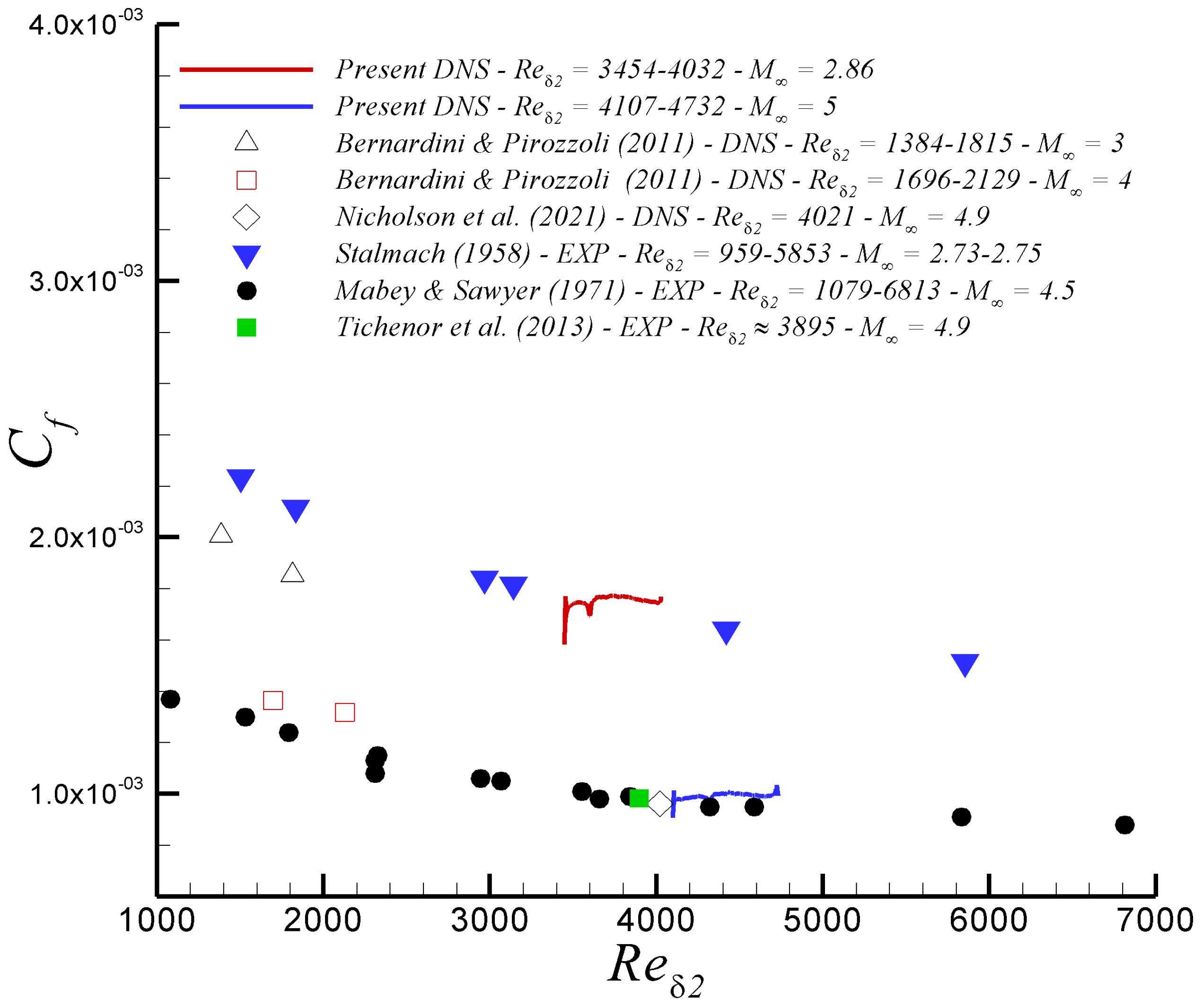
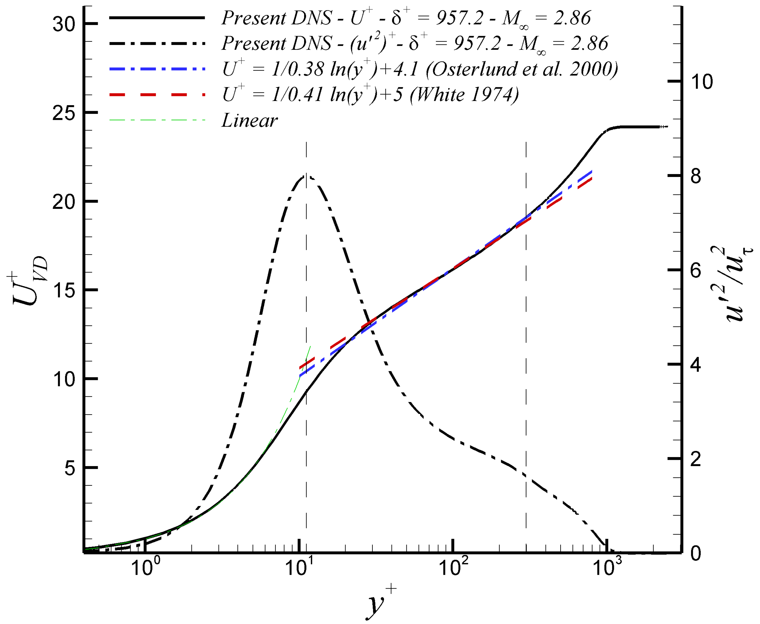
3.2.1. Compressibility Effects

The prior descriptions of features of attracting/repelling manifolds in incompressible turbulent boundary layers are fully extensible to supersonic and hypersonic flat-plate turbulent boundary layers. Two main compressibility effects can be highlighted: (i) coherent structures grow more isotropic proportional to the Mach number; (ii) the inclination angle of the structures also varies along the streamwise direction. The increased isotropic character is perhaps the most interesting of both. The incompressible coherent structures are relatively weak in nature and mostly confined to the near-wall region, with the presence of a more evident “valley” between “bulges”. This is in stark contrast with the hypersonic coherent structures and shear zones that are apparent farther from the wall. Conversely, the prevalence of the structures farther away from the wall does not convey the complexity of the phenomenon. Although these structures and shear layers are more prevalent farther from the wall, they seem much more isotropic (but less organized) and contained in smaller clusters. This effect has been reported in the past in Eulerian statistics by [3] and Lagrangian statistics by [9].

3.2.2. Reynolds Number Dependency Effects

Aside from the relatively moderate compressibility effects on LCS, we did observe a stronger dependency on the Reynolds number, as expected. The structures are far more anisotropic and organized at lower Reynolds numbers, as shown in Figure 11. Structures at lower Reynolds numbers extend significantly along the streamwise direction, whereas structures at higher Reynolds numbers tend to be shorter in general with smaller coherency spans. At lower Reynolds numbers, the presence of hairpin vortex packets (or horseshoes) is more evident. These are observable by grouped regions of high coherency in the attracting FTLE ridges.

The isometric view shown in Figure 12 illustrates that the increased coherency in the lower Reynolds case extends significantly in the spanwise direction as well. This also confirms the increased anisotropy. We hypothesize that the increased fluid organization at lower Reynolds numbers is attributable to a decreased dominance of the inertial forces. The viscous interactions offer a “stabilizing” effect on the coherent structures and elongate their coherency.

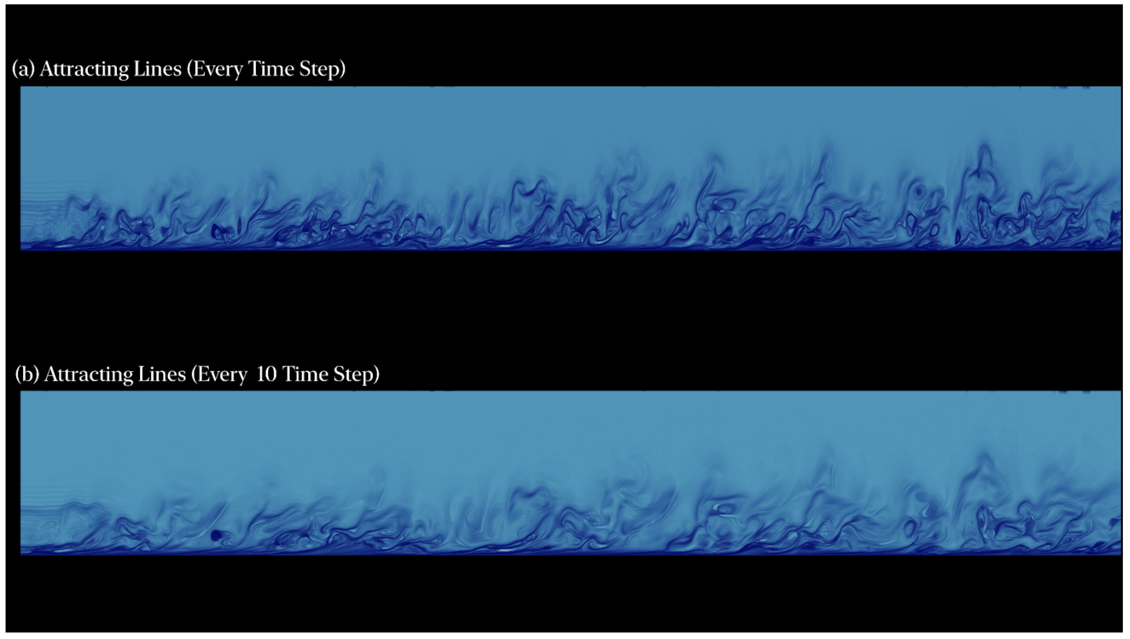
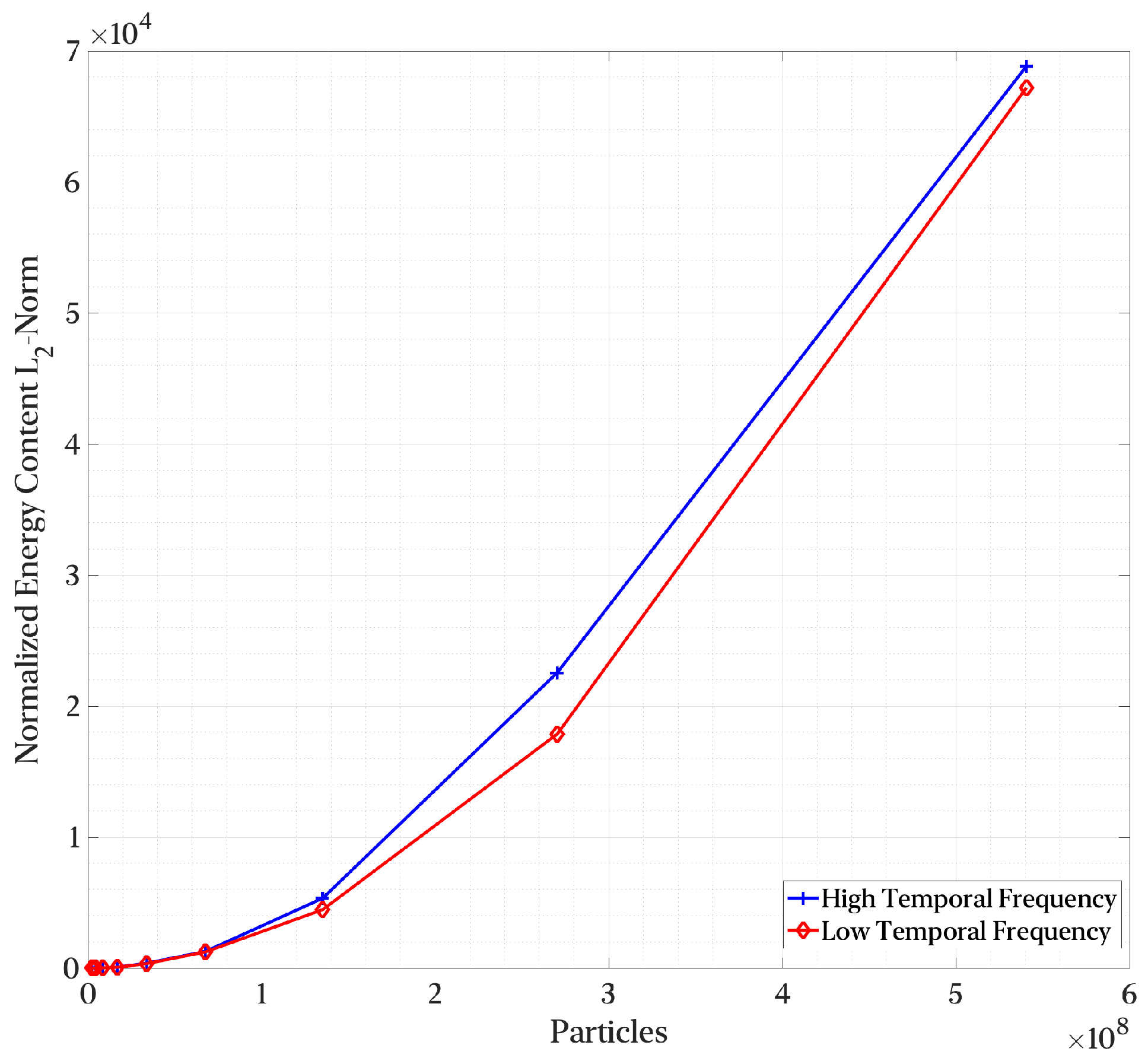
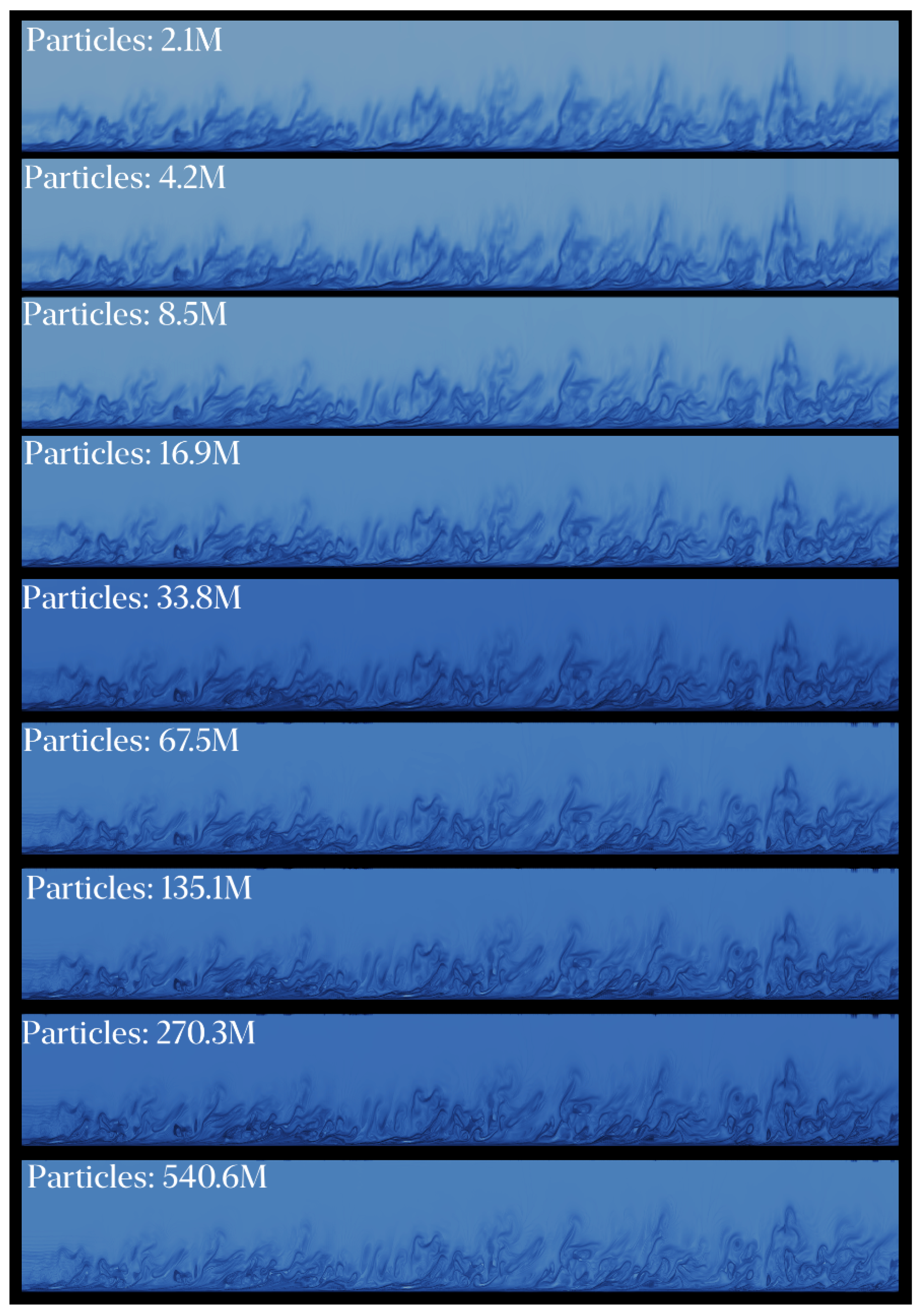
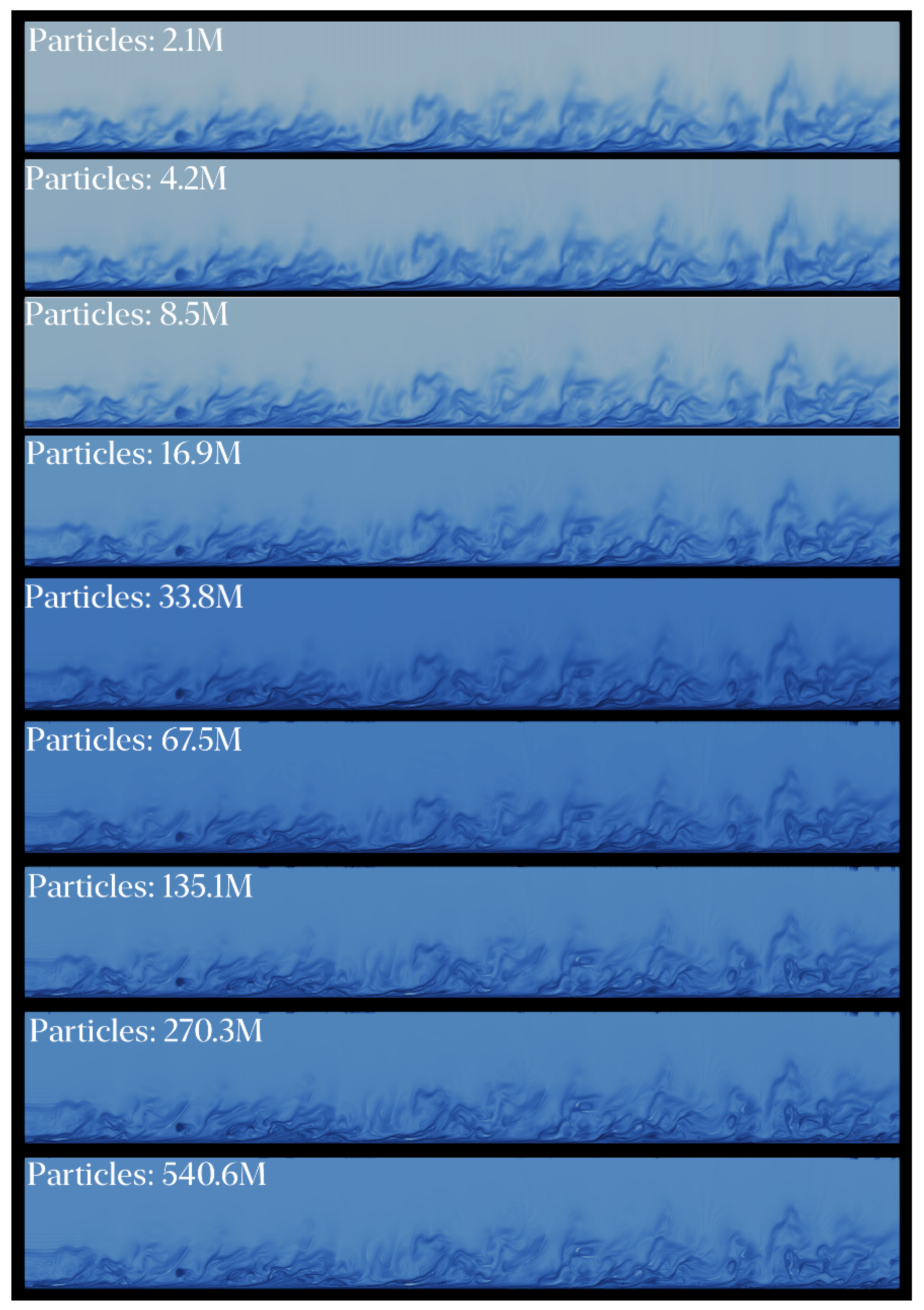
3.2.3. Temporal Interpolation and Particle Density Influence

The temporal interpolator presented in Equation (4) provides a mechanism to reduce storage requirements. To assess the quality of our interpolation mechanism, we showcase results sampled at different temporal resolutions (an order of magnitude difference) for the incompressible low-Reynolds-number case. The results are shown in Figure 13. Note that both particle advection integration tests (and using the proposed interpolation scheme) were executed at a timestep that was 20× smaller than that of the DNS timestep. In general, the structures are well preserved, with the only features slightly degraded containing high frequencies that inherently depend on high-frequency sampling, and the interpolation scheme preserves the stability of the integration process.

To validate the higher frequency features in our simulation, we put forth a hypothesis that, as the particle count increases and as the underlying flow fields are sampled at a higher rate, more “energy” or intensity is concentrated into the same volume. This concentration of energy results in the structures within the flow becoming more well-defined. This hypothesis is based on the fundamental principles of turbulence, where energy cascades from larger scales to smaller scales, and the smaller scales contain a higher frequency of fluctuations. To test our hypothesis, we employ an approach analogous to that of a power (energy) spectra to calculate the density of the finite-time Lyapunov exponent (FTLE) intensity. The FTLE is a measure of the rate of divergence or convergence of nearby trajectories in a flow field, and its intensity can provide insights into the structure and dynamics of the turbulence. In Figure 14, we present a normalized view of this spectral analysis. As anticipated, the FTLE’s intensity grows and is concentrated into smaller regions, which results in higher magnitudes in the $L_2$-norm of the spectra as the particle count increases and at higher temporal sampling frequencies. Interestingly, both curves follow almost a quadratic tendency. This trend can be visually confirmed by closely inspecting Figure 15 and Figure 16, although it is slightly more obfuscated. While increasing the temporal sampling frequency does yield more well-defined results, we also find that increasing the number of particles can lead to similarly high-fidelity results at higher particle counts. This suggests that the resolution of the simulation in both the spatial and temporal dimensions plays a crucial role in capturing the higher-frequency features of the turbulence. However, it is important to note that some features of the turbulence are inherently tied to the presence of higher temporal frequencies. These features may be difficult, if not impossible, to recover without fully accounting for these frequencies in the underlying flow fields. This highlights the importance of high temporal resolution in capturing the full dynamics of turbulent flows, particularly when it comes to the higher-frequency features.

4. Conclusions

We have highlighted a notable gap in efficient and scalable algorithms for particle advection workloads. In particular, this article focused on the issue as pertaining to Lagrangian coherent structures, which provide an objective framework for studying complex patterns in turbulent flows. Although the end goal is the calculation of the finite-time Lyapunov exponent, we argue that the particle tracking and time integration is the most time-intensive task. Although others have argued for implementations based on the FEM, we argued for the simplicity and portability of a well-designed implementation based on traditional particle advection. By decoupling the individual problems, we achieved a high degree of modularity and extensibility. To tackle the particle advection problem, we drew inspiration from multiple fields, including classical search algorithms and modern multi-level approaches in numerical linear algebra. The fundamental algorithms lack any domain-specific knowledge, but augmentations were introduced to enhance the baseline performance by exploiting the inherent structure in structured CFD meshes.

The proposed algorithm was implemented for both traditional multi-core CPUs and Nvidia GPUs using the Numba compiler infrastructure and Python programming language. We demonstrated strong scaling up to 32,768 CPU cores and up to 62 Nvidia V100 GPUs (4960 GPU SM cores or an equivalent 317,440 CUDA cores). As part of our scaling study, we demonstrated the particular features of both CPU and GPU architectures that benefit particle advection in an unsteady flow field. Particle advection is foundational to many CFD workloads, including Lagrangian coherent structures. We argued that decoupled scaling in the number of particles vs. cells in the simulation’s domain is required to achieve high-resolution visualizations. We showcased linear scaling in the number of particles and highly favorable scaling in the number cells, suggesting that our approach can scale to tackle larger problems. Both the CPU and GPU backends exhibit excellent parallel efficiency scaling out to thousands of CPU (or GPU) cores. Specifically, the CPU backend achieved a parallel efficiency of 80–100% when scaling from 128 to 32 K cores, while the GPU backend achieved a parallel efficiency of 95–105% when scaling from 60 to 4960 GPU SM cores. The degradation in the parallel efficiency for the CPU scaling studies was mostly observed on systems with a network-attached parallel file system once it was saturated by the number of IO requests. This was confirmed with tests on two different systems with a stronger focus on the provisioned file system.

To demonstrate the applicability of our particle advection scheme, we presented a case study calculating and visualizing the finite-time Lyapunov exponent on four turbulent boundary layers at different Reynolds and Mach numbers to assess compressibility effects and Reynolds number dependency on the LCS candidate structures. The main compressibility effects were an increase in the isotropic character of attracting and repelling manifolds as the Mach number increases. Conversely, we observed increased anisotropy and FTLE organization at lower Reynolds numbers, with structures retaining their coherency along both spanwise and streamwise directions. We also observed that structures tended to be less contained to the near-wall region at higher Mach numbers. We also highlighted the impact of lower temporal frequency sampling in the source flow fields by upscaling with an efficient linear upsampler. The general trends were well preserved, with (as expected) high-frequency features being absent from the downsampled data. However, the quality is acceptable, with just 10% of the required storage. Nonetheless, this article is focused on the methodology, and an in-depth study of the physics and compressibility effects in LCS candidates is beyond the scope of this work.

In summary, we presented a highly efficient particle search scheme in the context of particle advection workloads. The motivating application revolves around visualizing Lagrangian coherent structures via the finite-time Lyapunov exponent. We presented a thorough computational complexity analysis of the algorithm and presented empirical evidence highlighting the strong scaling performance and efficiency at scale. Although focused on LCS for the purpose of this article, the proposed particle advection algorithm builds on a search scheme applicable across many domains, requiring efficient search algorithms in large, structured domains. The proposed search scheme is highly scalable to larger domains due to its coarsening multi-level methodology and scales linearly in the number of particles once sufficient work is available to saturate the computational element.

References

1. Hunt, J.C.R.; Wray, A.A.; Moin, P. Eddies, streams, and convergence zones in turbulent flows. In Studying Turbulence Using Numerical Simulation Databases, 2. Proceedings of the 1988 Summer Program; NASA Ames Research Center: Moffett Field, CA, USA, 1988; pp. 193–208. [Google Scholar]
2. Jeong, J.; Hussain, F. On the identification of a vortex. J. Fluid Mech. 1995, 285, 69–94. [Google Scholar] [CrossRef]
3. Lagares, C.; Araya, G. Compressibility effects on high-Reynolds coherent structures via two-point correlations. In Proceedings of the AIAA AVIATION 2021 FORUM, Online, 2–6 August 2021. [Google Scholar] [CrossRef]
4. Araya, G.; Lagares, C.; Santiago, J.; Jansen, K. Wall temperature effect on hypersonic turbulent boundary layers via DNS. In Proceedings of the AIAA SciTech, Online, 11–15, 19–21 January 2021. [Google Scholar]
5. Haller, G.; Yuan, G. Lagrangian coherent structures and mixing in two-dimensional turbulence. Phys. D Nonlinear Phenom. 2000, 147, 352–370. [Google Scholar] [CrossRef]
6. Haller, G. Distinguished material surfaces and coherent structures in three-dimensional fluid flows. Phys. D Nonlinear Phenom. 2001, 149, 248–277. [Google Scholar] [CrossRef] [Green Version]
7. Haller, G. Lagrangian Coherent Structures. Annu. Rev. Fluid Mech. 2015, 47, 137–162. [Google Scholar] [CrossRef] [Green Version]
8. Haller, G.; Karrasch, D.; Kogelbauer, F. Barriers to the Transport of Diffusive Scalars in Compressible Flows. Siam J. Appl. Dyn. Syst. 2020, 19, 85–123. [Google Scholar] [CrossRef]
9. Saltar, G.; Lagares, C.; Araya, G. Compressibility and Reynolds number effect on Lagrangian Coherent Structures (LCS). In Proceedings of the AIAA AVIATION 2022 Forum, Online, 27 June–1 July 2022. [Google Scholar] [CrossRef]
10. Onu, K.; Huhn, F.; Haller, G. LCS Tool: A computational platform for Lagrangian coherent. J. Comput. Sci. 2015, 7, 26–36. [Google Scholar] [CrossRef] [Green Version]
11. Töger, J.; Kanski, M.; Carlsson, M.; Kovacs, S.; Söderlind, G.; Arheden, H.; Heiberg, E. Vortex Ring Formation in the Left Ventricle of the Heart: Analysis by 4D Flow MRI and Lagrangian Coherent Structures. Ann. Biomed. Eng. 2012, 40, 2652–2662. [Google Scholar] [CrossRef] [PubMed]
12. Shadden, S.; Astorino, M.; Gerbeau, J. Computational analysis of an aortic valve jet with Lagrangian coherent structures. Chaos 2010, 20, 017512. [Google Scholar] [CrossRef] [PubMed] [Green Version]
13. Koh, T.Y.; Legras, B. Hyperbolic lines and the stratospheric polar vortex. Chaos 2002, 12, 382–394. [Google Scholar] [CrossRef] [PubMed]
14. Beron-Vera, F.J.; Olascoaga, M.J.; Goni, G.J. Oceanic mesoscale eddies as revealed by Lagrangian coherent structures. In Geophysical Research Letters; Wiley: Hoboken, NJ, USA, 2008; Volume 35, p. L12603. [Google Scholar] [CrossRef]
15. Beron-Vera, F.J.; Olascoaga, M.J.; Brown, M.G.; Rypina, I.I. Invariant-tori-like Lagrangian coherent structures in geophysical flows. Chaos 2010, 20, 017514. [Google Scholar] [CrossRef]
16. Peng, J.; Dabiri, J. Transport of inertial particles by Lagrangian coherent structures: Application to predator–prey interaction in jellyfish feeding. J. Fluid Mech. 2009, 623, 75–84. [Google Scholar] [CrossRef] [Green Version]
17. Tew Kai, E.; Rossi, V.; Sudre, J.; Weimerskirch, H.; Lopez, C.; Hernandez-Garcia, E.; Marsac, F.; Garçon, V. Top marine predators track Lagrangian coherent structures. Proc. Natl. Acad. Sci. USA 2009, 106, 8245–8250. [Google Scholar] [CrossRef] [Green Version]
18. Lagares, C.; Rivera, W.; Araya, G. Aquila: A Distributed and Portable Post-Processing Library for Large-Scale Computational Fluid Dynamics. In Proceedings of the AIAA Scitech 2021 Forum, Online, 11–15, 19–21 January 2021. [Google Scholar] [CrossRef]
19. Lagares, C.; Rivera, W.; Araya, G. Scalable Post-Processing of Large-Scale Numerical Simulations of Turbulent Fluid Flows. Symmetry 2022, 14, 823. [Google Scholar] [CrossRef]
20. Nelson, D.A.; Jacobs, G.B. DG-FTLE: Lagrangian coherent structures with high-order discontinuous-Galerkin methods. J. Comput. Phys. 2015, 295, 65–86. [Google Scholar] [CrossRef]
21. Fortin, A.; Briffard, T.; Garon, A. A more efficient anisotropic mesh adaptation for the computation of Lagrangian coherent structures. J. Comput. Phys. 2015, 285, 100–110. [Google Scholar] [CrossRef]
22. Dauch, T.; Rapp, T.; Chaussonnet, G.; Braun, S.; Keller, M.; Kaden, J.; Koch, R.; Dachsbacher, C.; Bauer, H.J. Highly efficient computation of Finite-Time Lyapunov Exponents (FTLE) on GPUs based on three-dimensional SPH datasets. Comput. Fluids 2018, 175, 129–141. [Google Scholar] [CrossRef]
23. Lagares, C.; Araya, G. Power spectrum analysis in supersonic/hypersonic turbulent boundary layers. In Proceedings of the AIAA SCITECH 2022 Forum, Online, 3–7 January 2022. [Google Scholar] [CrossRef]
24. Araya, G.; Lagares, C. Implicit Subgrid-Scale Modeling of a Mach 2.5 Spatially Developing Turbulent Boundary Layer. Entropy 2022, 24, 555. [Google Scholar] [CrossRef]
25. Araya, G.; Lagares, C.; Jansen, K. Reynolds number dependency in supersonic spatially-developing turbulent boundary layers. In Proceedings of the 2020 AIAA SciTech Forum (AIAA 3247313), Orlando, FL, USA, 6–10 January 2020. [Google Scholar]
26. Karrasch, D.; Haller, G. Do Finite-Size Lyapunov Exponents detect coherent structures? Chaos 2013, 23, 043126. [Google Scholar] [CrossRef] [Green Version]
27. Peikert, R.; Pobitzer, A.; Sadlo, F.; Schindler, B. A comparison of Finite-Time and Finite-Size Lyapunov Exponents. In Topological Methods in Data Analysis and Visualization III; Springer: Berlin/Heidelberg, Germany, 2014. [Google Scholar]
28. Wang, B.; Wald, I.; Morrical, N.; Usher, W.; Mu, L.; Thompson, K.; Hughes, R. An GPU-accelerated particle tracking method for Eulerian–Lagrangian simulations using hardware ray tracing cores. Comput. Phys. Commun. 2022, 271, 108221. [Google Scholar] [CrossRef]
29. Russell, S.; Norvig, P. Artificial Intelligence: A Modern Approach, 3rd ed.; Prentice Hall: Hoboken, NJ, USA, 2010. [Google Scholar]
30. Bai, Y.; Guo, N.; Agbegha, G. Fuzzy Interpolation and Other Interpolation Methods Used in Robot Calibrations. J. Robot. 2012, 2012, 376293. [Google Scholar] [CrossRef] [Green Version]
31. LeVeque, R.J. Finite Difference Methods for Ordinary and Partial Differential Equations: Steady-State and Time-Dependent Problems; SIAM: Philadelphia, PA, USA, 2007. [Google Scholar]
32. Gustafson, J.L. Reevaluating Amdahl’s law. Commun. Acm 1988, 31, 532–533. [Google Scholar] [CrossRef] [Green Version]
33. Hockney, R.W.; Eastwood, J.W. Computer Simulation Using Particles; CRC Press: Boca Raton, FL, USA, 1988. [Google Scholar]
34. Demmel, J.W. Applied Numerical Linear Algebra; SIAM: Philadelphia, PA, USA, 1997. [Google Scholar] [CrossRef]
35. Araya, G.; Castillo, L.; Meneveau, C.; Jansen, K. A dynamic multi-scale approach for turbulent inflow boundary conditions in spatially evolving flows. J. Fluid Mech. 2011, 670, 518–605. [Google Scholar] [CrossRef]
36. Lund, T.; Wu, X.; Squires, K. Generation of turbulent inflow data for spatially-developing boundary layer simulations. J. Comput. Phys. 1998, 140, 233–258. [Google Scholar] [CrossRef] [Green Version]
37. Urbin, G.; Knight, D. Large-Eddy Simulation of a supersonic boundary layer using an unstructured grid. AIAA J. 2001, 39, 1288–1295. [Google Scholar] [CrossRef]
38. Stolz, S.; Adams, N. Large-eddy simulation of high-Reynolds-number supersonic boundary layers using the approximate deconvolution model and a rescaling and recycling technique. Phys. Fluids 2003, 15, 2398–2412. [Google Scholar] [CrossRef]
39. Xu, S.; Martin, M.P. Assessment of inflow boundary conditions for compressible turbulent boundary layers. Phys. Fluids 2004, 16, 2623–2639. [Google Scholar] [CrossRef] [Green Version]
40. Schlichting, H.; Gersten, K. Boundary-Layer Theory; Springer: Berlin/Heidelberg, Germany, 2016. [Google Scholar]
41. Whiting, C.H.; Jansen, K.E.; Dey, S. Hierarchical basis in stabilized finite element methods for compressible flows. Comput. Methods Appl. Mech. Eng. 2003, 192, 5167–5185. [Google Scholar] [CrossRef]
42. Jansen, K.E. A stabilized finite element method for computing turbulence. Comput. Methods Appl. Mech. Eng. 1999, 174, 299–317. [Google Scholar] [CrossRef]
43. Araya, G.; Castillo, C.; Hussain, F. The log behaviour of the Reynolds shear stress in accelerating turbulent boundary layers. J. Fluid Mech. 2015, 775, 189–200. [Google Scholar] [CrossRef]
44. Doosttalab, A.; Araya, G.; Newman, J.; Adrian, R.; Jansen, K.; Castillo, L. Effect of small roughness elements on thermal statistics of a turbulent boundary layer at moderate Reynolds number. J. Fluid Mech. 2015, 787, 84–115. [Google Scholar] [CrossRef]
45. Stalmach, C. Experimental Investigation of the Surface Impact Pressure Probe Method Of Measuring Local Skin Friction at Supersonic Speeds. In Bureau of Engineering Research; University of Texas: Austin, TX, USA, 1958. [Google Scholar]
46. Mabey, D.; Sawyer, W. Experimental Studies of the Boundary Layer on a Flat Plate at Mach Numbers from 2.5 to 4.5; HM Stationery Office: London, UK, 1976; Reports and Memoranda No. 3784.
47. Tichenor, N.R.; Humble, R.A.; Bowersox, R.D.W. Response of a hypersonic turbulent boundary layer to favourable pressure gradients. J. Fluid Mech. 2013, 722, 187–213. [Google Scholar] [CrossRef]
48. Nicholson, G.; Huang, J.; Duan, L.; Choudhari, M.M.; Bowersox, R.D. Simulation and Modeling of Hypersonic Turbulent Boundary Layers Subject to Favorable Pressure Gradients due to Streamline Curvature. In Proceedings of the AIAA Scitech 2021 Forum, Online, 11–15, 19–21 January 2021. [Google Scholar] [CrossRef]
49. Bernardini, M.; Pirozzoli, S. Wall pressure fluctuations beneath supersonic turbulent boundary layers. Phys. Fluids 2011, 23, 085102. [Google Scholar] [CrossRef]
50. Hutchins, N.; Marusic, I. Large-scale influences in near-wall turbulence. Phil. Trans. R. Soc. 2007, 365, 647–664. [Google Scholar] [CrossRef] [Green Version]
51. Bernardini, M.; Pirozzoli, S. Inner/outer layer interactions in turbulent boundary layers: A refined measure for the large-scale amplitude modulation mechanism. Phys. Fluids 2011, 23, 061701. [Google Scholar] [CrossRef]
52. White, F.M. Viscous Fluid Flow; McGraw-Hill Mechanical Engineering: New York, NY, USA, 2006. [Google Scholar]
53. Osterlund, J.M.; Johansson, A.V.; Nagib, H.M.; Hites, M.H. A note on the overlap region in turbulent boundary layers. Phys. Fluids 2001, 12, 1–4. [Google Scholar] [CrossRef] [Green Version]
54. Song, X.C.; Smith, P.; Kalyanam, R.; Zhu, X.; Adams, E.; Colby, K.; Finnegan, P.; Gough, E.; Hillery, E.; Irvine, R.; et al. Anvil-System Architecture and Experiences from Deployment and Early User Operations. In Proceedings of the PEARC ’22: Practice and Experience in Advanced Research Computing, Boston, MA, USA, 10–14 July 2020; Association for Computing Machinery: New York, NY, USA, 2022. [Google Scholar] [CrossRef]
55. Keahey, K.; Anderson, J.; Zhen, Z.; Riteau, P.; Ruth, P.; Stanzione, D.; Cevik, M.; Colleran, J.; Gunawi, H.S.; Hammock, C.; et al. Lessons Learned from the Chameleon Testbed. In Proceedings of the 2020 USENIX Annual Technical Conference (USENIX ATC’20), Philadelphia, PA, USA, 15–17 July 2020. [Google Scholar]
56. Alappat, C.L.; Hofmann, J.; Hager, G.; Fehske, H.; Bishop, A.R.; Wellein, G. Understanding HPC Benchmark Performance on Intel Broadwell And Cascade Lake Processors. In Proceedings of the High Performance Computing: 35th International Conference, ISC High Performance 2020, Frankfurt/Main, Germany, 22–25 June 2020; Springer: Berlin/Heidelberg, Germany, 2020; pp. 412–433. [Google Scholar] [CrossRef]
57. Velten, M.; Schöne, R.; Ilsche, T.; Hackenberg, D. Memory Performance of AMD EPYC Rome and Intel Cascade Lake SP Server Processors. In Proceedings of the ICPE ′22: ACM/SPEC on International Conference on Performance Engineering, Beijing China, 9–13 April 2022; Association for Computing Machinery: New York, NY, USA, 2022; pp. 165–175. [Google Scholar] [CrossRef]
58. Harris, C.R.; Millman, K.J.; van der Walt, S.J.; Gommers, R.; Virtanen, P.; Cournapeau, D.; Wieser, E.; Taylor, J.; Berg, S.; Smith, N.J.; et al. Array programming with NumPy. Nature 2020, 585, 357–362. [Google Scholar] [CrossRef]
59. Lam, S.K.; Pitrou, A.; Seibert, S. Numba: A LLVM-Based Python JIT Compiler. In Proceedings of the Second Workshop on the LLVM Compiler Infrastructure in HPC, LLVM’15, Austin, TX, USA, 15 November 2015; Association for Computing Machinery: New York, NY, USA, 2015. [Google Scholar] [CrossRef]
60. Oden, L. Lessons learned from comparing C-CUDA and Python-Numba for GPU-Computing. In Proceedings of the 2020 28th Euromicro International Conference on Parallel, Distributed and Network-Based Processing (PDP), Västerås, Sweden, 11–13 March 2020; pp. 216–223. [Google Scholar] [CrossRef]
61. Crist, J. Dask & Numba: Simple libraries for optimizing scientific python code. In Proceedings of the 2016 IEEE International Conference on Big Data (Big Data), Washington, DC, USA, 5–8 December 2016; pp. 2342–2343. [Google Scholar] [CrossRef]
62. Betcke, T.; Scroggs, M.W. Designing a High-Performance Boundary Element Library With OpenCL and Numba. Comput. Sci. Eng. 2021, 23, 18–28. [Google Scholar] [CrossRef]
63. Siket, M.; Dénes-Fazakas, L.; Kovács, L.; Eigner, G. Numba-accelerated parameter estimation for artificial pancreas applications. In Proceedings of the 2022 IEEE 20th Jubilee International Symposium on Intelligent Systems and Informatics (SISY), Subotica, Serbia, 15–17 September 2022; pp. 279–284. [Google Scholar] [CrossRef]
64. Almgren-Bell, J.; Awar, N.A.; Geethakrishnan, D.S.; Gligoric, M.; Biros, G. A Multi-GPU Python Solver for Low-Temperature Non-Equilibrium Plasmas. In Proceedings of the 2022 IEEE 34th International Symposium on Computer Architecture and High Performance Computing (SBAC-PAD), Bordeaux, France, 2–5 November 2022; pp. 140–149. [Google Scholar] [CrossRef]
65. Silvestri, L.G.; Stanek, L.J.; Choi, Y.; Murillo, M.S.; Dharuman, G. Sarkas: A Fast Pure-Python Molecular Dynamics Suite for Non-Ideal Plasmas. In Proceedings of the 2021 IEEE International Conference on Plasma Science (ICOPS), Lake Tahoe, NV, USA, 12–16 September 2021; p. 1. [Google Scholar] [CrossRef]
66. Dogaru, R.; Dogaru, I. A Low Cost High Performance Computing Platform for Cellular Nonlinear Networks Using Python for CUDA. In Proceedings of the 2015 20th International Conference on Control Systems and Computer Science, Bucharest, Romania, 27–29 May 2015; pp. 593–598. [Google Scholar] [CrossRef]
67. Dogaru, R.; Dogaru, I. Optimization of GPU and CPU acceleration for neural networks layers implemented in Python. In Proceedings of the 2017 5th International Symposium on Electrical and Electronics Engineering (ISEEE), Galati, Romania, 20–22 October 2017; pp. 1–6. [Google Scholar] [CrossRef]
68. Di Domenico, D.; Cavalheiro, G.G.H.; Lima, J.V.F. NAS Parallel Benchmark Kernels with Python: A performance and programming effort analysis focusing on GPUs. In Proceedings of the 2022 30th Euromicro International Conference on Parallel, Distributed and Network-based Processing (PDP), Valladolid, Spain, 9–11 March 2022; pp. 26–33. [Google Scholar] [CrossRef]
69. Karnehm, D.; Sorokina, N.; Pohlmann, S.; Mashayekh, A.; Kuder, M.; Gieraths, A. A High Performance Simulation Framework for Battery Modular Multilevel Management Converter. In Proceedings of the 2022 International Conference on Smart Energy Systems and Technologies (SEST), Eindhoven, The Netherlands, 5–7 September 2022; pp. 1–6. [Google Scholar] [CrossRef]
70. Yang, F.; Menard, J.E. PyISOLVER—A Fast Python OOP Implementation of LRDFIT Model. IEEE Trans. Plasma Sci. 2020, 48, 1793–1798. [Google Scholar] [CrossRef]
71. Mattson, T.G.; Anderson, T.A.; Georgakoudis, G. PyOMP: Multithreaded Parallel Programming in Python. Comput. Sci. Eng. 2021, 23, 77–80. [Google Scholar] [CrossRef]
72. Zhou, Y.; Cheng, J.; Liu, T.; Wang, Y.; Deng, H.; Xiong, Y. GPU-based SAR Image Lee Filtering. In Proceedings of the 2019 IEEE 7th International Conference on Computer Science and Network Technology (ICCSNT), Dalian, China, 19–20 October 2019; pp. 17–21. [Google Scholar] [CrossRef]
73. Dogaru, R.; Dogaru, I. A Python Framework for Fast Modelling and Simulation of Cellular Nonlinear Networks and other Finite-difference Time-domain Systems. In Proceedings of the 2021 23rd International Conference on Control Systems and Computer Science (CSCS), Bucharest, Romania, 26–28 May 2021; pp. 221–226. [Google Scholar] [CrossRef]
74. Alnaasan, N.; Jain, A.; Shafi, A.; Subramoni, H.; Panda, D.K. OMB-Py: Python Micro-Benchmarks for Evaluating Performance of MPI Libraries on HPC Systems. In Proceedings of the 2022 IEEE International Parallel and Distributed Processing Symposium Workshops (IPDPSW), Lyon, France, 30 May–3 June 2022; pp. 870–879. [Google Scholar] [CrossRef]
75. Lattner, C.; Adve, V. LLVM: A compilation framework for lifelong program analysis & transformation. In Proceedings of the International Symposium on Code Generation and Optimization, San Jose, CA, USA, 20–24 March 2004; pp. 75–86. [Google Scholar] [CrossRef]
76. Dagum, L.; Menon, R. OpenMP: An industry standard API for shared-memory programming. Comput. Sci. Eng. IEEE 1998, 5, 46–55. [Google Scholar] [CrossRef] [Green Version]
77. Pheatt, C. Intel® Threading Building Blocks. J. Comput. Sci. Coll. 2008, 23, 298. [Google Scholar]
78. Green, M.; Rowley, C.; Haller, G. Detection of Lagrangian Coherent Structures in 3D turbulence. J. Fluid Mech. 2007, 572, 111–120. [Google Scholar] [CrossRef] [Green Version]
79. Pan, C.; Wang, J.J.; Zhang, C. Identification of Lagrangian coherent structures in the turbulent boundary layer. Sci. China Ser. G-Phys Mech. Astron. 2009, 52, 248–257. [Google Scholar] [CrossRef]
80. Adrian, R. Hairpin vortex organization in wall turbulence. Phys. Fluids 2007, 19, 041301. [Google Scholar] [CrossRef] [Green Version]
81. Pan, C.; Wang, J.; Zhang, P.; Feng, L. Coherent structures in bypass transition induced by a cylinder wake. J. Fluid Mech. 2008, 603, 367–389. [Google Scholar] [CrossRef]
82. Lagares, C.; Araya, G. High-Resolution 4D Lagrangian Coherent Structures. 75th APS-DFD November 2022 (Virtual). 2022. Available online: https://doi.org/10.1103/APS.DFD.2022.GFM.V0025 (accessed on 14 May 2023).
Figure 1. Trilinear interpolation visual schematic (reproduced faithfully from [30]).
Energies 16 04800 g001
Figure 2. Boundary layer schematic for the supersonic case. Contours of instantaneous temperature.
Energies 16 04800 g002
Figure 3. Validation of the skin friction coefficient for supersonic and hypersonic cases.
Energies 16 04800 g003
Figure 4. Pre-multiplied power spectra of streamwise velocity fluctuations, u′, for Mach-2.86 ZPG flow: (a) streamwise ( k x E u u ) and (b) spanwise ( k z E u u ) direction.
Energies 16 04800 g004
Figure 5. Mean streamwise velocity (Van Driest transformation) and streamwise component of the Reynolds normal stresses in wall units.
Energies 16 04800 g005
Figure 6. Performance scaling for our proposed particle advection approach on the high R e case. Note: A100 results are for a single node with 4 A100 GPUs.
Energies 16 04800 g006
Figure 7. Performance scaling across 16 V100 GPUs for our proposed particle advection approach on the low R e case.
Energies 16 04800 g007
Figure 8. Isometric view of FTLE ridges for the incompressible case at high Reynolds numbers.
Energies 16 04800 g008
Figure 9. Isometric view of FTLE ridges for the supersonic case at high Reynolds numbers.
Energies 16 04800 g009aEnergies 16 04800 g009b
Figure 10. Isometric view of FTLE ridges for the hypersonic case at high Reynolds numbers.
Energies 16 04800 g010
Figure 11. ( x y ) -plane view of FTLE ridges for incompressible flow at low Reynolds numbers (scaled 2:1 along the wall-normal and spanwise directions), including (a) attracting and (b) repelling FTLE ridges.
Energies 16 04800 g011
Figure 12. Isometric view of FTLE ridges for the incompressible low-Reynolds-number case (scaled 2:1 along the wall-normal and spanwise directions), including (a) attracting and (b) repelling FTLE ridges.
Energies 16 04800 g012
Figure 13. ( x y ) -plane view of FTLE ridges for the incompressible case at low Reynolds numbers (scaled 2:1 along the wall-normal and spanwise directions) with (a) flow fields sampled at the DNS timestep and (b) sampled every 10 DNS timesteps.
Energies 16 04800 g013
Figure 14. L 2 -norm of the 3D FTLE spectra vs. particle count at low and high temporal sampling frequencies.
Energies 16 04800 g014
Figure 15. Attracting FTLE visualization as a function of particle count (HF: high temporal sampling frequency).
Energies 16 04800 g015
Figure 16. FTLE visualization as a function of particle count (LF: low temporal sampling frequency).
Energies 16 04800 g016