Optimal Data-Driven Modelling of a Microbial Fuel Cell

Abstract

Microbial fuel cells (MFCs) are biocells that use microorganisms as biocatalysts to break down organic matter and convert chemical energy into electrical energy. Presently, the application of MFCs as alternative energy sources is limited by their low power attribute. Optimization of MFCs is very important to harness optimum energy. In this study, we develop optimal data-driven models for a typical MFC synthesized from polymethylmethacrylate and two graphite plates using machine learning algorithms including support vector regression (SVR), artificial neural networks (ANNs), Gaussian process regression (GPR), and ensemble learners. Power density and output voltage were modeled from two different datasets; the first dataset has current density and anolyte concentration as features, while the second dataset considers current density and chemical oxygen demand as features. Hyperparameter optimization was carried out on each of the considered machine learning-based models using Bayesian optimization, grid search, and random search to arrive at the best possible models for the MFC. A model was derived for power density and output voltage having 99% accuracy on testing set evaluations.

1. Introduction

The ever-growing world population and lingering concerns about global warming and climate change have sparked diverse interests in alternative sources of energy. In the last two decades, scientists and engineers have proposed numerous renewable and sustainable energy solutions including wind, solar, geothermal, and biofuel sources. Microbial fuel cells (MFCs) are bioelectrochemical cells synthesized from living organic matter. The main operating principle of MFCs (Figure 1) is based on living organic materials, such as bacteria, acting as a catalyst to decompose a substrate situated in an aerobic anode. Electrons generated from the catalytic reaction are transferred from the anode through an external circuit to an aerobic cathode, where water is produced through a reduction reaction [1]. One of the major benefits of MFCs is the inherent characteristic of converting organic waste into electricity and producing clean water as a byproduct, thereby making them very ecologically friendly. Despite these benefits, full-scale adoption of these bioelectrochemical cells suffers from some setbacks because they are capital-intensive to synthesize and are riddled by low energy generation and efficiency [2].

Fuel cells can be synthesized from different organic waste media such as industrial wastewater [3], domestic wastewater [4], sewage sludge [5], food and animal waste [6,7], and agricultural waste [8,9]. Depending on the number of chambers in the fuel cells, they can be classified into single- [10,11,12,13], double- [14,15,16,17,18], or three-chamber [19,20,21,22] fuel cells. Different applications have been proposed for fuel cells in robotics, biosensors, and other low-power applications, where low power is a desirable feature. In [23], authors proposed a thermosensor based on the design of a microbial fuel cell for robotic applications. The thermosensor developed from the microbial fuel cell can respond to external stimuli within a sensitivity range of $1degC$. Microbial cells have also been found useful in information processing units [24], sensors [25,26], and actuators [27].

Power density, voltage, and biological features such as substrate loading rate are used to quantify the performance of a microbial fuel cell. Factors such as the supply of oxygen for combustion in the cathode chamber, otherwise known as chemical oxygen demand, transportation of electrons to the anode surface from the anode compartment, and proton exchange permeability are considered as features or operating conditions under which the output characteristics of the cell are evaluated. There is significant ongoing research into finding the optimal combination of these factors that produces the best performance outputs. Much of these research efforts have focused on experimental activities; however, recently, there has been a spark of interest in modelling artificial systems from experimental data for performance optimization purposes, where experimental approaches may be limited.

Computational intelligence and machine learning-based techniques have been applied in earlier studies to develop data-driven models for predicting the empirical characteristics of fuel cells based on data generated from experiments. Artificial neural networks and neuro-fuzzy modelling were used to model the power density and coulombic efficiency of a microbial fuel cell in [14] using temperature, ionic strength, initial PH, and minimum nitrogen concentration as features. The authors reported a correlation coefficient of $R^2>0.99$ for both models, with a preference for ANN because of the simpler model structure and fewer tuning parameters. A neural-network-based model was proposed in [28] to build artificial biosensors to identify chemicals in water. Genetic programming and multiple regression splines have been proposed [2] for predicting the power density and output voltage of microbial fuel cells. A fuzzy logic-based inference system was employed in [29] to model the absolute power output of a ceramic-based microbial fuel cell with human urine as the input. From this study, it was concluded that the fuzzy inference system performed much better than non-linear multivariable regression methods. In [30], the authors reported the performance optimization of a microbial fuel cell based on two robust adaptive neuro-fuzzy inference systems and particle swarm optimization algorithms. Different neural network algorithms based on different learning functions were used to predict the influence of urine flow rate on the power output of a microbial fuel cell in [31]. Specifically, the authors studied the effects of quasi-Newton, Levenberg–Marquadt, and conjugate gradient learning algorithms on the modelling performance of neural networks.

Machine learning algorithms often possess several parameters that require tuning. Hyperparameter optimization is the process of optimizing the parameters of machine learning algorithms for the purpose of arriving at the best possible model for the machine learning task. In this study, we developed efficient data-driven models for predicting the power density and output voltage of microbial fuel cells using support vector regression (SVR), artificial neural networks (ANNs), Gaussian process regression (GPR), and Ensemble Learners (EL). The main contributions of this study are summarized as follows:

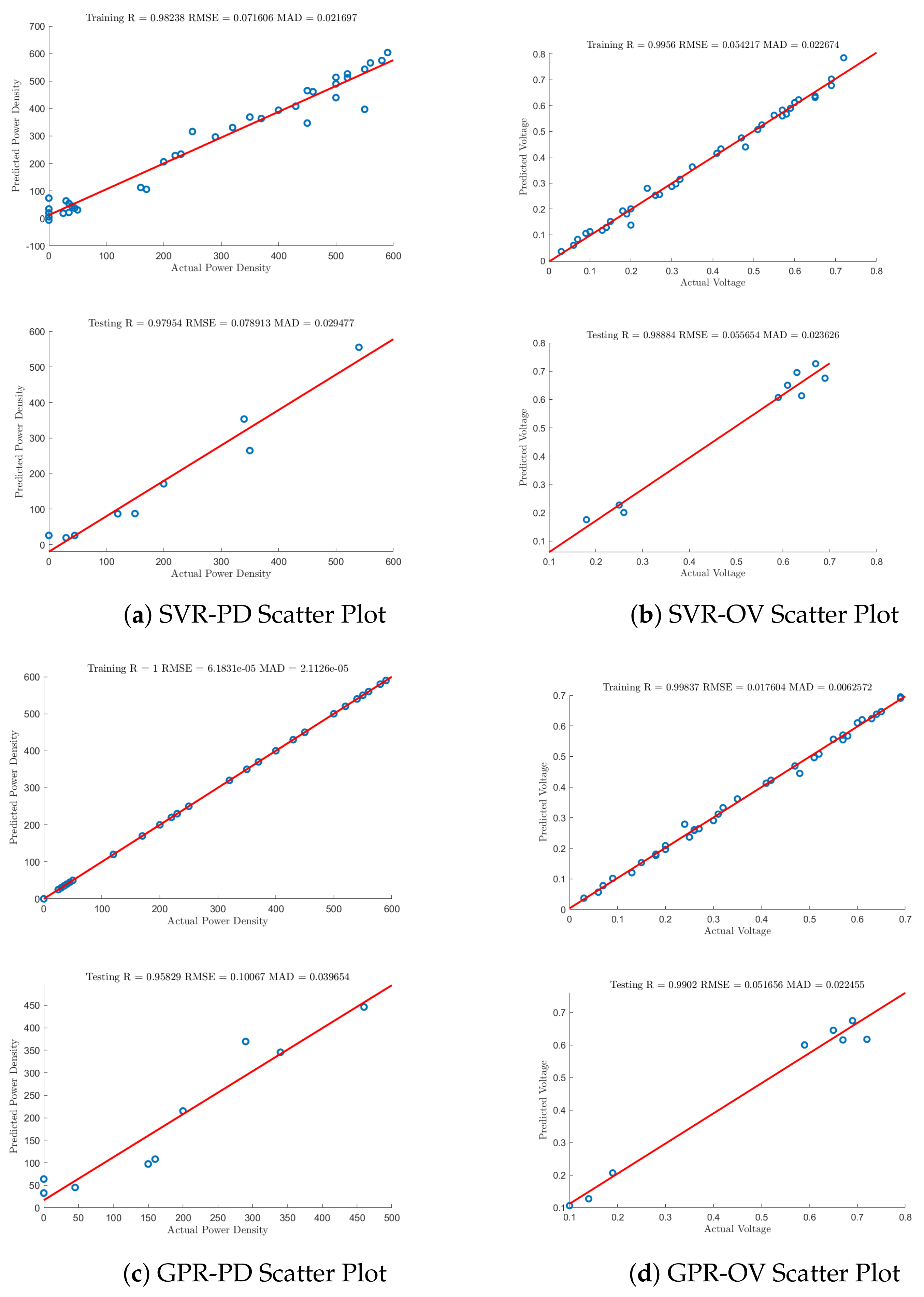
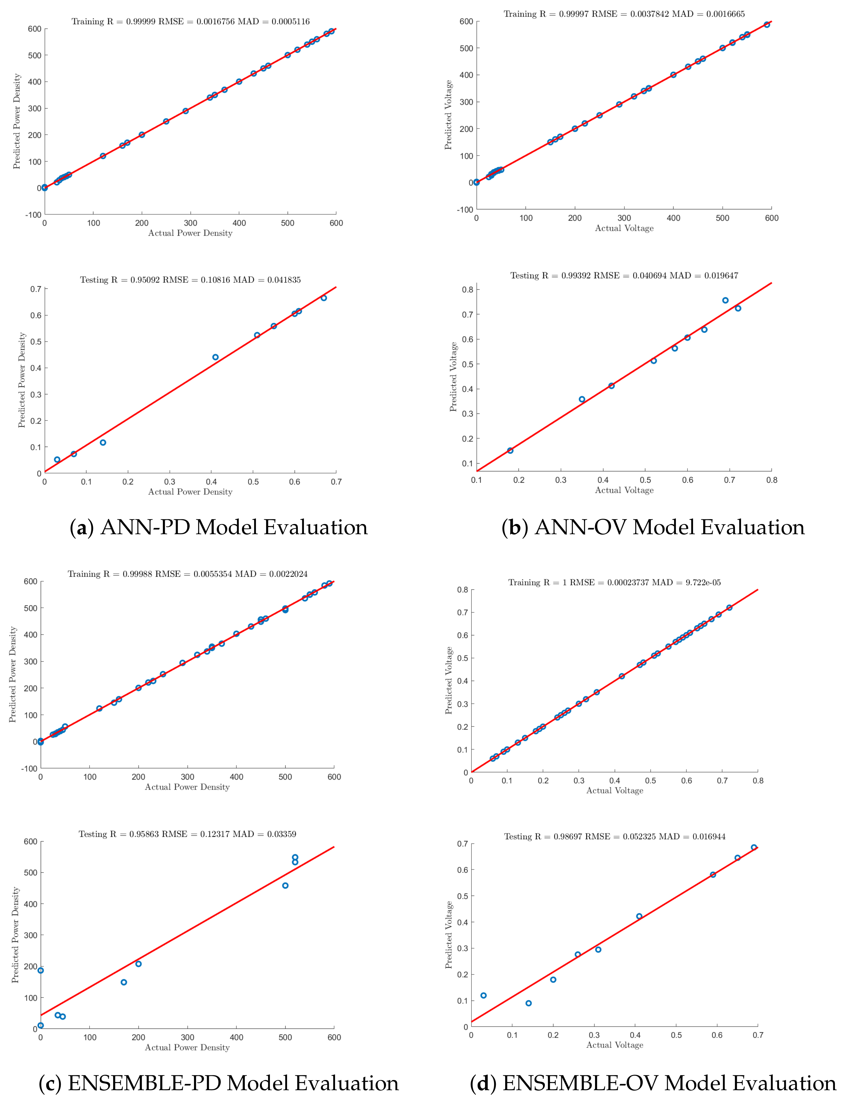
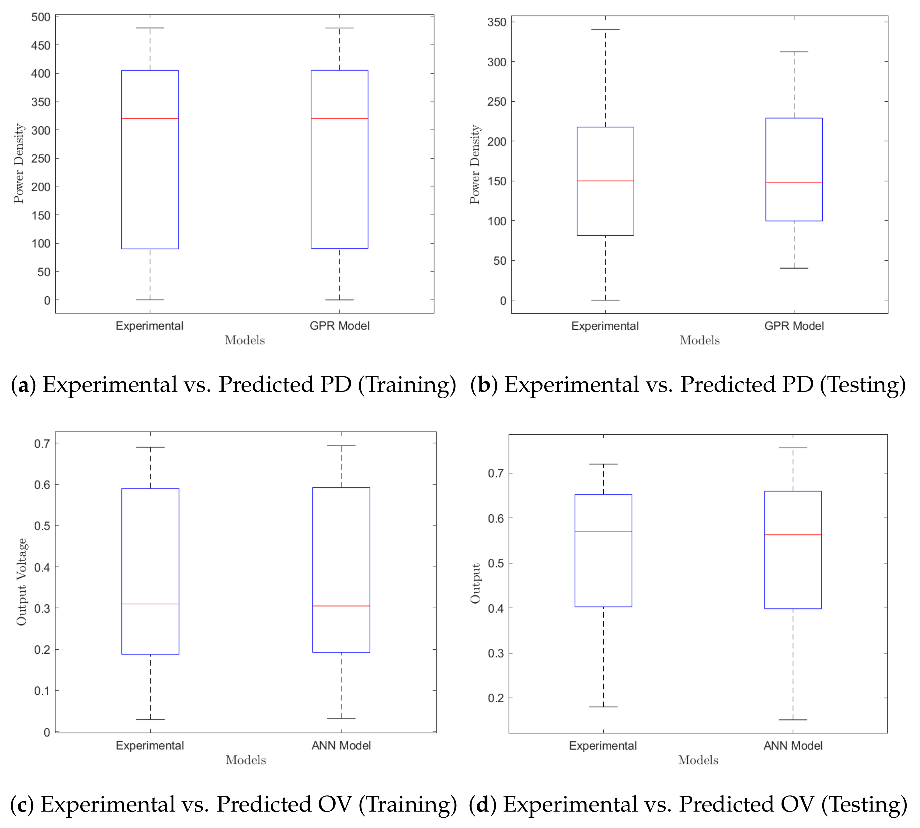
• The performances of four different machine learning algorithms, namely support vector regression, Gaussian process regression, artificial neural networks, and ensemble learners, are evaluated in modeling a microbial fuel cell process.
• Two main model structures are investigated for evaluating the optimal performance of the microbial fuel cell. In the first model structure, current density and anolyte concentration were considered as model inputs, while current density and chemical oxygen demand were considered as model inputs in the second model structure.
• The performance of each ML algorithm was optimized with grid search, Bayesian optimization, and random search to determine the model parameters that yield the optimal results.

The proposed models in this study may prove very useful for the design of efficient data-driven controllers for the MFC system or in the performance optimization of the MFC process. The remainder of the paper is organized as follows. Section 2 briefly discusses the experimental process from which the data used in this study are produced. In Section 3, we describe the methodology based on the three machine learning algorithms proposed in this study. Section 4 presents the results and discussions of the training and validation of the algorithm, and Section 5 provides some recommendations for future work.

2. Data

The experimental data used in this study were based on the synthesis of a microbial fuel cell (shown in Figure 2) conducted in [32], where the effects of acetate concentration and flow rate on microbial fuel cell performance were investigated. The microbial fuel cell fabricated in [32] was based on graphite electrodes, and the chemical compositions of the microbial cell culture are given in

Table 1. Chemical compositions in the fuel cell chamber.

Chemical Formula and Quantity
NaCl	0.5 g/L
CH3COONa·3H2O	1.13 g/L
NH4Cl	0.1 g/L
MgSO4·7H2O	0.1 g/L
NH2HPO4·12H20	15.3 g/L
KH2PO4	3 g/L
CaCl2	11 mg/L
Trace Elements	1.0 mL/L

. The fuel cell structure features a Y-shaped channel fabricated from two polymethylmethacrylate and two graphite plates. According to [32], the fuel cell produces a peak power of $618\pm 4$ mWh⁻¹, with a chemical oxygen demand (COD) of 1500 mg/L and an anolyte flow rate of 10 mL/h. During the inoculation process and prior to any experiments, pure nitrogen and argon were purged into the culture medium for 15 min to displace any dissolved oxygen. The individual electrode potentials of the anode and cathode were obtained using a Ag/AgCl reference electrode at the outlet of the microchannel.

An Agilent 39740 was used to collect data such as the anode and cathode potentials and cell voltages of the fuel cell every 15 s. Polarization curves of the MFC were obtained by varying the external resistance of the cell between $0.2$ and $10\times {10}^5\Omega$. For every change in external resistance, the MFC was observed until the cell voltage reached a steady state. Both the current and power densities were normalized to an anode area of 0.4 cm². All experiments were conducted in a temperature-controlled room of $25degC$, and the experiments were repeated three times to ensure that the data could be reproduced under similar conditions. We refer the reader to [32] for a more detailed explanation of this experimental procedure.

3. Methodology

3.1. Model Structures

Four machine learning-based algorithms, namely support vector regression (SVR), artificial neural networks (ANNs), Gaussian process regression (GPR), and Ensemble Learners are considered in this study to model the microbial fuel cell based on the experimental data in [32]. Two different datasets were considered in this study based on the experiments of [32]. The first experimental dataset was generated by studying the effect of anolyte concentration on microbial cell performance. The current densities and anolyte concentrations, which were considered as input features, were recorded against the power density and output voltages. The second experiment investigated the effect of chemical oxygen demand on cell performance. Based on these datasets, different ML-based models were developed for this microbial fuel cell. The first model set, termed Model-I, predicts power density (PD) and output voltage (OV) using anolyte concentration (AC) and current density (CD) as features. The second model set, termed Model-II, predicts power density and output voltage from current density (CD) and chemical oxygen demand concentration (CODC).

3.2. Modeling Algorithms

3.2.1. Artificial Neural Networks

Neural networks are artificial bio-inspired information-processing units that are capable of modelling nonlinear processes. Originally proposed by McCulloch and Pitts in 1943 in their attempt to model biosystems using a combination of simple logical operations, neural networks have evolved over the years, with more applications now being reported for deep neural networks and deep learning in science and engineering. The basic information processing unit in a neural network is mathematically represented by (1)

$$\begin{array}{ccc}\hfill \widehat{\mathcal{L}}& =& f\left(\sum _{i=1}^p{\omega }_i{x}_i+b\right),\hfill \end{array}$$

(1)

where $\omega$ and b denote synaptic weights and biases, respectively.

As with many other machine learning algorithms, the goal of a neural network for function-fitting applications is to model a physical process described by some data by finding an unbiased function approximation obtained based on the training dataset of the physical process. Neural network applications have also been developed to model fuel cell processes. Artificial neural networks were used to predict electricity production in a membrane-less microbial fuel cell [33], where glucose was considered as the primary electron donor. The effect of anode inclination on the power output of a mediator-less microbial fuel cell was studied in [34] using artificial neural networks, where it was discovered that lower COD removal and power generation occurred when the anodes were positioned at $0deg$ and $45deg$. A feedforward backpropagation neural network was utilized in [35] to simulate the polarization effects of cylindrical MFCs with different separation medium materials. In [36], an ANN was employed in conjunction with a microbial fuel cell as a biosensor to detect three organic pollutants: aldicarb, dimethyl-methylphosphonate (DMMP), and bisphenol-A (BPA).

In the present study, we employed a feedforward fully connected artificial neural network with a ReLU activation function to train models for predicting the output voltage and power density from two different pairs of inputs, current density and anolyte concentration in the first set and current density and COD concentration in the second set. In total, the first dataset consisted of 45 points and the second dataset consisted of 46 points. An 80:20 split between the training and testing sets was considered for all developed models.

3.2.2. Support Vector Regression

The support vector regression (SVR) proposed by [37] is based on structural risk minimization where, given a labeled training data set $\mathrm{\Pi }={\left\{(x_i,y_i)\right\}}_i^n$, the goal is to find a function $\mathcal{F}\left(x\right)$ (2) such that (3) is minimized.

$$\begin{array}{c}\hfill \mathcal{F}\left(x\right)=\omega \varphi \left(x\right)+\beta ,\end{array}$$

(2)

$$\begin{array}{c}\hfill \sum _{i=1}^n(y_i-f\left(x_i\right))<ϵ,\end{array}$$

(3)

$x_i\in {\mathbb{R}}^m$ and $y_i\in \mathbb{R}$ represent features and target, respectively. In (2), $\omega$ and $\beta$ represent weights and bias to be determined, while $\varphi (.)$ represents a nonlinear feature map in some predefined kernel feature space. The objective (3) is realized through the minimization of the function (4)

$$\begin{array}{c}\hfill R\left(f\right)=C{\displaystyle \frac{1}{n}}\sum _{i-1}^n{\mathcal{L}}_{ϵ}(\mathcal{F}\left(x_i\right)-y_i)+{\displaystyle \frac{1}{2}}{\left|\omega \right|}^2,\end{array}$$

(4)

The term ${\displaystyle \frac{1}{2}}{\left|\omega \right|}^2$ reduces the risk of overfitting through the estimation of the differential flatness of the function space. Different forms of loss function $\mathcal{L}$ can be defined for this problem. A popular loss function takes the form of (5)

$$\mathcal{L}=\left\{\begin{array}{ll}\left|f\right(x)-y|-ϵ& \left|\mathcal{F}\right(x)-y|\ge ϵ\\ 0& \mathrm{otherwise}.\end{array}\right.$$

(5)

In (4), the parameter C penalizes deviations of each sample from the specified error bound. Different forms of kernel functions have been proposed for the SVR algorithm. Popular kernel functions include polynomial, linear, radial basis, exponential radial basis, spline, and b-spline. The success of the SVR algorithm on a given modeling problem relies on the proper selection of its hyperparameters.

Over the past few decades, researchers in the physical and social sciences have pivoted the use of machine learning to build artificial systems from data that can offer an accurate representation of the real processes under consideration. Support vector machine and regression have received considerable attention. Some contributions to the application of support vector regression in chemical processes include [38,39,40,41]. Some results have also been reported for support vector regression in modelling microbial fuel cell processes. In [42], the authors studied the space design method-based support vector regression modelling of $MFC-A^2/O$ equipment, where both the forward and inverse SVR models were investigated using a quadratic kernel function. The authors in [43] combined support vector regression and a crow search algorithm for modelling and optimization of a microbial fuel cell process based on microalgal wastewater treatment.

3.2.3. Gaussian Process Regression

Gaussian process regression is a statistical machine learning algorithm based on the principle of Gaussian processes. It has been applied to several regression problems in science and engineering to develop models capable of describing the complex relationship between a set of input features and process outputs. Consider a function $f\left(x\right)$ that describes a physical process modelled by a Gaussian process, where $x\in {\mathbb{R}}^{m\times n}$ represents the features of the process, n is the number of features, and m is the number of observations recorded from the physical process. The Gaussian process is characterized by the mean function $m\left(x\right)$ and covariance function $cov(x_i,x_j)$, where it is assumed that the sample space for each feature $x^j\in {\mathbb{R}}^{m\times 1}j=1,\dots n$ has a multivariate normal density, that is,

$$\begin{array}{c}\hfill f\left(x\right)\approx \mathcal{N}\left(m\right(x),K(x,x\left)\right),\end{array}$$

(6)

where $K(x_i,x_j)$ is a kernel function. For example, consider a squared exponential function of the form

$$\begin{array}{c}\hfill K(x_i,x_j)=s^{2}exp\left(-{\displaystyle \frac{|x_i-x_j{|}^2}{2{\ell }^2}}\right),\end{array}$$

(7)

where $s^2$ and ${\ell }^2$ denote the magnitude and length-scale hyperparameters that control the behavior of the kernel (covariance) function. Suppose that the probability density function describing the Gaussian process is given by (8)

$$\begin{array}{c}\hfill p(u,x)={\left(2\pi \right)}^{-0.5N}{\left|K\right|}^{-0.5}exp\left(-0.5u^T{K}^{-1}(x,x)u\right).\end{array}$$

(8)

The likelihood function (9) can be used to describe the data under the assumption that the observation points are affected independently and identically by Gaussian noise with variance ${\sigma }^2$:

$$\begin{array}{c}\hfill p\left(y\right|u,x)=\prod _{i=1}^N{\displaystyle \frac{1}{\sqrt{2\pi {\sigma }^2}}}exp\left(-{\displaystyle \frac{(y_i-f{\left(x_i\right)}^2)}{2{\sigma }^2}}\right).\end{array}$$

(9)

The posterior distribution of function f is computed via Baye’s rule as

$$\begin{array}{c}\hfill p\left(y\right|u\left|x\right)={\displaystyle \frac{p(y,u|x\left)p\right(u\left|x\right)}{p\left(y\right|x)}},\end{array}$$

(10)

and its log-marginal-likelihood function is given by (11)

$$\begin{array}{ccc}\hfill logp\left(y\right|x)& =\hfill & \int p\left(y\right|u,x\left)p\right(u\left|x\right)df\hfill \\ \hfill & =\hfill & -0.5y^T{(K(x,x)+{\sigma }^2{I}_N)}^{-1}y\hfill \\ \hfill & \hfill & -0.5log\left|K\right(x,x)\hfill \\ \hfill & \hfill & +{\sigma }^2{I}_N|-0.5Nlog2\pi .\hfill \end{array}$$

(11)

The prediction of y based on f from a new observation point $x^{*}$ is then given statistically as a function of the mean $\mathbb{E}\left[f^{*}\right]$ and variance $var\left[f^{*}\right]$ by (12) and (13):

$$\begin{array}{c}\hfill \mathbb{E}\left[f^{*}\right]=K(x^{*},x){(K(x,x)+{\sigma }^2{I}_N)}^{-1}\end{array}$$

(12)

$$\begin{array}{c}\hfill var\left[f^{*}\right]=K(x^{*},x^{*})-K(x^{*},x){(K(x,x)+{\sigma }^2{I}_N)}^{-1}K(x,x^{*}).\end{array}$$

(13)

Gaussian process regression was employed by [44] to model the relationship between the operating conditions and power outputs of a two-chamber microbial fuel cell process. The data for the MFC considered in this study were generated from experiments conducted on a two-chamber microbial fuel cell consisting of glucose and glutamic acid substrates.

3.2.4. Ensemble Learners

Ensemble algorithms refer generally to a class of machine learning algorithms that combine two or more techniques towards improving the performance of weak machine learning algorithms. Different ensemble learning frameworks have been proposed depending on the voting mechanism, such as voting-based ensemble [45], ensemble of online sequential extreme learning machine [46], and weighted voting ensemble [47]. In this study, we consider an ensemble learning algorithm consisting of bagged or boosted regression trees. Hyperparameters of the ensemble learners includes method, number of learning cycles, learning rate, minimum lead size, and number of variables to sample.

3.3. Hyperparameter Optimization

Three different hyperparameter optimization algorithms, namely Bayesian optimization, grid search, and random search, were used to optimize the structure of the machine learning models. The Bayesian optimization algorithm falls into a class of machine learning optimization algorithms that are primarily concerned with the problem (14)

$$\begin{array}{c}\hfill \underset{x\in A}{max}f\left(A\right)\end{array}$$

(14)

where the objective function and the feasible set are assumed to possess the following characteristics [48]:

• The structure of f is typically unknown and cannot be described with attributes such as concavity or linearity.
• The nature of the optimization problem is derivative-free; this means that only the evaluation of $f\left(x\right)$ is observed and not first or second derivatives, thus preventing the application of popular gradient descent methods.
• The size of input $x\in {\mathbb{R}}^m$ is typically not large, with $m\le 20$.
• f is computationally expensive to evaluate; therefore, the number of objective function evaluations to be performed is limited to a few hundred.
• The membership of the feasibility set is assessable due to the simplicity of A.

Grid search is a classical hyperparameter optimization method that involves making an exhaustive search over the possible hyperparameter space. This search algorithm employs a brute-force approach to finding the optimal set of hyperparameters for the machine learning algorithms. The grid search algorithm maps the hyperparameter space into a predefined grid size depending on the possible range of values for each hyperparameter. In instances where there are numerous hyperparameters to be optimized, grid search may not be very efficient, although it is a very reliable hyperparameter optimization scheme depending on the density of the grid.

Random search, as the name implies, searches randomly in the hyperparameter space for the optimal set that yields the best performance. It is preferable in optimization problems where derivatives of the cost function may not exist. The random search begins with an initial guess sampled with the hyperparameter space and this guess is updated randomly over a given number of iterations until a termination criterion is satisfied. Different variants of the random search algorithm have been proposed in the literature. Some typical examples include the Friedman–Savage procedure, Fixed Step Size Random Search (FSSRS), Adaptive Step Size Random Search (ASSRS), and Optimized Relative Step Size Random Search (ORSSRS). These algorithms differ in the method of sampling of the search space.

4. Results and Discussion

The results obtained from the machine learning models used in this study are presented in this section. Two different model formulations are considered for power density and output voltage. The first model considers current density (CD) and anolyte concentration (AC) as input features, while the second model considers current density (CD) and chemical oxygen demand concentration (CODC) as input features. For the purposes of the discussions in this section, the first model is denoted as Model I, while the second model formulation is denoted as Model II. The abbreviations PD-I and OV-I refer to power density and output voltage models derived from CD and AC, while PD-II and OV-II connote power density and output voltage modeling from CD and CODC. First, we present the results obtained from hyperparameter tuning of each of these models for all the algorithms, then we discuss comparatively each of the selected best machine learning algorithms for all the process variables modeled. The performance of the models is compared using the correlation coefficient (R), mean squared error (MSE), and mean absolute deviation (MAD), defined by Equations (15)–(17), respectively.

$$\begin{array}{ccc}\hfill MSE& =& {\displaystyle \frac{1}{n}}\sum _{i=1}^n{(y_i-{\widehat{y}}_i)}^2\hfill \end{array}$$

(15)

$$\begin{array}{ccc}\hfill MAD& =& {\displaystyle \frac{1}{n}}\sum _{i=1}^n|y_i-{\widehat{y}}_i|\hfill \end{array}$$

(16)

$$\begin{array}{ccc}\hfill R& =& {\displaystyle \frac{{\sum }_m{\sum }_n(A_{mn}-\overline{A})(B_{mn}-\overline{B})}{\sqrt{\left({\sum }_m{\sum }_n{(A_{mn}-\overline{A})}^2\right)\left({\sum }_m{\sum }_n{(B_{mn}-\overline{B})}^2\right)}}}\hfill \end{array}$$

(17)

4.1. Hyperparameter Optimization

In this section, we provide some discussions on the results of the hyperparameter optimizations of the machine learning algorithms used in our study. The performance of the tuning algorithms was compared using the objective loss function $H_{obj}$ (18), which depends on the computed mean squared error (mse). A total of 100 iterations were considered for each of the optimization methods.

$$\begin{array}{c}\hfill H_{obj}=log(1+mse)\end{array}$$

(18)

4.1.1. Support Vector Regression

Table 2. SVR hyperparameter optimization results.

Model	BC	KS	Epsilon	KF	PO	Standardize	MO
Bayesian Optimization
PD-I	97.01	-	15.83	polynomial	4	true	8.22
OV-I	0.64	-	0.000804	polynomial	4	true	0.0082
PD-II	432.28	-	8.49	polynomial	3	true	7.71
OV-II	245.92	-	0.013731	polynomial	4	true	0.0026
Grid Search
PD-I	215.44	-	0.23351	polynomial	4	true	8.4966
OV-I	2.1544	-	0.00021497	polynomial	2	true	0.0088
PD-II	215.44	-	15.01	polynomial	4	true	7.8279
OV-II	0.46416	-	0.047607	polynomial	3	true	0.0057
Random Search
PD-I	210.61	-	69.337	polynomial	2	true	8.3156
OV-I	314.43	2.2181	0.018786	gaussian	-	true	0.0067
PD-II	79.263	-	29.712	polynomial	3	true	7.9745
OV-II	1.7538	-	0.00074444	polynomial	4	true	0.0030

presents the hyperparameter tuning results using Bayesian optimization, grid search, and random search for the SVR algorithm. Based on the obtained results, Bayesian optimization produced the best hyperparameters for PD-I, PD-II, and OV-II, while in the case of OV-I, the best hyperparameters were obtained with random search. The optimization process for the SVR algorithm reveals that PD-I and PD-II are modeled with a polynomial kernel function of order 4 and 3, respectively. OV-I is modeled with a Gaussian kernel with a kernel scale of 2.2, while OV-II is modeled with a polynomial kernel of order 4.

4.1.2. Gaussian Process Regression

Table 3. GPR hyperparameter optimization results.

Model	Sigma	Basis Function	Kernel Function	Kernel Scale	Standardize	MO
Bayesian Optimization
PD-I	0.12	pureQuadratic	ardmatern32	-	true	8.11
OV-I	0.0035	linear	ardexponential	-	false	0.0026
PD-II	0.013542	pureQuadratic	ardmatern32	-	false	7.9363
OV-II	0.00010833	pureQuadratic	matern52	1916.4	false	0.0012
Grid Search
PD-I	1.0276	constant	matern32	10.444	true	8.0036
OV-I	0.07247	none	matern32	2.25	true	0.0050103
PD-II	0.18217	none	exponential	928.32	false	7.7791
OV-II	0.024824	pureQuadratic	ardsquaredexponential	-	true	0.00056799
Random Search
PD-I	0.00028081	none	ardmatern52	-	true	7.6804
OV-I	0.00062233	linear	ardmatern32	-	true	0.0027988
PD-II	13.057	none	ardrationalquadratic	-	true	7.9585
OV-II	0.020	linear	ardmatern52	-	true	0.00070001

summarizes the results of the hyperparameter tuning for the GPR algorithm. The results reveal that the best hyperparameters for PD-I and PD-II are obtainable with the random and grid search algorithms, respectively, while the best hyperparameters for OV-I and OV-II were obtained with Bayesian and grid search algorithms, respectively. PD-I and PD-II were modeled with ardmatern52 and exponential kernel functions. In both models, no basis functions were utilized. OV-I and OV-II were modeled with ardexponential and ardsquaredexponential kernel functions, respectively. The basis function utilized for OV-I was a linear basis function, while OV-II required no basis functions.

4.1.3. Artificial Neural Networks

The hyperparameter optimization results for the ANN algorithm are summarized in

Table 4. ANN hyperparameter optimization results.

Model	Activations	Lambda	LWI	LBI	LayerSize	Standardize	MO
Bayesian Optimization
PD-I	tanh	0.545	he	zeros	[87 255 127]	true	7.85
OV-I	sigmoid	$2.9\times {10}^{-7}$	he	ones	[287 119]	true	0.0024
PD-II	relu	$3.41\times {10}^{-7}$	he	zeros	[214 241]	true	7.04
OV-II	relu	$2.72\times {10}^{-7}$	he	zeros	[33]	true	0.0012
Grid Search
PD-I	tanh	0.099828	glorot	ones	[13]	true	8.1602
OV-I	sigmoid	$2.78\times {10}^{-7}$	glorot	ones	[300 159 159]	true	0.0043
PD-II	relu	16.202	glorot	zeros	[24 159]	true	7.8778
OV-II	tanh	$4.5084\times {10}^{-7}$	he	ones	[4 2 7]	true	0.0013415
Random Search
PD-I	relu	$2.569\times {10}^{-5}$	he	ones	[5 190]	true	7.7136
OV-I	sigmoid	$2.1701\times {10}^{-5}$	glorot	ones	[89 2]	true	0.003678
PD-II	tanh	0.052638	he	ones	[52 155]	true	8.0649
OV-II	tanh	$1.4533\times {10}^{-6}$	he	ones	[5 11]	true	0.00056841

. In this instance, the best hyperparameters for PD-I and PD-II were obtained via random search and Bayesian optimization, respectively, while the optimal results obtained for OV-I and OV-II were derived from Bayesian and random search, respectively. PD-I and PD-II both have two hidden layers and employ a relu activation function; however, PD-I uses 5 and 190 neurons in layers 1 and 2, respectively, while PD-II uses 214 and 241 neurons in layers 1 and 2, respectively. OV-I and OV-II both have two hidden layers. There are 287 and 119 neurons in the hidden layers of OV-I, while OV-II has 5 and 11 neurons in its hidden layers. OV-I and OV-II employ sigmoid and tanh activation functions.

4.1.4. Ensemble Learning

In

Table 5. Ensemble hyperparameter optimization results.

Model	Method	NLC	LR	MLS	MNS	VS	MO
Bayesian Optimization
PD-I	LSBoost	288	0.14	1	34	1	8.14
OV-I	LSBoost	432	0.89	3	2	2	0.019
PD-II	LSBoost	16	0.4303	1	36	1	8.2865
OV-II	LSBoost	155	0.0827	4	2	1	0.0021
Grid Search
PD-I	LSBoost	324	0.046416	2	11	2	8.6515
OV-I	LSBoost	324	0.46416	4	7	2	0.0033
PD-II	LSBoost	37	0.46416	1	36	2	7.7934
OV-II	LSBoost	324	0.21544	1	24	2	0.0014
Random Search
PD-I	LSBoost	389	0.21924	3	8	1	8.2468
OV-I	LSBoost	251	0.14145	2	9	1	0.0044
PD-II	LSBoost	317	0.042925	1	10	1	7.9872
OV-II	LSBoost	65	0.39092	1	35	2	0.0016

, we summarize the results of the hyperparameter optimization. The best results for PD-I and PD-II were obtained from Bayesian and grid search optimization, respectively, while the optimal results for OV-I and OV-II were derived from grid search. The ensemble algorithm employed the LSBoost method in all the instances for fitting the regression trees. In the case of PD-I, the ensemble algorithm samples only one variable over 288 learning cycles, while with PD-II, the algorithm samples all two input variables over just 37 cycles. The ensemble algorithms for OV-I and OV-II samples both input features over 324 learning cycles in both instances.

4.2. Model Comparisons

In

Table 6. Model I—performance measures.

	Training			Testing
Model	$\mathbf{R}$	RMSE	MAD	$\mathbf{R}$	RMSE	MAD
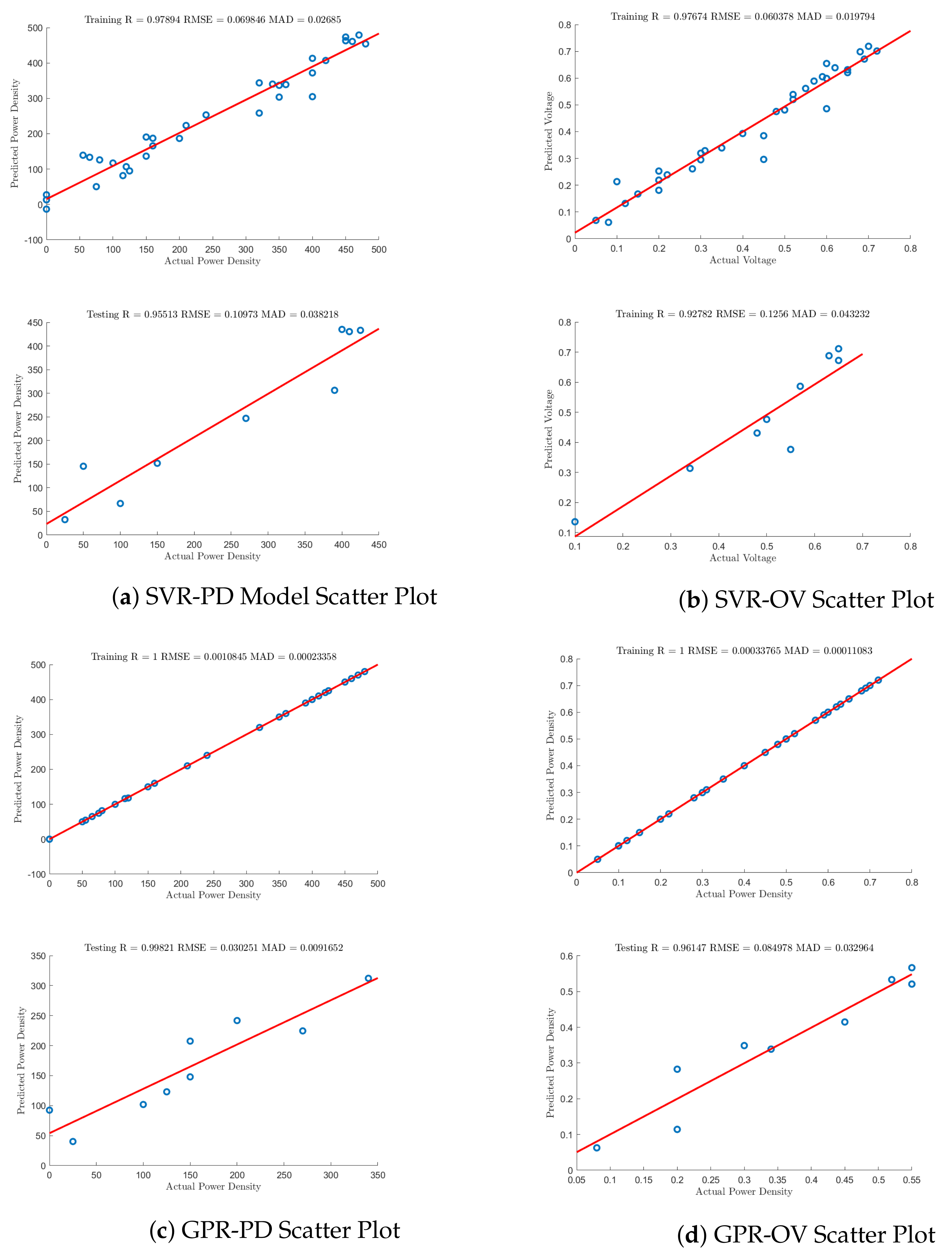
PD-SVR	0.9789	0.0698	0.0268	0.9153	0.1097	0.0382
PD-GPR	1.0000	0.0010	0.0002	0.9982	0.0302	0.0091
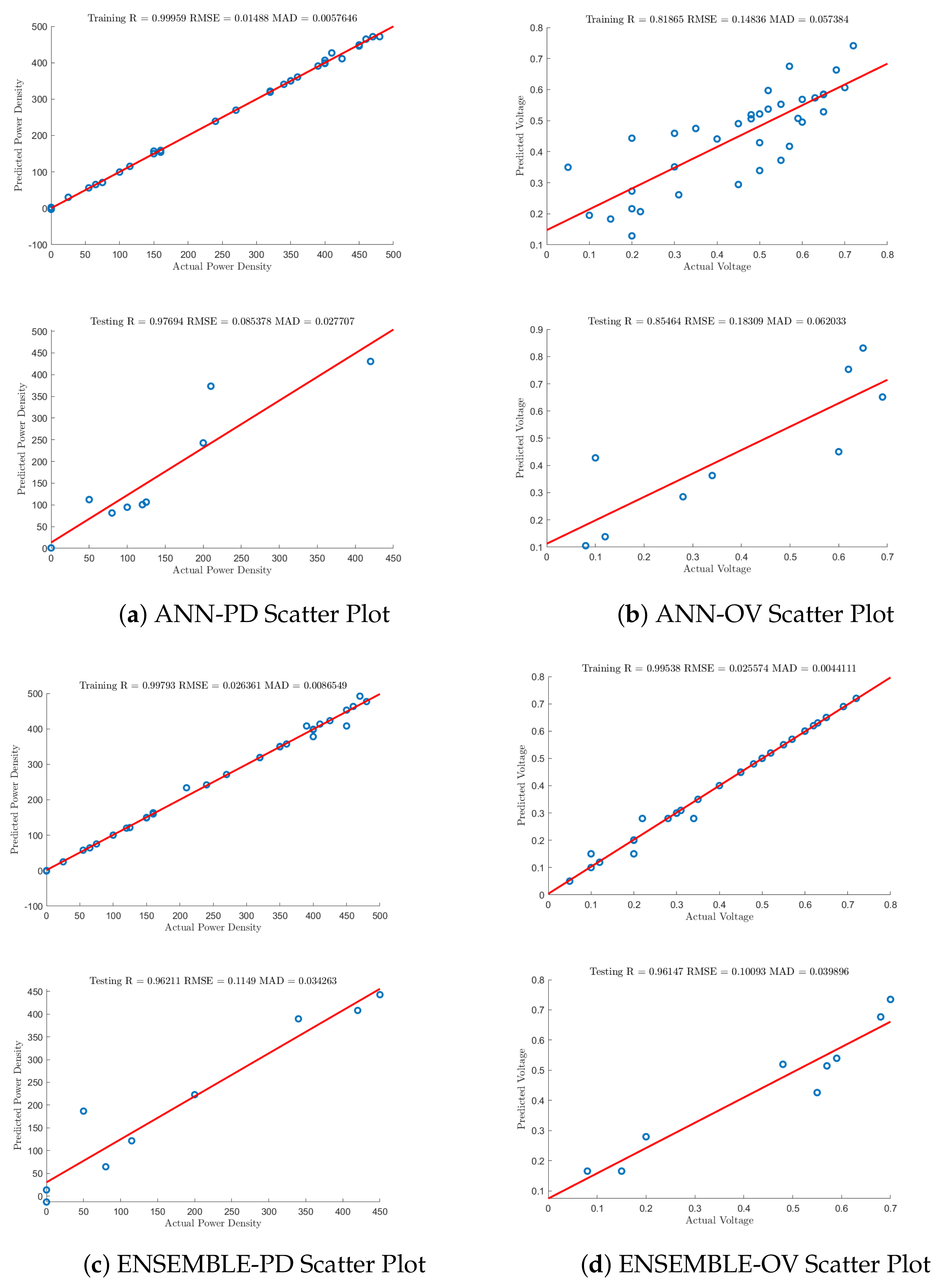
PD-ANN	0.9995	0.0148	0.0057	0.9769	0.0854	0.0277
PD-ENSEMBLE	0.9973	0.0263	0.0086	0.9621	0.1149	0.0342
OV-SVR	0.9767	0.0600	0.0197	0.9278	0.1256	0.0432
OV-GPR	1.0000	0.0003	0.0001	0.9614	0.0850	0.0330
OV-ANN	0.8186	0.1483	0.0057	0.8546	0.1831	0.0620
OV-ENSEMBLE	0.9953	0.0255	0.0044	0.9614	0.1009	0.0399

, we summarize and compare the performances of the modeling algorithms for Model I. Figure 3 and Figure 4 present the regression plots for each of the machine learning algorithms based on Model-I structure. The analyses here are based on the selected best models from the hyperparameter tuning process. The evaluations of these models are discussed based on the R, RMSE, and MAD values defined in (15)–(17). The best performance based on the testing evaluation results for PD prediction with Model I formulation is the GPR algorithm with performance values of (1.0000, 0.0010, 0.0002) and (0.9982, 0.0302, 0.0091) on the training and testing sets, respectively. Next is the ANN algorithm, with training and testing performance values of (0.9995, 0.0148, 0.0057) and (0.9769, 0.0854, 0.0277), respectively. The ENSEMBLE algorithm follows, with training and testing performance values of (0.9973, 0.0263, 0.0086) and (0.9621, 0.1149, 0.0342), while the SVR comes last, with performance values of (0.9789, 0.0698, 0.0268) and (0.9153, 0.1097, 0.0382) on training and testing sets, respectively.

The best algorithm for the prediction of output voltage using Model I structure was obtained with the GPR algorithm with training and testing performance values of (1, 0.0003, 0.0001) and (0.9614, 0.0850, 0.0330), respectively. Next comes the ENSEMBLE algorithm, with performance values of (0.9953, 0.0255, 0.0044) and (0.9614, 0.1009, 0.0399) on training and testing sets, respectively. The SVR algorithm follows, with (0.9767, 0.06,0.0197) and (0.9278, 0.1256, 0.0432) on training and testing evaluations, while the ANN algorithm comes last, with (0.8186, 0.1483, 0.0057) and (0.8546, 0.1831, 0.0620) on training and testing evaluations, respectively.

Table 7. Model II—performance measures.

	Training			Testing
Model	$\mathbf{R}$	RMSE	MAD	$\mathbf{R}$	RMSE	MAD
PD-SVR	0.9824	0.0716	0.0217	0.9795	0.0789	0.0295
PD-GPR	1.0000	0.00006	0.00002	0.9583	0.1006	0.0039
PD-ANN	0.9995	0.01488	0.0057	0.9769	0.0854	0.0277
PD-ENSEMBLE	0.9979	0.0263	0.0086	0.9621	0.1149	0.0342
OV-SVR	0.9956	0.0542	0.0223	0.9888	0.0556	0.0236
OV-GPR	0.9983	0.0176	0.0062	0.9902	0.0516	0.0224
OV-ANN	0.9999	0.0003	0.0016	0.9939	0.0406	0.0196
OV-ENSEMBLE	1.0000	0.0002	0.00009	0.9869	0.0523	0.01694

summarizes and compares the algorithms for Model-II-based representation of the prediction problem. Figure 5 and Figure 6 present the regression plots for each of the machine learning algorithms based on the Model-I structure. Based on the testing evaluation results, it can be concluded that the SVR algorithm performed best for modeling power density, with performance values of (0.9824, 0.0716, 0.0217) and (0.9795, 0.0789, 0.0295) on training and testing set evaluations, respectively. Next is the ANN algorithm, with performance values of (0.9995, 0.0148, 0.0057) and (0.9769, 0.0854, 0.0277) on training and testing evaluations. The ENSEMBLE algorithm follows, with values of (0.9979, 0.0263, 0.0086) and (0.9621, 0.1149, 0.0342) on training and testing predictions. Finally, the GPR algorithm comes last, with training and testing evaluation values of (1, 0.00006, 0.00002) and (0.9583, 0.1006, 0.0039), respectively. The best algorithm for predicting output voltage using Model-II formulation is the ANN algorithm, with performance evaluations of (0.9999, 0.0003, 0.0016) and (0.9939, 0.0406, 0.0196) on the training and testing sets, respectively. The GPR algorithm follows, with training and testing evaluations of (0.9983, 0.0176, 0.0062) and (0.9902, 0.0516, 0.0224), respectively. Next is the SVR algorithm, with (0.9956, 0.0542, 0.0223) and (0.9888, 0.0556, 0.0236) on training and testing evaluations, while the ENSEMBLE algorithm comes last, with performance values of (1, 0.0002, 0.00009) and (0.9869, 0.0523, 0.01694) on training and testing evaluations. Based on the analyses carried out, it can be summarized that Model I is more suitable for modeling power density, while Model II formulation models the output voltage of the MFC better.

Table 8. Model I—Power density predictions.

Current Density	Anolyte Concentration	Power Density (Exp)	Power Density (Pred)
Training
0	5	0	0.34339813
100	5	75	74.2800234
150	5	100	99.88043377
300	5	120	117.9662687
400	5	80	81.67882275
450	5	65	64.99960065
750	5	50	50.02761297
0	10	0	−0.041741094
500	10	320	319.9249303
750	10	400	399.9600416
1000	10	350	350.0020362
0	20	0	0.027481016
500	20	360	359.9074023
750	20	410	410.1444232
1250	20	400	400.0602652
1500	20	320	319.9797993
0	40	0	−0.005480526
250	40	160	160.0652346
500	40	350	349.9075691
1000	40	450	450.0548606
1250	40	480	479.9573814
1750	40	210	210.0434299
250	60	150	149.9998696
1000	60	400	400.0033257
1500	60	470	470.0090551
1750	60	450	449.9858254
2250	60	390	389.980239
200	5	115	116.3443356
750	40	425	425.0127718
1250	60	460	459.9801203
1000	20	450	449.8780158
250	10	160	160.113909
500	5	55	54.51161768
1500	40	400	399.9589216
2000	60	420	420.0173303
1250	10	240	240.0113957
Testing
50	5	25	40.19067673
250	5	125	123.0486118
1500	10	150	147.878756
1750	20	200	241.7814819
0	60	0	92.46039675
500	60	270	224.54181
750	60	340	312.1917304
350	5	100	101.8892903
250	20	150	207.4972159

and

Table 9. Model II—output voltage predictions.

Current Density	Chemical Oxygen Demand	Voltage (Exp)	Voltage (Pred)
Training
0	100	0.3	0.301292574
50	100	0.27	0.270779805
100	100	0.25	0.240441584
200	100	0.18	0.181072746
250	100	0.15	0.152516957
300	100	0.14	0.12507906
400	100	0.07	0.074770924
450	100	0.06	0.052516078
500	100	0.03	0.032575835
250	500	0.67	0.668121708
750	500	0.61	0.607594451
1000	500	0.58	0.578752368
1500	500	0.24	0.240130435
1750	500	0.13	0.129828615
250	1000	0.65	0.651108508
500	1000	0.61	0.60898659
1750	1000	0.26	0.260703735
0	1500	0.69	0.69378588
250	1500	0.65	0.647309106
750	1500	0.57	0.566099365
1500	1500	0.32	0.323114972
1750	1500	0.26	0.256997405
2000	1500	0.2	0.200363296
0	2000	0.69	0.686585999
750	2000	0.55	0.554208041
1250	2000	0.41	0.409063645
1500	2000	0.31	0.305269093
1750	2000	0.19	0.196320251
2000	2000	0.1	0.096873135
150	100	0.2	0.210465426
350	100	0.09	0.099060228
500	500	0.63	0.633262151
1000	2000	0.51	0.508001665
750	1000	0.59	0.592736549
1250	1000	0.47	0.470245135
500	2000	0.59	0.592277611
1250	500	0.48	0.480093074
Testing
0	500	0.72	0.72386166
0	1000	0.69	0.756116272
1000	1000	0.57	0.562841991
1500	1000	0.35	0.357919862
2000	1000	0.18	0.151244441
500	1500	0.6	0.605950688
1000	1500	0.52	0.512822799
250	2000	0.64	0.638189001
1250	1500	0.42	0.411916742

summarize the model outputs on training and testing set evaluations with respect to the experimental outputs.

Figure 7 compares pictorially the experimental predictions from the data-driven models and expresses that the data-driven MFC model presented in this study agrees significantly with the experimental data. Authors in [2] examine by experimentation the effect of varying COD concentration and anolyte flow rate on the performance outputs of the MFC. According to their experimental data, the poorest performance was observed for the MFC at low influent COD concentrations of 100 mg L⁻¹ due to low fuel supply. The data-driven model similarly gives the same output demonstrating concrete agreement with the experimental values. Furthermore, it was proposed in [2] that variations in anolyte concentrations significantly affect the power density outputs of the MFC. Likewise, we find in our data-driven model development a strong agreement with this assertion, as the best model for predicting power density is the Model-I with anolyte concentration and current density as inputs. The proposed data-driven soft computing models proposed in this study can be used in a parallel configuration to predict power density and voltage outputs of a two-chamber MFC. The first block, which predicts power density, will feature the GPR optimized model, which takes anolyte concentrations and current density as input. The second block in the parallel configuration will feature the ANN optimized output voltage prediction model, taking as inputs CODC and current density.

5. Conclusions

In summary, we presented different machine learning-based models, namely support vector regression, Gaussian regression, artificial neural networks, and ensemble learning for predicting both output voltage and power density from experimental datasets with features including current density, anolyte concentration, and chemical oxygen demand. Three different hyperparameter optimization methods were employed to determine the best hyperparameters for each machine learning algorithm. In each modeling instance for power density and output voltage, one hyperparameter algorithm performed better than the other. Based on these results, we arrived at optimal models for Model-I and Model-II formulations for predicting power density and output voltage. The optimal models for the different machine learning algorithms were further compared towards proposing the best machine learning algorithm for the prediction of output voltage and power density. The best model for predicting power density was obtained from a GPR-algorithm-based model with 99% model accuracy and the best model for predicting output voltage is an ANN-based model with a 99% model accuracy. The proposed models in this study are particularly useful for design and soft computing applications for MFCs.

References

- Xia, C.; Zhang, D.; Pedrycz, W.; Zhu, Y.; Guo, Y. Models for Microbial Fuel Cells: A critical review. J. Power Sources 2018, 373, 119–131. [Google Scholar] [CrossRef]
- Garg, A.; Lam, J.S.L. Design of explicit models for estimating efficiency characteristics of microbial fuel cells. Energy 2017, 134, 136–156. [Google Scholar] [CrossRef]
- Mohamed, H.O.; Obaid, M.; Sayed, E.T.; Liu, Y.; Lee, J.; Park, M.; Barakat, N.A.M.; Kim, H.Y. Electricity generation from real industrial wastewater using a single-chamber air cathode microbial fuel cell with an activated carbon anode. Bioprocess Biosyst. Eng. 2017, 40, 1151–1161. [Google Scholar] [CrossRef]
- Min, B.; Logan, B.E. Continuous Electricity Generation from Domestic Wastewater and Organic Substrates in a Flat Plate Microbial Fuel Cell. Environ. Sci. Technol. 2004, 38, 5809–5814. [Google Scholar] [CrossRef] [PubMed]
- Jiang, J.; Zhao, Q.; Wei, L.; Wang, K.; Lee, D.J. Degradation and characteristic changes of organic matter in sewage sludge using microbial fuel cell with ultrasound pretreatment. Bioresour. Technol. 2011, 102, 272–277. [Google Scholar] [CrossRef]
- Nimje, V.R.; Chen, C.Y.; Chen, H.R.; Chen, C.C.; Huang, Y.M.; Tseng, M.J.; Cheng, K.C.; Chang, Y.F. Comparative bioelectricity production from various wastewaters in microbial fuel cells using mixed cultures and a pure strain of Shewanella oneidensis. Bioresour. Technol. 2012, 104, 315–323. [Google Scholar] [CrossRef] [PubMed]
- Asefi, B.; Li, S.L.; Moreno, H.A.; Sanchez-Torres, V.; Hu, A.; Li, J.; Yu, C.P. Characterization of electricity production and microbial community of food waste-fed microbial fuel cells. Process Saf. Environ. Prot. 2019, 125, 83–91. [Google Scholar] [CrossRef]
- Kebaili, H.; Kameche, M.; Innocent, C.; Ziane, F.; Sabeur, S.; Sahraoui, T.; Ouis, M.; Zerrouki, A.; Charef, M. Treatment of fruit waste leachate using microbial fuel cell: Preservation of agricultural environment. Acta Ecol. Sin. 2021, 41, 97–105. [Google Scholar] [CrossRef]
- Fujimura, S.; Kamitori, K.; Kamei, I.; Nagamine, M.; Miyoshi, K.; Inoue, K. Performance of stacked microbial fuel cells with Barley–Shochu waste. J. Biosci. Bioeng. 2022, 133, 467–473. [Google Scholar] [CrossRef]
- Chaturvedi, A.; Chaturvedi, A.; Nagaiah, T.C.; Kundu, P.P. Synthesis of Co/Ni @ Al2O3-GO as novel oxygen reduction electrocatalyst for sustainable bioelectricity production in single-chambered microbial fuel cells. J. Environ. Chem. Eng. 2021, 9, 106054. [Google Scholar] [CrossRef]
- Qavami, A.; Ghasemi, S. Nickel-cobalt manganate supported on reduced graphene oxide/carbon nanotube for improving air cathode performance in single chamber microbial fuel cell. Mater. Sci. Eng. B 2022, 275, 115492. [Google Scholar] [CrossRef]
- Kumar, V.; Rudra, R.; Hait, S. Sulfonated polyvinylidene fluoride-crosslinked-aniline-2-sulfonic acid as ion exchange membrane in single-chambered microbial fuel cell. J. Environ. Chem. Eng. 2021, 9, 106467. [Google Scholar] [CrossRef]
- Wang, H.; Chen, P.; Zhang, S.; Jiang, J.; Hua, T.; Li, F. Degradation of pyrene using single-chamber air-cathode microbial fuel cells: Electrochemical parameters and bacterial community changes. Sci. Total Environ. 2022, 804, 150153. [Google Scholar] [CrossRef] [PubMed]
- Esfandyari, M.; Fanaei, M.A.; Gheshlaghi, R.; Mahdavi, M.A. Neural network and neuro-fuzzy modeling to investigate the power density and Columbic efficiency of microbial fuel cell. J. Taiwan Inst. Chem. Eng. 2016, 58, 84–91. [Google Scholar] [CrossRef]
- Esfandyari, M.; Fanaei, M.A.; Gheshlaghi, R.; Mahdavi, M.A. Dynamic modeling of a continuous two-chamber microbial fuel cell with pure culture of Shewanella. Int. J. Hydrogen Energy 2017, 42, 21198–21202. [Google Scholar] [CrossRef]
- Xiao, B.; Yang, F.; Liu, J. Evaluation of electricity production from alkaline pretreated sludge using two-chamber microbial fuel cell. J. Hazard. Mater. 2013, 254–255, 57–63. [Google Scholar] [CrossRef]
- Nien, P.C.; Lee, C.Y.; Ho, K.C.; Adav, S.S.; Liu, L.; Wang, A.; Ren, N.; Lee, D.J. Power overshoot in two-chambered microbial fuel cell (MFC). Bioresour. Technol. 2011, 102, 4742–4746. [Google Scholar] [CrossRef]
- Wei, L.; Yuan, Z.; Cui, M.; Han, H.; Shen, J. Study on electricity-generation characteristic of two-chambered microbial fuel cell in continuous flow mode. Int. J. Hydrogen Energy 2012, 37, 1067–1073. [Google Scholar] [CrossRef]
- Wang, H.; Long, X.; Zhang, J.; Cao, X.; Liu, S.; Li, X. Relationship between bioelectrochemical copper migration, reduction and electricity in a three-chamber microbial fuel cell. Chemosphere 2020, 241, 125097. [Google Scholar] [CrossRef]
- Wang, C.; Shen, J.; Chen, Q.; Ma, D.; Zhang, G.; Cui, C.; Xin, Y.; Zhao, Y.; Hu, C. The inhibiting effect of oxygen diffusion on the electricity generation of three-chamber microbial fuel cells. J. Power Sources 2020, 453, 227889. [Google Scholar] [CrossRef]
- Yang, Z.; Li, J.; Chen, F.; Xu, L.; Jin, Y.; Xu, S.; Wang, J.; Shen, X.; Zhang, L.; Song, Y. Bioelectrochemical process for simultaneous removal of copper, ammonium and organic matter using an algae-assisted triple-chamber microbial fuel cell. Sci. Total Environ. 2021, 798, 149327. [Google Scholar] [CrossRef] [PubMed]
- Zhang, S.; Bao, R.; Lu, J.; Sang, W. Simultaneous sulfide removal, nitrification, denitrification and electricity generation in three-chamber microbial fuel cells. Sep. Purif. Technol. 2018, 195, 314–321. [Google Scholar] [CrossRef]
- Greenman, J.; Mendis, A.; You, J.; Gajda, I.; Horsfield, I.; Ieropoulos, I. Microbial Fuel Cell Based Thermosensor for Robotic Applications. Front. Robot. AI 2021, 8, 558953. [Google Scholar] [CrossRef]
- Tsompanas, M.A.I.; Adamatzky, A.; Sirakoulis, G.C.; Greenman, J.; Ieropoulos, I. Towards implementation of cellular automata in Microbial Fuel Cells. PLoS ONE 2017, 12, e0177528. [Google Scholar] [CrossRef] [Green Version]
- Kumar, R.; Singh, L.; Zularisam, A.W.; Hai, F.I. Microbial fuel cell is emerging as a versatile technology: A review on its possible applications, challenges and strategies to improve the performances. Int. J. Energy Res. 2017, 42, 369–394. [Google Scholar] [CrossRef] [Green Version]
- Santoro, C.; Arbizzani, C.; Erable, B.; Ieropoulos, I. Microbial fuel cells: From fundamentals to applications. A review. J. Power Sources 2017, 356, 225–244. [Google Scholar] [CrossRef]
- Philamore, H.; Rossiter, J.; Ieropoulos, I. Sub-millilitre Microbial Fuel Cell Power for Soft Robots. In Biomimetic and Biohybrid Systems; Springer: Berlin/Heidelberg, Germany, 2013; pp. 424–426. [Google Scholar]
- Feng, Y.; Barr, W.; Harper, W. Neural network processing of microbial fuel cell signals for the identification of chemicals present in water. J. Environ. Manag. 2013, 120, 84–92. [Google Scholar] [CrossRef]
- de Ramón-Fernández, A.; Salar-García, M.; Ruiz-Fernández, D.; Greenman, J.; Ieropoulos, I. Modelling the energy harvesting from ceramic-based microbial fuel cells by using a fuzzy logic approach. Appl. Energy 2019, 251, 113321. [Google Scholar] [CrossRef]
- Ghasemi, M.; Nassef, A.M.; Al-Dhaifallah, M.; Rezk, H. Performance improvement of microbial fuel cell through artificial intelligence. Int. J. Energy Res. 2020, 45, 342–354. [Google Scholar] [CrossRef]
- de Ramón-Fernández, A.; Salar-García, M.; Fernández, D.R.; Greenman, J.; Ieropoulos, I. Evaluation of artificial neural network algorithms for predicting the effect of the urine flow rate on the power performance of microbial fuel cells. Energy 2020, 213, 118806. [Google Scholar] [CrossRef] [PubMed]
- Ye, D.; Yang, Y.; Li, J.; Zhu, X.; Liao, Q.; Deng, B.; Chen, R. Performance of a microfluidic microbial fuel cell based on graphite electrodes. Int. J. Hydrogen Energy 2013, 38, 15710–15715. [Google Scholar] [CrossRef]
- Tardast, A.; Rahimnejad, M.; Najafpour, G.; Ghoreyshi, A.; Premier, G.C.; Bakeri, G.; Oh, S.E. Use of artificial neural network for the prediction of bioelectricity production in a membrane less microbial fuel cell. Fuel 2014, 117, 697–703. [Google Scholar] [CrossRef]
- Jaeel, A.J.; Al-wared, A.I.; Ismail, Z.Z. Prediction of sustainable electricity generation in microbial fuel cell by neural network: Effect of anode angle with respect to flow direction. J. Electroanal. Chem. 2016, 767, 56–62. [Google Scholar] [CrossRef]
- Tsompanas, M.A.; You, J.; Wallis, L.; Greenman, J.; Ieropoulos, I. Artificial neural network simulating microbial fuel cells with different membrane materials and electrode configurations. J. Power Sources 2019, 436, 226832. [Google Scholar] [CrossRef]
- King, S.T.; Sylvander, M.; Kheperu, M.; Racz, L.; Harper, W.F., Jr. Detecting recalcitrant organic chemicals in water with microbial fuel cells and artificial neural networks. Sci. Total Environ. 2014, 497–498, 527–533. [Google Scholar] [CrossRef]
- Vapnik, V. The Nature of Statistical Learning Theory; Information Science and Statistics; Springer: New York, NY, USA, 2000. [Google Scholar]
- Sahaluddin, M.; Alade, I.O.; Oyedeji, M.O.; Aliyu, U.S. A machine learning-based model to estimate the density of nanofluids of nitrides in ethylene glycol. J. Appl. Phys. 2020, 127, 205105. [Google Scholar] [CrossRef]
- Alade, I.O.; Rahman, M.A.A.; Saleh, T.A. Predicting the specific heat capacity of alumina/ethylene glycol nanofluids using support vector regression model optimized with Bayesian algorithm. Sol. Energy 2019, 183, 74–82. [Google Scholar] [CrossRef]
- Alade, I.O.; Oyedeji, M.O.; Rahman, M.A.A.; Saleh, T.A. Predicting the density of carbon-based nanomaterials in diesel oil through computational intelligence methods. J. Therm. Anal. Calorim. 2022, 147, 8699–8707. [Google Scholar] [CrossRef]
- Olumegbon, I.A.; Alade, I.O.; Sahaluddin, M.; Oyedeji, M.O.; Sa’ad, A.U. Modelling the viscosity of carbon-based nanomaterials dispersed in diesel oil: A machine learning approach. J. Therm. Anal. Calorim. 2021, 145, 1769–1777. [Google Scholar] [CrossRef]
- Wang, J.; Wang, Q.; Zhou, J.; Wang, X.; Cheng, L. Operation space design of microbial fuel cells combined anaerobic–anoxic–oxic process based on support vector regression inverse model. Eng. Appl. Artif. Intell. 2018, 72, 340–349. [Google Scholar] [CrossRef]
- Hossain, S.Z.; Sultana, N.; Mohammed, M.E.; Razzak, S.A.; Hossain, M.M. Hybrid support vector regression and crow search algorithm for modeling and multiobjective optimization of microalgae-based wastewater treatment. J. Environ. Manag. 2022, 301, 113783. [Google Scholar] [CrossRef] [PubMed]
- He, Y.J.; Ma, Z.F. A Data-Driven Gaussian Process Regression Model for Two-Chamber Microbial Fuel Cells. Fuel Cells 2016, 16, 365–376. [Google Scholar] [CrossRef]
- Cao, J.; Lin, Z.; Huang, G.B.; Liu, N. Voting based extreme learning machine. Inf. Sci. 2012, 185, 66–77. [Google Scholar] [CrossRef]
- Lan, Y.; Soh, Y.C.; Huang, G.B. Ensemble of online sequential extreme learning machine. Neurocomputing 2009, 72, 3391–3395. [Google Scholar] [CrossRef]
- Cao, J.J.; Kwong, S.; Wang, R.; Li, K. A weighted voting method using minimum square error based on Extreme Learning Machine. In Proceedings of the 2012 International Conference on Machine Learning and Cybernetics, Xi’an, China, 15–17 July 2012; IEEE: Piscataway, NJ, USA, 2012. [Google Scholar] [CrossRef]
- Frazier, P.I. A Tutorial on Bayesian Optimization. arXiv 2018, arXiv:1807.02811. [Google Scholar] [CrossRef]